Abstract

We investigate the performance of a large class of cosmic microwave background experiments with respect to their ability to measure various cosmological parameters. We pay special attention to the measurement of the total cosmological density, $\Omega$. We consider interferometer experiments, all-sky single-dish experiments, and also single-dish experiments with a deep-patch technique. Power spectrum estimates for these experiments are studied, and their induced errors in cosmological parameter estimates evaluated. Given this motivation we find various promising corners in the experiment parameter space surveyed. Low noise all-sky satellite experiments are the expensive option, but they are best suited for dealing with large sets of cosmological parameters. At intermediate noises we find a useful corner in high-resolution deep patch single-dish experiments. Interferometers are limited by sample variance, but provide the best estimates based on the very small angular scales. For all these experiments we present conservative, but still promising estimates of the accuracy of the measurement of $\Omega$. In these estimates we consider a variety of possible signals not necessarily in the vicinity of standard cold dark matter.

1 Introduction

In many recent papers [1, 2, 3, 4, 5] it has been shown how the cosmic microwave background (CMBR) angular power spectrum $C_{\ell}$ may provide a clean measurement of several cosmological parameters, and also of the so-called inflationary observables. In particular the Universe total density in units of the critical density, $\Omega$, is known to leave a distinct imprint in the $C_{\ell}$ spectrum [6]. Therefore it has been suggested [4, 5] that the next generation of experiments, in particular MAP [7] and COBRAS/SAMBA [8], should settle the question of the total density of the Universe. This would also determine the geometry of the Universe, deciding at long last which of the three types of Freedman models (spherical, planar, hyperbolic) describes our Universe. A standard error bar in $\Omega$ of about 10% is expected for an experiment with features similar to what is now known as the MAP proposal [7]. In this estimate one marginalizes with respect to a large parameter space, with unassuming priors.

In this paper we reexamine and extend the work in [4, 5] where estimates for $\sigma(\Omega)$ were computed for prototype satellite experiments. We briefly assess the errors and uncertainties in the covariance matrix approach used in [4, 5]. We find that the results obtained by this method are to be seen as a guide only. Slight changes in the algorithm, as well as in the number of parameters considered, may easily raise a standard error in $\Omega$ from, say 10%, to about 30%. Also in the analysis performed in [4, 5] it was assumed that the “signal” comes from a standard cold dark matter theory (sCDM). We find the unsurprising result that if one considers instead the case of signals coming from theories with a scalar tilt smaller than 1, or low $\Omega$ models, then the errors are significantly larger. Since we don’t a priori know what the signal is, one must be prepared for the worse when estimating the performance of a given experiment. Overall we find that the analysis in [4, 5] is a perfectly valid preliminary estimate. However, when reinserted in the context of its own uncertainties, and reapplied to less generous signals, this analysis reveals that the conclusions in [4, 5] are perhaps embedded in what might be described as realistic optimism. In this paper we take the opposite point of view: we decide to be pessimistic, not to be cumbersome, but instead in order to investigate how one could vary the observational strategy in order to improve final estimates of $\Omega$.

We consider a covariance matrix set up yielding the worst prediction for sCDM, and also consider the case of signals coming from non-sCDM theories which make $\Omega$ more difficult to measure. However we also generalize considerably the space of possible experiments covered by the analysis in [4, 5]. Taking up work in [9, 10] we consider single-dish experiments in which the sky-coverage is deliberately small (the so-called deep patch technique). We also consider the case of interferometric experiments (see [13] for a good review). We then try to design the ideal experiment for measuring $\Omega$, given a constraint mathematically rephrasing fixed finite funding. This work provides guidance along two lines. Firstly, one may examine what is the ideal scanning method for best results subject to the constraint. Secondly, one may provide the value of the error in $\Omega$ as a function of this constraint, assuming ideal scanning. This will set up lower bounds on the constraint for a meaningful experiment, telling us also how fast these errors will go down thereon, after a given constraint improvement. Not surprisingly we find more than one promising corner in the experiment parameter space surveyed. In summary, all-sky low noise satellite experiments, high resolution intermediate noise ground based experiments, and interferometers, all, for different reasons, provide estimates for $\Omega$ with useful errorbars. It is now up to political details to decide who will win the race of the weighing of the Universe.

Our paper is organized as follows. In Section 2 we review the covariance matrix approach to the estimation of cosmological parameters. However we tie this approach to previous work we have done [10] on power spectrum estimates for a large class of experiments. Then in Section 3 we make use of this formalism to produce heuristic arguments on what are the best scales for measuring various cosmological parameters, with special reference to $\Omega$. We then show how the scanning strategy may improve experimental performance on sections of the spectrum which are most relevant for the determination of $\Omega$. We show cases where reducing sky-coverage is useful for improving the measurement of $\Omega$, and cases where it is not. Given these insights we then jump into the full problem of estimating the errorbar in $\Omega$ given the specifications of an experiment ideally suited to measure $\Omega$ subject to its constraints. In Section 4 we present results for signals coming from the vicinity of sCDM, and in Section 7 we consider other signals. In Section 5 we also spell out formalism uncertainties and how they affect the results in Section 5. As a side remark in Section 6 we investigate the interferometers’ performance with respect to other cosmological parameters as well. We conclude with a few comments on what steps should be taken towards a more precise and comprehensive analysis of determination of cosmological parameters.

2 Determination of cosmological parameters with CMB experiments

We start by reviewing the covariance matrix approach [5, 11, 12] in the guise to be used in this paper. To set the notation, the $C_{\ell}$ spectrum is defined from the two-point correlation function $C(\theta)$ as

$$C(\theta)=\sum_{\ell=2}^{\infty}{2\ell+1\over 4\pi}C_{\ell}P_{\ell}(\cos\theta),$$ (1)

or alternatively from $C_{\ell}=\langle|a_{\ell m}|^{2}\rangle$, where the $a_{\ell m}$ are the spherical harmonic coefficients in the expansion

$$\frac{\Delta T(\bf{\hat{x}})}{T}=\sum_{\ell=0}^{\infty}\sum_{m=-\ell}^{\ell}a_{\ell m}Y_{\ell m}(\bf{\hat{x}}).$$ (2)

The $C_{\ell}$ spectra will here be used to estimate a maximal parameter space spanned by ${\bf s}=\{Q,\Omega,$ $\Omega_{b}h^{2},$ $h,n_{S},\Lambda,$ $r,n_{T},\tau,\Omega_{\nu}\}$. Here $\Omega$, $\Omega_{b}$, and $\Omega_{\nu}$ are the total, the baryon, and the heavy neutrino densities, in units of the critical density. When $\Omega_{\nu}\neq 0$ we have assumed one massive neutrino. $h$ parameterizes the Hubble constant in the usual way: $H=100h{\rm Km}\;{\rm sec}^{-1}{\rm Mpc}^{-1}$. $\Lambda$ is the cosmological constant. Whenever $\Lambda\neq 0$ we have defined the total density of the Universe, responsible for its geometry, to be $\Omega=\Omega_{0}+\Lambda$, where $\Omega_{0}$ is the total density in matter, radiation, and neutrinos. $n_{S}$ and $n_{T}$ are the tilts in the primordial power spectrum of scalar and tensor perturbations, respectively. $Q$ is the quadrupole in $\mu K$, so that $C_{2}=(4\pi/5)(Q/T_{0})^{2}$, where $T_{0}$ is the average CMBR temperature. We shall normalize all spectra by the $10^{\circ}$ rms temperature. $r$ is the ratio of scalar and tensor components defined at $\ell=2$, that is $r=C^{T}_{2}/C^{S}_{2}$. Finally $\tau$ is the optical depth to the epoch of recombination. Besides this maximal set of parameters we will also consider subsets in order to emphasise the dependence of the final results on the number of uncertain parameters.

We shall use a Gaussian approximation to the likelihood function as proposed in [5, 11, 12]. This consists of approximating the likelihood linearly near its maximum, resulting in

$${\cal L}({\bf s})\propto\exp\left[-{1\over 2}({\bf s}-{\bf s}_{0})\cdot[\alpha]\cdot({\bf s}-{\bf s}_{0})\right],$$ (3)

where ${\bf s}_{0}$ is the underlying theory set of parameters, and the curvature matrix $[\alpha]$ is given by

$$\alpha_{ij}=\sum_{\ell}{1\over\sigma^{2}(C_{\ell})}\left[{\partial C_{\ell}({\bf s}_{0})\over\partial s_{i}}{\partial C_{\ell}({\bf s}_{0})\over\partial s_{j}}\right].$$ (4)

Inverting $[\alpha]$ one therefore obtains the parameters covariance matrix $[{\cal C}]=[\alpha]^{-1}$, thereby converting the errors in the measurement of the $C_{\ell}$ (given by $\sigma^{2}(C_{\ell})$) into errors in the estimates of ${\bf s}$. The diagonal components, ${\cal C}_{ii}$, in particular, are the errors $\sigma^{2}(s_{i})$ in the parameter $s_{i}$ obtained by marginalizing with respect to all other parameters. We will find that the marginal errors $\sigma^{2}(s_{i})$ depend very strongly on the total set of parameters chosen.

The errors in the estimates of the power spectrum $\sigma(C_{\ell})$ are due to cosmic/sample variance, instrumental noise, and foreground subtraction. Following [13, 14] we shall translate the effects of foreground subtraction into a renormalized noise term, that is we take foreground subtraction errors into account by multiplying the instrumental noise by a deterioration factor. The deterioration factor is a priori unknown. An optimist would place it between 1 and 2, a pessimist above 3. We have empirically found this procedure to be appropriate for interferometer experiments [18] by directly examining the effects of deconvolving galactic foregrounds in real data using maximum likelihood methods. We shall consider errors in $C_{\ell}$ estimation for a large class of experiments. These include all-sky single-dish experiments, single-dish experiments with a deep-patch technique, and interferometers. Power spectrum estimate errors for these experiments were studied in [9, 10], where the reader may find more detail and derivations. Here we merely review the main results in [9, 10].

2.1 A satellite experiment

We first review the case of a single-dish experiment covering a large portion of the sky $f_{\rm sky}$ (see [3, 5, 10] for more details). Let the pixel area be $\Omega_{\rm pix}=\pi\theta_{b}^{2}$, where $\theta_{b}\approx 2.35\sigma_{b}$ is the FWHM size of each pixel, assumed to be Gaussian shaped. The probed spectrum will then appear multiplied by a beam factor $B(l)=\exp(l^{2}/2\sigma_{b}^{2})$, which needs to be deconvolved. Now let the noise per pixel be $\sigma^{2}_{\rm pix}=s^{2}/t_{\rm pix}$, where $s$ is the detector sensitivity and $t_{\rm pix}$ is the time spent observing each pixel. Then fixing the detector sensitivity $s$ and total time of observation $t_{\rm tot}$ fixes the quantity $w^{-1}=4\pi s^{2}/t_{\rm tot}=\sigma^{2}_{\rm pix}\Omega_{\rm pix}/f_{sky}$, where $f_{\rm sky}$ is the fraction of sky coverage. We therefore parameterize the noise level with $w^{-1}$. In this argument we have assumed active incomplete sky-coverage, that is, an experimental strategy in which one deliberately focuses on an incomplete patch of the sky. Because this is done deliberately, the integration time on each pixel is larger. Therefore the errors due to noise are smaller, even though the errors due to sample variance are larger. This set up is also sometimes called deep-patch technique. On the other hand, passive incomplete sky-coverage occurs if one observes the whole sky, but then portions of it have to be thrown out for various reasons, eg. point source contamination, or galactic obscuration. In such a case the noise parameter is $w^{-1}=4\pi s^{2}/t_{\rm tot}=\sigma^{2}_{\rm pix}\Omega_{\rm pix}$. Then using the results in [9, 10] one may prove that

$$\sigma^{2}(C_{\ell})={2C_{\ell}^{2}\over(2\ell+1)f_{\rm sky}}\left[1+{w^{-1}f_{\rm sky}\over C_{\ell}B(l)^{2}}\right]^{2},$$ (5)

for active incomplete sky-coverage. For passive incomplete sky-coverage the appropriate formula is

$$\sigma^{2}(C_{\ell})={2C_{\ell}^{2}\over(2\ell+1)f_{\rm sky}}\left[1+{w^{-1}\over C_{\ell}B(l)^{2}}\right]^{2}.$$ (6)

2.2 A deep-patch single-dish experiment

These formulae break down if $f_{\rm sky}\ll 1$. The effects of small sky coverage have been studied in [9, 10] and can be summarized as follows. Firstly the probed spectrum becomes the convolution of the raw spectrum with the window spectrum. For definiteness let us assume that the field is a square with size $L$, in radians. Then the probed spectrum will differ from the raw spectrum in that features on a scale $\Delta l\approx 1/L$ are smoothed out, and also a white noise tail appears for $l<2\pi/L$. If the distortions introduced are considerable, then a deconvolution recipe becomes necessary, increasing the errors significantly. We have however checked that sCDM Doppler peaks do not require deconvolution for any window with $L>4^{\circ}$, as long as a bell is applied to the field, if this has edges. The $l<2\pi/L$ section of the spectrum cannot be recovered, but apart from this the probed and the raw spectra are proportional to each other. If $\Omega<1$ the lower bound on $L$ for avoiding the need for deconvolution becomes even less restrictive (of order $L>2^{\circ}$ for $\Omega=0.3$).

Secondly incomplete sky coverage introduces correlations between the modes used in the $C_{\ell}$ estimates. This reduces spectral resolution, that is, it allows independent $C_{\ell}$ estimates only with a separation $\Delta l>1$ (see [10] for formulae for $\Delta\ell$). Correlations also reduce the number of independent modes available for each independent estimate, and therefore cosmic variance is increased by finite sky-coverage (an effect sometimes called sample variance). These two effects can be studied quantitatively by stereographically projecting the observation field onto a plane, Fourier transforming, and replacing the Fourier plane by what we called an uncorrelated mesh of modes. This mesh contains only quasi-uncorrelated modes, and their density equals the density of ${\it independent}$ modes present in the full Fourier plane itself. For a square field with a side $L$ treated with a cosine bell [15] the side of the uncorrelated mesh is $k_{0}\approx 2\pi/L$. From the uncorrelated mesh modes ${\bf k}_{i}$ one may then extract power spectrum estimates for values of $l_{i}$ for which mesh points exist satisfying $l_{i}={\rm int}(|{\bf k}_{i}|)$, where int denotes the integer part. In general one may come up with uncorrelated estimates only with a separation $\Delta\ell\approx{\sqrt{l^{2}+k_{0}^{2}/\pi}}-\ell$, for $\ell>k_{0}$. Only for $\ell>k_{0}^{2}/(2\pi)$ can individual $C_{\ell}$ be estimated ($\Delta\ell\approx 1$). The curvature matrix $[\alpha]$ corresponding to these power spectrum estimates is then given by

$$\alpha_{ij}=\sum_{\ell_{i}}{1\over\sigma^{2}(C_{\ell_{i}})}\left[{\partial C_{\ell}({\bf s}_{0})\over\partial s_{i}}{\partial C_{\ell}({\bf s}_{0})\over\partial s_{j}}\right],$$ (7)

where the errors in the estimates $\sigma^{2}(C_{\ell_{i}})$ are

$$\sigma^{2}(C_{\ell_{i}})\approx{2C_{\ell_{i}}^{2}\over N(\ell_{i})}\left(1+{w^{-1}f_{\rm sky}\over B^{2}(\ell_{i})C(\ell_{i})}\right)^{2},$$ (8)

where $N(\ell_{i})$ is the number of modes satisfying $l_{i}={\rm int}(|{\bf k}_{i}|)$.

If there is near all-sky coverage then $\Delta\ell\approx 1$ and $N(\ell)=(2\ell+1)f_{\rm sky}$, recovering the large sky-coverage formulae. In fact the uncorrelated mesh results for $L\approx 202^{\circ}$ (corresponding to $f_{\rm sky}\approx 1$) differ from the large sky-coverage limit results by less than 1%. On the other hand for $L<100^{\circ}$ (that is for $f_{\rm sky}<0.25$) the errors inferred from the large sky-coverage limit are always grossly underestimated. Therefore the uncorrelated mesh formalism acts as a generalization of the large sky-coverage formulae.

2.3 Interferometers

For interferometers the field is Gaussian shaped (the so-called primary beam [13, 18]). Let $\theta_{w}=2.35\sigma_{w}$ be the primary beam FWHM. Deconvolution problems may be avoided for sCDM by imposing a primary beam size $\theta_{w}>4^{\circ}$ ($\theta_{w}>2^{\circ}$ for $\Omega=0.3$). Interferometers make measurements directly in Fourier space (which in the community jargon is called the $uv$-plane). Again uncorrelated estimates and their variances may be obtained by means of an uncorrelated-mesh [10], this time with a side $k_{0}\approx 2{\sqrt{4\pi\log 2}}/\theta_{w}$. Also if one decides to observe $n_{f}$ well-separated fields, then each mesh-point acquires an extra index $i=1,\ldots,n_{f}$, and points with different indices are uncorrelated. With these modifications the curvature matrix may then be computed as in (7).

Now let $N_{\rm vis}$ be the number of visibilities in each uncorrelated mesh cell, let $s$ be the sensitivity of the detectors, and $t_{\rm vis}$ be the time spent observing each visibility. The coverage density is given by $\rho_{c}=N_{\rm vis}t_{\rm vis}\Omega_{w}/t_{f}$, where $t_{f}$ is the time spent on each field and $\Omega_{w}=\pi\sigma_{w}^{2}$ is the field area. We shall assume that the coverage density is uniform in a ring of the $uv$-plane going from $k_{0}$ to a certain $k_{max}$ delimiting the outermost $uv$-tracks depicted by the interferometer. This may be attained with a dish geometry like the one proposed in [17].

In order to parameterize the noise for interferometers, we now notice that for fixed detector sensitivity and total observation time one should now keep constant $w^{-1}=(2\pi)^{2}s^{2}/(\rho_{c}t_{\rm tot})=(2\pi)^{2}\sigma^{2}_{N}/(\Omega^{s3}n_{f})$. This allows comparing experimental strategies subject to the same constraint (time and money) but choosing, say, different primary beam sizes and number of fields. As shown in [10] the power spectrum estimates for interferometers provided by their uncorrelated mesh are now affected by the errors:

$$\sigma^{2}(C_{\ell_{i}})={2C_{\ell_{i}}^{2}\over N(\ell_{i})}\left(1+{w^{-1}\Omega^{s2}n_{f}\over C(\ell_{i})}\right)^{2}.$$ (9)

It should be remarked that as we go up in $\ell$ the signal-to noise in each independent mode goes down as a power law (we are assuming that the outer ring is before the Silk damping tail). This is to be contrasted with single-dish experiments, where the same signal-to-noise always goes down like an exponential in $\ell$. This feature makes interferometers desirable for the measurement of high $\ell$ features.

Figure 1: The $C_{\ell}$ spectrum of sCDM (line) and of theories in its vicinity obtained by changing one of the parameters $s_{i}$ to a value indicated in the label (points). The changes introduced may be mild or radical depending on the parameter. Also there is some level of degeneracy in the changes introduced.

3 Relevant scales for determining cosmological parameters

We now investigate which are the statistically most relevant $C_{\ell}$’s for the determination of the various cosmological parameters. To do this we start by assuming for each parameter $s_{i}$ that all other parameters are kept fixed, so that

$${1\over\sigma^{2}(s_{i})}=\sum_{\ell}{S(l;s_{i})\over N(\ell)},$$ (10)

defining a sensitivity factor $S(l;s_{i})$

$$S(l;s_{i})=\left[\partial C_{\ell}({\bf s}_{0})\over\partial s_{i}\right]^{2}{2l+1\over 2C_{\ell}^{2}},$$ (11)

and a noise factor $N(\ell)$ which for a single-dish experiment with active limited sky coverage is given by

$$N(\ell)=f_{\rm sky}^{-1}\left[1+{w^{-1}f_{\rm sky}\over C_{\ell}B(l)^{2}}\right]^{2}$$ (12)

The sensitivity factor $S(l;s_{i})$ tells us the relevance of each $C_{\ell}$ for the determination of the parameter $s_{i}$ subject only to the unremovable cosmic variance. The noise factor $N(\ell)$ will then deteriorate this result. Knowledge of where $S(l;s_{i})$ is largest will then suggest experimental features. If one is most interested in a given parameter $s_{i}$ then one should require that $N(\ell)$ be the closest to $1$ (its mathematical minimum) where $S(l;s_{i})$ is the largest. In practice the determination of a given $s_{i}$ is coupled to the determination of all the other parameters. Still one may detect general trends by studying the $S(l;s_{i})$ curves.

Figure 2: The sensitivity functions $S(l;s_{i})$ for various cosmological parameters as inferred from the variations used in Fig.1. We have taken percentage sensitivities $S(l;s_{i})s_{i}^{2}$ on the plots on the left hand column.

3.1 The sensitivity to cosmological parameters

The $C_{\ell}$ spectrum dependence on ${\bf s}$ is illustrated in Figure 1. We have assumed that we are in the vicinity of sCDM defined as ${\bf s}=(18,1,0.01,0.5,1,0,0,0,0,0)$. We have then shown spectra obtained by changing various parameters $s_{i}$ keeping all other parameters fixed at their sCDM value.

Two comments should be made. Firstly the function $C_{\ell}({\bf s})$ changes at rather different rates depending on the parameter $s_{i}$. The scalar tilt $n_{S}$ and the total cosmological density $\Omega$ change the whole spectrum rather drastically when subject to small percentage variations. A multiplicative shift in $l$ is the benchmark of $\Omega$. An overall tilt of the spectrum is of course the hallmark of $n_{S}$. Late reionization ($\tau\neq 0$) and tensor modes ($r\neq 0$) affect strongly the relative normalizations of the plateau and peaks. The separate shapes of these two spectrum sections, however, remain roughly unchanged. Hence a low coverage high resolution experiment, and a high coverage low resolution experiment, considered on their own would effectively be blind to $\tau$ and $r$. The other parameters considered leave rather subtle imprints. The baryon content enhances odd peaks relative to even peaks, the so-called “acoustic signature”. A large Hubble constant reduces all peak heights.

As a second remark we note that changes in different parameters may change certain sections of the spectrum in the same way. In particular if one only has access to the primary peak a very high level of degeneracy will occur. This degeneracy will then correlate estimates of degenerate parameters, increasing their marginal variances significantly. Again $\Omega$ and $n_{S}$ are the only two parameters which appear not to be much affected by this problem, as their signatures are sufficiently distinct. For disentangling $h$ and $\Omega_{b}h^{2}$, on the other hand, one should go into the secondary peak region. In particular the second Doppler peak is essential for removing the degeneracy between these two parameters. For all other parameters one has to rely on rather subtle differences in the spectrum shape to remove their degeneracy.

These statements are formalized in Fig. 2 where we have plotted percentage sensitivities (that is $S(l;s_{i})s_{i}^{2}$) wherever $s_{i}\neq 0$, plain sensitivities otherwise. Clearly most of the information leading to $\Omega$ and the fixing of other parameters which may have a degenerate effect (like $h$) is contained in the Doppler peaks, particularly in the secondary Doppler peaks. The plateau carries little relative weight. The sensitivity $S(l;\Omega)$ has an oscillatory structure since most of the effects of changing $\Omega$ consist of a shift in $l$. Hence around stationary points of the spectrum there is no information on $\Omega$ whereas the information reaches peaks near the steepest slopes of the spectrum. Since the shift is multiplicative, the change in the spectrum is largest at high $l$. Hence the secondary Doppler peaks’ slopes, rather than the main peak summit, are the ideal scales for measuring $\Omega$. For $h$ and $\Omega_{b}h^{2}$ most of the information is in the summit values of the Doppler peaks. The sensitivities to $n_{S}$, $r$, and $\tau$ are smoothly distributed all over the spectrum. Overall, the sensitivities for $\Omega$ and $n_{S}$ are much larger than for other parameters.

From Fig. 2 one may also draw information on degeneracy. This may be inferred from similarly shaped $S(l;s_{i})$ curves. In the absence of noise:

$${\rm cor}^{2}(s_{i},s_{j})={\left(\sum_{\ell}S(l;s_{i})\sum_{\ell}S(l;s_{j})\right)^{1/2}\over\sum_{\ell}\sqrt{S(l;s_{i})S(l;s_{j})}}.$$ (13)

Hence sections of the spectrum where $S(l;s_{i})\propto S(l;s_{j})$ contribute to a large correlation between the $s_{i}$ and $s_{j}$ estimates. The fact that $S(l;\Omega)$ looks so different from all other curves then gives credit to the hope that a clean unambiguous measurement of $\Omega$ may be achieved by a CMB experiment.

Figure 3: The noise factor $N(\ell)$ for sky coverage from $L=200^{\circ}$ to $L=20^{\circ}$, for two experimental constraints. On the left $w^{-1}=(15\mu K)^{2}({\rm deg})^{2}$ and $\theta_{b}=0.5^{\circ}$. On the right $w^{-1}=(60\mu K)^{2}({\rm deg})^{2}$ and $\theta_{b}=0.2^{\circ}$.

3.2 Noise factors and scanning strategies

The results of the previous subsection open the problem of the ideal scanning strategy for measuring cosmological parameters. Suppose that we have a single-dish experiment with active finite sky-coverage. For a fixed resolution and noise constraint $w^{-1}$ one now has to choose the best coverage area. Best results involve a delicate balance between noise and sample variance. Small fields have an increased sample variance, and are blind to the low $l$ section of the spectrum. However they enable reducing the effects of noise significantly, allowing for more integration time to be concentrated on each pixel. A better measurement of high $l$ sections may be then provided. The exact balance point between these opposite requirements depends on the particular question one wants to answer. For the determination of cosmological parameters this balance point is set by demanding that $N(\ell)$ be small where $S(l,s_{i})$ is large. In the previous subsection we showed which scales $l$ should then be targeted.

In Figure 3 we show the effect of reducing the sky-coverage in two experiments: one with low noise and intermediate resolution, the other with intermediate noise and high resolution. As the sky coverage is reduced, the low $l$ section of the spectrum becomes more noisy, but after a certain cross-over $l$ one actually obtains better estimates. In the first experiment the cross over occurs at $l\approx 400$, when the noise factor has already shot up exponentially. Therefore in this case it does not seem that reducing sky coverage may be of any use. The real limitation is resolution and not noise. One is better off mapping as much sky as possible in order to reduce sampling effects in the $l<300$ sections of the spectrum, where the experiment fares well. In the second experiment, on the contrary, by reducing the sky coverage we throw away the $l<200$ section of the spectrum, but we also greatly improve results at high $l$. Reducing sky-coverage in this experiment allows for noise to be defeated effectively, letting the experiment high resolution manifest itself in useful estimates of $l>400$. Due to the high sensitivities in $\Omega$ in this section of the spectrum one may then achieve an accurate measurement of $\Omega$. The results from these two experiments may then be of comparable quality. However this quality is achieved by targeting different sections of the spectrum, and with rather different ideal scanning strategies.

These two situations are typical. In the first case one relies on a very accurate mapping of the first peak, by means of low noise, large sky coverage, and intermediate resolution. In the second, on the contrary, one makes use of the large sensitivity $\Omega$ has at large $l$, and targets this section only. Low coverage, and high resolution are the right combination to do this at intermediate noise.

Figure 4: $N(\ell)$ for an interferometer with a primary beam of $\theta_{w}=4^{\circ}$, and $w^{-1}=(10\mu K)^{2}({\rm rad})^{-6}$ (left) and $w^{-1}=(30\mu K)^{2}({\rm rad})^{-6}$ (right). The various curves correspond to different numbers of fields starting at 1 (top curves) up to 19, in steps of two.

Although one can never give up the uncorrelated mesh approach in the case of interferometers, their noise factor may be approximated by

$$N(\ell)={k_{0}^{2}\over\pi n_{f}}\left(1+{w^{-1}\Omega^{s2}n_{f}\over C(\ell_{i})}\right)^{2}.$$ (14)

In Figure 4 we have plotted $N(\ell)$ for an interferometer with a primary beam of $\theta_{w}=4^{\circ}$, and $w^{-1}=(10\mu K)^{2}({\rm rad})^{-6}$ (left) and $w^{-1}=(30\mu K)^{2}({\rm rad})^{-6}$ (right). The various curves correspond to different numbers of fields. The most noticeable feature is that although the overall noises are high, they do not increase by much with $\ell$. As a result interferometers provide the lowest $N(\ell)$ at high $\ell$. The main limitation is clearly sample variance, especially if the noise is of order $w^{-1}=(10\mu K)^{2}({\rm rad})^{-6}$. For this noise level the best scanning strategy will always be to try and map as many fields as possible, granted the limitations of parallel point source subtraction. Sample variance becomes less relevant at very high $\ell$ however, and so even with a limited number of fields one may fare well at high $\ell$ with interferometers. Once again, given the high sensitivity of the spectrum to $\Omega$ at high $\ell$ one may expect a good measurement of $\Omega$ with an interferometer. Hence interferometers may be expected to be competitive with the previous two experimental strategies, for yet another reason, and with yet another ideal scanning strategy.

4 Ideal CMB experiments for weighing the Universe near sCDM

The heuristic arguments of the previous Section will now be replaced by a full calculation of errors in $\Omega$ for a large section of experiment parameter space. As stated before best results in any CMB experiment involve a delicate balance between noise and sample variance. The exact balance point depends on the particular question one wants to answer. In [9] we considered the problem of detecting secondary Doppler peaks. In comparison, we have found that the problem of the measurement of $\Omega$ marginalizing with respect to a large set of paramaters is more sensitive to sample variance, and therefore always requires a larger optimal coverage area. If the set of uncertain parameters is reduced, however, not only do errors go down sharply, but also sample variance again becomes of secondary importance. We will illustrate this point in Section 5. Unless otherwise stated, we will, in this section, marginalise over all the parameters ${\bf s}=\{Q,\Omega,$ $\Omega_{b}h^{2},$ $h,n_{S},\Lambda,$ $r,n_{T},\tau,\Omega_{\nu}\}$, except for $\Omega_{\nu}$ which we assume to be zero, i.e. we assume no massive neutrinos.

We will highlight three corners of experiment parameter space which we found the most promising: satellite experiments, ground based deep-patch experiments, and ground based interferometers.

4.1 Satellite experiments

An instrumental noise level of $w^{-1}=(7.5\mu K)^{2}({\rm deg})^{2}$ is often quoted as realistic for a satellite experiment ([3, 4, 5]). Some of the COBRAS-SAMBA channels achieve a factor of 5 improvement on this [8]. Whatever the case one must bear in mind that these instrumental noises are then considerably deteriorated by the need to deconvolve foregrounds. For definiteness we shall here consider the following two noise levels as renormalized after foreground subtraction: $w^{-1}=(15\mu K)^{2}({\rm deg})^{2}$ and $w^{-1}=(30\mu K)^{2}({\rm deg})^{2}$. We believe that either figure is realistic, but the first corresponds to an optimistic hope, the latter to a pessimistic expectation. A remark on normalization should be made. If in future experiments $Q$ comes out very different from COBE’s $Q=18\mu K$, then this has the effect of renormalizing $w^{-1}$ by the same factor. Hence a lower normalization would boost $w^{-1}$ unpleasantly.

We have plotted the percentage errors in $\Omega$ for these two cases in Fig. 5.

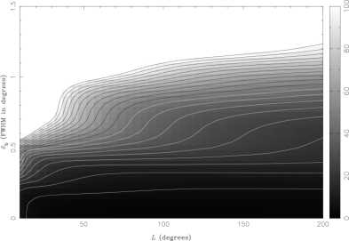
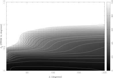
Figure 5: Percentage standard errors in $\Omega$ for $w^{-1}=(15\mu K)^{2}({\rm deg})^{2}$ (top) and $w^{-1}=(30\mu K)^{2}({\rm deg})^{2}$ (bottom). In both cases, isolines are plotted from 5% to 100% at 5% increments.

Clearly, even considering active limited sky coverage, the ideal coverage area is all-sky for the $w^{-1}=(15\mu K)^{2}({\rm deg})^{2}$ case, and also for $w^{-1}=(30\mu K)^{2}({\rm deg})^{2}$, except perhaps for very small beamwidths $\theta_{b}\leq 0.1^{\circ}$. Measuring $\Omega$ as one of a large set of unknown parameters is obviously very sensitive to sample-variance. Even for noise levels that are not too low, like the ones considered, we are dominated by the need to reduce sample variance, not noise.

As explained further in Section 5 there are ambiguities in the covariance matrix approach which allow for some uncertainty in the errors. Thus, in the calculations presented here, we present the most pessimistic results. This resulting error in $\Omega$ is of the order of 20% for $w^{-1}=(15\mu K)^{2}({\rm deg})^{2}$ and $\theta_{b}=0.5^{\circ}$. These errors are quickly reduced to about $5-10\%$ with an improved resolution of $\theta_{b}=0.2^{\circ}$. Therefore a satellite experiment is always ideally scanned with the largest possible sky coverage, and the final result benefits enormously from improving the resolution.

4.2 An intermediate noise deep-patch experiment

If one is observing from the ground, the noise level is always larger. This is because the atmosphere, as well as ground spill-over, acts so as to deteriorate the experiments sensitivity, often by a large factor. If, however, one takes advantage of the fact that a large aperture is no longer a problem, then one may make up for this with increased resolution. The ideal coverage area is now very far from all-sky, but, in any case, a small patch of the sky is more feasible from the ground. We illustrate this promising corner of experiment parameter space in Fig. 6. We have assumed $w^{-1}=(60\mu K)^{2}({\rm deg})^{2}$. A error in $\Omega$ of around 10 percent may then be achieved with a resolution around $0.1^{\circ}$, with a coverage area corresponding to $L=20-40^{\circ}$. It is clear from the figure that, for such an experiment, increasing the coverage area is extremely undesirable.

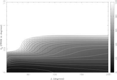
Figure 6: Percentage standard errors in $\Omega$ for $w^{-1}=(60\mu K)^{2}({\rm deg})^{2}$. Isolines are plotted from 10% to 100% in 5% increments.

4.3 An intermediate noise interferometer experiment

In Fig. 7 we show the percentage error in $\Omega$ for an interferometer with a primary beam of $\theta_{w}=4^{\circ}$. We have assumed that a uniform $uv$-plane coverage up to $\ell=1000$ has been achieved by means of a sufficient number of elements, and their arrangement in a suitable geometry. With these assumptions we have then allowed the noise parameter $w^{-1}$ as defined for interferometers to vary between zero and $(100\mu K)^{2}({\rm rad})^{-6}$. Finite sky-coverage errors due to small size and limited number of fields are now substantial. The sample variance in the estimates of $\Omega$ for the interferometer considered can be read off from the $w^{-1}=0$ axis. Although these errors are not small, their limiting values may be approached even for reasonably large values of $w^{-1}$. The need for point-source subtraction typically limits the number of fields, so unfortunately one may not be able to obtain the best result for a given level of noise $w^{-1}$.

We would expect the next generation of CMB interferometer experiments, such as the VSA, VCA and CBI to attain noise level of below $w^{-1}\approx(10\mu K)^{2}({\rm rad})^{-6}$, for the $uv$-coverage assumed above, as compared to $w^{-1}\approx(200\mu K)^{2}({\rm rad})^{-6}$ for the CAT experiment, after foreground subtraction. Assuming a fixed observation time of about 2 years, one could hope to determine $\Omega$ to within about 15–20 percent by observing roughly 20 fields.

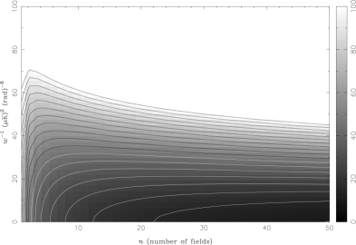
Figure 7: Percentage standard errors in $\Omega$ for an interferometer with $w^{-1}$ up to $(100\mu K)^{2}({\rm rad})^{-6}$. We have assumed a primary beam of $\theta_{w}=4^{\circ}$. Isolines are plotted from 15% to 100% in 5% increments.

5 Dependence on number of undetermined parameters

As one might expected, the number of unknown parameters in a given model has a profound effect on the overall error in determining $\Omega$ (or any other parameter). In this Section we illustrate this important effect, and also highlight some weaknesses in this method of analysis used, particularly in relation to the computation of the curvature matrix.

5.1 Margins of error in covariance matrix estimates

Figure 8: Percentage standard errors in $\Omega$ for an all-sky experiment with $w^{-1}=(15\mu K)^{2}({\rm deg})^{2}$, as one adds more parameters into the problem. The lowest curves consider only $(Q,\Omega)$ to which parameters are then added in the same order as in the full vector ${\bf s}=\{Q,\Omega,$ $\Omega_{b}h^{2},$ $h,n_{S},\Lambda,$ $r,n_{T},\tau,\Omega_{\nu}\}$.

The covariance matrix formalism suffers from an ambiguity in the definition of the derivatives $\partial C_{\ell}/\partial s_{i}$. These have to be computed by means of finite differences, which can never realistically be very small. A particularly difficult derivative is $\partial C_{\ell}/\partial\Omega$. This may be inferred from the approximate formula, valid in the vicinity of sCDM

$$C(\ell,\Omega,h,\Omega_{b}h^{2})\approx C(\ell\Omega^{1/2},1,h\Omega^{1/2},\Omega_{b}h^{2}),$$ (15)

resulting in the relation

$${\partial C_{\ell}\over\partial\Omega}{\Big{|}}_{\Omega=1}={\ell\over 2}{\partial C_{\ell}\over\partial\ell}+{h\over 2}{\partial C_{\ell}\over\partial h}$$ (16)

The effects of $\Omega$ on the plateau can be fitted by a multiplicative factor [5] which has zero derivative at $\Omega=1$, that is, it is a saddle point. Hence the low $l$ signatures of low $\Omega$ models do not appear at all in the linear approximation, in the vicinity of sCDM. Making use of the prescription (16) always results in larger errors than say simply computing the derivative with $\Delta\Omega=.05$. This is not at all surprising, as even such a small difference in $\Omega$ results in a difference in $\ell$ of the order $\Delta\ell\approx\ell\Delta\Omega/2$. This corresponds to taking a finite difference $\Delta\ell$ in (16) which varies with $\ell$ and is always much larger than 1 at large $\ell$. In general increasing the size of the differences used in the computation of the derivatives has the effect of reducing the errors. The reason we bring up this numerical problem is that it may have a physical implication. If the errors are of the order of $10\%$ then it may make more sense to use large finite differences, rather than carefully computed derivatives. Therefore the results presented in the previous sections (where we used very fine grids and also (16)) are to be seen as conservative estimates. A non-linear analysis will always provide smaller errors.

In Fig. 8 we showed the percentage errors in $\Omega$ obtained by two prescriptions for computing the derivatives. On the left we have used the implicit formula (16), on the right we have simply computed a finite difference in $\Omega$. We have also plotted the effects of adding more and more parameters into the problem. The lower curves invert only $\{Q,\Omega\}$. We then add more and more parameters, in the order in which they appear in ${\bf s}$. This picture illustrates the uncertainties inherent in this formalism. It also shows how the errors may change dramatically by adding more and more parameters into the analysis. If one neglects massive neutrinos and uses a finite difference prescription to compute the curvature matrix then an error of 10% in the measurement of $\Omega$ is obtained for $w^{-1}=(15\mu K)^{2}({\rm deg})^{2}$ and $\theta_{b}=0.5^{\circ}$ (as in [4, 5]). By considering one massive neutrino this error goes up to 20% with the same prescription. If instead of using finite differences one computes $\partial C_{\ell}/\partial\Omega$ implicitly, the error goes up to 30%.

5.2 The sample-variance/noise balance and undetermined parameters

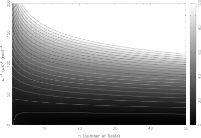
Figure 9: Percentage standard errors in $\Omega$ for an interferometer with $\theta_{w}=4^{\circ}$, considering only the 4 parameters $\{Q,\Omega,$ $\Omega_{b}h^{2},h\}$. Isolines are plotted from 5% to 100% in increments of 5%.

If one assumes the values of some of the parameters, so that fewer of them are allowed to vary, then sample variance naturally becomes less important. In this case, for example, it is no longer necessary to observe such a large number of fields to obtain a successful interferometric determination of $\Omega$. We may illustrate this point by considering the interferometer experiment discussed in the previous section, but this time fixing the values of all but four of the model parameters, and working only with the set $\{Q,\Omega,$ $\Omega_{b}h^{2},h\}$. As shown in Figure 9, with less than 10 fields one could now obtain a better than 5% determination of $\Omega$ for $w^{-1}\approx(10\mu K)^{2}({\rm rad})^{-6}$. Moreover, it is clear that for relatively high noise levels, one could concentrate on a single field, to overcome the instrumental noise, and still obtain a useful result; this is because the sample variance in a single field in this context is only $5-10\%$. Thus, even for $w^{-1}\approx(50\mu K)^{2}({\rm rad})^{-6}$, and for a single field, one could now measure $\Omega$ with an error of about $10-15\%$.

6 Interferometers and other cosmological parameters

Although not central to our discussion, it is interesting to explore the marginal variances for cosmological parameters other than $\Omega$, in particular for interferometers. This is because interferometers may be expected to provide the least noisy estimates of the power spectrum at high $\ell$. Hence the detection of subtle but valuable high $\ell$ signals, such as the acoustic oscillation signature, are obvious goals for such experiments.

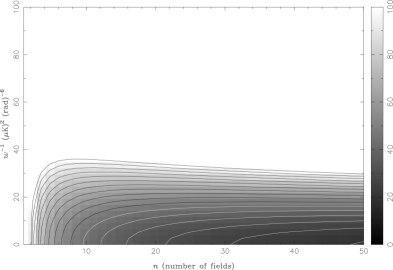
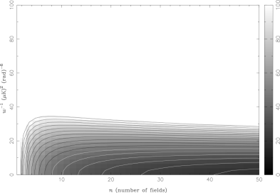
Figure 10: Percentage standard errors in $\Omega_{b}h^{2}$ (top) and $h$ (bottom) for an interferometer with $\theta_{w}=4^{\circ}$, allowing all parameters to vary (but assuming no massive neutrinos). Isolines are plotted from 20% to 100% in increments of 5%.

In Fig. 10 we show the percentage errors in the parameters $\Omega_{b}h^{2}$ (top) and $h$ (bottom), for an interferometer with a primary beam width of $4^{\circ}$, and for which we have allowed all the CDM parameters to vary (but assuming no massive neutrinos). Estimates of the two parameters illustrated in the figure are derived mainly from the relative positions and height of the Doppler peaks in the CMB power spectrum, and it is clear from the figure that a reasonable determination of these parameters is possible. Assuming a noise level of $w^{-1}\approx(10\mu K)^{2}({\rm rad})^{-6}$, the error in both $\Omega_{b}h^{2}$ and $h$ is about 35%, even assuming such a large parameter set. As discussed above, however, these errors can be greatly reduced if the values of some of the other parameters, such as $n_{s}$ or $\Lambda$, can be fixed by other means.

7 Ideal scales away from the vicinity of sCDM

So far we have concentrated our attention on the errors associated in estimating $\Omega$ (and other parameters), assuming the sCDM values for the model parameters. In this section, we conclude by making a brief investigation of how the errors in the determination of $\Omega$ may be much larger if the universe is not described by the sCDM model.

In particular, we will consider two non-standard CDM models which illustrate two ways in which the problem of measuring $\Omega$ may be more difficult. The first is an open universe with $\Omega=0.3$, which has all other model parameters set to their sCDM values; we call this model oCDM. If the signal is of this type then the ideal scales for weighing the Universe will be at much larger $\ell$. Consequently more stringent bounds will be put on the resolution of single-dish experiments. Interferometers, however, will be little affected.

Our second model has $\Omega=1$, but instead we assume a scalar tilt of $n_{S}=0.8$. The remaining parameters all have their sCDM values, and we call this model tCDM. For this type of model the intensity of the signal at the Doppler peaks is much smaller, requiring larger sensitivities from both inteferometers and single-dish experiments. This obstacle for an accurate measurement of $\Omega$ occurs also for signals coming from theories with low $Q$, non-zero $r$ (a gravitational wave component), or non-zero $\tau$ (late reionization).

7.1 Satellite experiments

In Fig. 12 we plot the percentage errors in $\Omega$ for oCDM (top) and tCDM (bottom), for a satellite experiment with $w^{-1}=(30\mu K)^{2}({\rm deg})^{2}$.

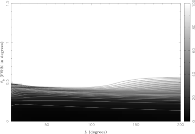
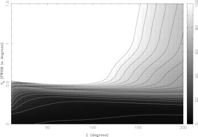
Figure 11: Percentage standard errors in $\Omega$ for a satellite experiment with $w^{-1}=(30\mu K)^{2}({\rm deg})^{2}$ in a universe with all parameters equal to those of sCDM, but with $\Omega=0.3$ (top) and $n_{S}=0.8$ (bottom). Isolines are plotted from 5% to 100% (top) and from 10% to 100 % (bottom), in increments of 5%.

It is clear from the figure that for oCDM we require a resolution of better than $0.4^{\circ}$ in order to determine $\Omega$ to any reasonable accuracy. Overall in comparison with sCDM the error plot gets squashed towards lower $\theta_{b}$. This is what one would expect, since the Doppler peaks in such a model are shifted to significantly higher multipoles, and so a finer angular resolution is required to determine their position. For sufficiently fine resolution and with this relatively low level of noise, we also see that all-sky coverage is now not a great advantage. This is because the sample variance on the CMB power spectrum at the position of the Doppler peaks is reduced by their shift to higher multipoles. In any case, however, for a resolution of $0.1^{\circ}$, one could hope to achieve an accuracy of better than 5%, with little dependence on the area of sky covered.

For tCDM, by comparing the bottom panels of Figs 5 and 11, we see that again the errors are much larger. Overall the effect of reducing the power in the Doppler peaks by considering, say, a theory with $n_{S}<1$, is similar to increasing the noise parameter $w^{-1}$. For this reason all-sky coverage is now far from ideal. A 10% determination of $\Omega$ under these conditions would now require a resolution of about $\theta_{b}\approx 0.2^{\circ}$ with an ideal scanning area corresponding to $L\approx 100^{\circ}$.

7.2 Interferometer experiments

We have also investigated the performance of interferometer experiments in these two non-standard cosmologies, and the results are given in Fig. 12.

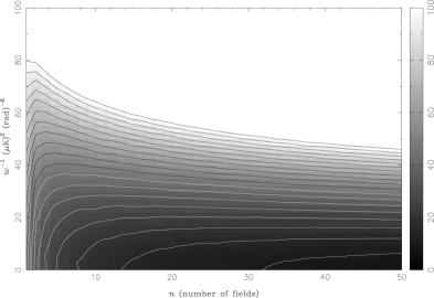
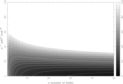
Figure 12: Percentage standard errors in $\Omega$ for the interferometer experiment with $\theta_{w}=4^{\circ}$, for a model with all parameters equal to those of sCDM, but with $\Omega=0.3$ (top) and $n_{S}=0.8$ (bottom). Isolines are plotted from 10% to 100% (top) and 10% to 100% (bottom) in increments of 5%.

From the figure we see that interferometers suffer far less in oCDM than satellite experiments. In fact, there is very little change in the accuracy to which $\Omega$ can be measured. If anything the situation improves wherever interferometers are limited by their large sample variance. This is not surprising, since the $uv$-coverage is assumed constant up to $\ell\approx 1000$. This still easily includes the relevant Doppler peaks in this model. Therefore the noise factor in the sensitive sections of the spectrum does not increase in the same way as it does for a single dish experiment. As an example, for $w^{-1}\approx(50\mu K)^{2}({\rm rad})^{-6}$, we can expect an accuracy of about 15–20% by observing 10–20 fields.

In the tCDM model, interferometers are affected in the same way as single-dish experiments. Again one suffers from a weaker Doppler peak signal, effectivelly similar to a larger noise parameter. Nevertheless, for $w^{-1}\approx(10\mu K)^{2}({\rm rad})^{-6}$ with 20 observed fields, the error in $\Omega$ is still around 20%.

8 Summary and concluding remarks

In this paper we reused the linear approximation tools developed in [4, 5] in a broader context. We considered a larger class of experiments, more evasive signals, and formalism implementations producing less spectacular results. We then set off looking for the ideal experiment for weighing the Universe. The exercise is clearly somewhat naive. Political forces are more likely to determine experimental design than scientific reasons. Nevertheless it is interesting to note from our plots that accurate measurements of $\Omega$ may be expected even from poorly designed experiments.

In a rough summary we found three corners in experiment parameter space which, for different reasons, and using different strategies, provide estimates for $\Omega$ with useful errorbars. Satellite experiments make use of their low noise and intermediate resolution to map the first peak (and maybe part of the second) very accurately. They rely on beating sample variance by means of a large sky coverage. Ground-based and balloon borne experiments may make up for their larger noises with improved resolutions. This results in a better mapping of the second and maybe third Doppler peak. Small-sky coverage is used as a strategy to beat noise. The resulting increase in the sample variance is expected to be less of a problem given the larger $\ell$ at which the relevant measured features occur. Both these experimental strategies suffer dramatically if the Doppler peaks happen to be at larger $\ell$ than in the standard model, such as is the case with open models.

Interferometers constitute a third viable avenue. They may be expected to map the first peak very poorly, but they will do outstandingly well in mapping the secondary peaks, even when compared with high-resolution single-dish experiments. Again a small coverage area technique is employed so as to reduce the effects of noise. The sample variance is always large, but again one may hope that its practical effects are small due to the high $\ell$ features which should be targeted. However, this is not always the case, and in fact interferometers are often limited by sample variance. For this reason experimental interferometric parameters exist, for which performance is improved if the relevant features are at higher $\ell$, as with open models. All this seems to indicate that one should explore more than one experimental avenue in order to avoid unpleasant surprises.

We conclude with a couple of remarks on how to improve the linear analysis performed here. Clearly one should compute the likelihood directly from the $C_{\ell}(s_{i})$ function. This is feasible but computationally demanding. Typically the non-linear analysis tends to predict smaller errors. Also one should go beyond the uniform prior assumption used here. A variety of information on all of the $s_{i}$ parameters exists, coming from all sorts of other sources. This should be incorporated in the priors, naturally reducing the errors of the final estimates. For instance we have found errors in $\Omega_{\nu}$ of order 0.9. These clearly are not compatible with what we already know about the mass of the neutrinos, should there be a heavy neutrino. The same can be said for some of the errors found for $\Omega_{b}$, $h$, $n_{S}$. The final analysis waiting to be done should therefore not only go beyond the linear approximation, but also proceed to set up priors incorporating the vast amount of information coupled to the parameter determination problem posed by the CMB.

In closing we should mention that marginal variances may be perhaps somewhat misleading. We have used them simply because they allow for a nicer display of results. However errorbars are in fact ellipsoids in the parameter space $\{s_{i}\}$. In the non-linear approximation they become rather irregular bubbles of maximum likelihood. Such bubbles cannot be visualized but they encode all the information one may extract from a given experiment. Their computation and storage may turn out to be computationally very demanding, but such is the task one should perform when data finally starts pouring in.

References

- [1] J.Bond and G.Efstathiou, MNRAS 226 655 (1987).
- [2] R. Crittenden, J.R. Bond, R.L. Davis, G.P. Efstathiou and P.J. Steinhardt, Phys. Rev. Lett 71 324-327 (1993).
- [3] L.Knox, Phys.Rev. D52 4307 (1995).
- [4] G. Jungman, M. Kamionkowski, A. Kosowsky and D. Spergel, astro-ph/9507080, to be published in Phy.Rev.Lett. (1996).
- [5] G. Jungman, M. Kamionkowski, A. Kosowsky and D. Spergel, to be published in Phys.Rev. D.
- [6] Hu W., Sugiyama N., Astroph. J. 444 489 (1995); Hu W., Sugiyama N., Phys. Rev. D 51 2599 (1995).
- [7] See http://map.gsfc.nasa.gov.
- [8] See http://astro.estec.esa.nl:80/SA-general/Projects/Cobras/cobras.htlm.
- [9] J.Magueijo and M.Hobson,Cosmic Microwave Background experiments ideally suited for testing the coherence of the underlying cosmological theory, submitted.
- [10] M.Hobson and J.Magueijo, Observability of secondary Doppler peaks by cosmic microwave background experiments with small fields, to be published in MNRAS.
- [11] A. Gould, Astrophys. J. Lett. 440, 510 (1995).
- [12] Press P. H., Teukolsky S. A., Vettering W. T., Flannery B. P., 1994, Numerical Recipes. Cambridge Univ. Press, Cambridge.
- [13] W.N.Brandt, C.R.Lawrence, A.C.S.Readhead, J.N.Pakianathan, and T.M.Fiola, Ap. J. 424, 1 (1994).
- [14] S.Dodelson, astro-ph/9512021.
- [15] Tegmark M., 1996, MNRAS, in press
- [16] U.Seljak and M.Zaldarriaga, astro-ph/9603033.
- [17] E.Keto, The shapes of cross-correlator interferometers, Lawrence Livermore Nat. Lab. Preprint.
- [18] Scott P.F., Saunders R., Pooley G., O’Sullivan C., Lasenby A.N., Jones M., Hobson M.P., Duffett-Smith P.J., Baker J., 1996, ApJ, L1.
- [19] The VSA proposal: see http:mrao.