Evolution of the Galaxy Population Based on Photometric Redshifts in the Hubble Deep Field

Abstract

This paper presents the results of a photometric redshift study of galaxies in the Hubble Deep Field (HDF). The method of determining redshifts from broadband colors is described, and the dangers inherent in using it to estimate redshifts, particularly at very high $z$, are discussed. In particular, the need for accurate high-$z$ spectral energy distributions is illustrated. The validity of our photometric redshift technique is demonstrated both by direct verification with available HDF spectroscopic data and by comparisons of luminosity functions and luminosity densities with those obtained from $z<1$ spectroscopic redshift surveys. Evolution of the galaxy population is studied over $0\lesssim z<4$. Brightening is seen in both the luminosity function and the luminosity density out to $z\approx 3$; this is followed by a decline in both at $z>3$. A population of $z<0.5$ star-forming dwarfs is observed to M${}_{\rm F450W_{AB}}=-11$. Our results are discussed in the context of recent developments in the understanding of galaxy evolution.

1 INTRODUCTION

The study of galaxy evolution is a fundamental but difficult problem in cosmology. Only recently have relatively large surveys, even at modest and intermediate redshifts ($0.2\lesssim z\lesssim 1.5$), been carried out (e.g., Lilly et al. (1995); Cowie et al. (1996); Ellis et al. (1996); Glazebrook et al. 1995b ; Yee, Ellingson, & Carlberg (1996)). Lilly et al. (1995) and Ellis et al. (1996) have studied the galaxy luminosity function (LF) and shown that it evolves over $0\lesssim z\lesssim 1$. Lilly et al. report that the LF for red galaxies does not evolve significantly over $0\lesssim z\lesssim 1$, and conclude that a population of red massive objects must have already been “in place” by $z\approx 1$. On the other hand, their blue subsample is evolving, which indicates that its member galaxies formed later than those in the red subsample. Out to somewhat higher redshifts ($z<1.6$) Cowie et al. (1996) have observed a population of actively star-forming, massive galaxies, and have also found evidence for “downsizing”— a trend in which more massive galaxies appear to be forming at higher redshifts. Morphological studies (Schade et al. (1995); Schade et al. (1996)) show that disks brighten with increasing redshift, indicating a higher rate of star formation in the past. Quite recently, a number of large, star-forming galaxies have been discovered at high redshifts ($z\approx 3$), either serendipitously (e.g. Yee et al. (1996)), or as part of targeted searches (e.g. Steidel et al. 1996a ). These high-redshift objects could very well be the progenitors of present-day typical massive galaxies. These and other clues (see Fukugita, Hogan, & Peebles (1996) for a recent review) hint at a scenario in which massive galaxies formed at $z\approx 3$, and were then followed by a sequence of less and less massive galaxies forming at lower and lower redshifts, leading down to the formation of dwarfs at recent ($z<0.5$) epochs.

To obtain a more definitive and complete picture of the star formation history of galaxies requires systematic surveys covering the full redshift range from the epoch of galaxy formation to the present. At higher redshifts such an investigation is difficult and time-consuming, as galaxies are faint and spectroscopic features difficult to observe. Until recently, known high-redshift galaxies were atypical objects characterized by unusual activity such as strong radio emission (McCarthy (1993)). More indirectly, one often relies on Lyman and metal-line absorption systems which are assumed to be the progenitors of present-day disks and spheroids (e.g. Lanzetta, Wolfe, & Turnshek (1995)). The current numbers of relatively normal, spectroscopically observed galaxies at high redshifts ($z\approx 3$) is still small (e.g., Steidel et al. 1996a ). However, the combination of very deep multi-color images and the photometric redshift technique can provide a relatively easier and less time-consuming way of exploring the high-redshift universe and the evolution of galaxies.

The Hubble Deep Field (HDF) is a very deep set of four-band imaging exposures of a “random” high galactic latitude field (Williams et al. (1996)). The images were obtained by the Hubble Space Telescope (HST) at the end of 1995 and were made available to the community shortly thereafter. Because of its extreme depth (limiting F814W_AB magnitude $>28$), wide wavelength coverage (3000–8000Å), and excellent spatial resolution, the HDF affords an unprecedented opportunity to study the galaxy population to unmatched lookback times.

The redshifts of objects seen in the HDF are of great importance to studies of galaxy evolution, and extensive programs of spectroscopic observations have been undertaken in order to secure them (e.g. Cohen et al. (1996); Moustakas, Zepf, & Davis (1996)). Unfortunately, because of the HDF’s extreme depth, spectroscopic redshifts are not practical for all but the brightest objects in that field. One can, however, use the colors of galaxies to estimate their redshifts with a fair degree of confidence. This color-, or photometric-, redshift technique (e.g. Loh & Spillar (1986); Connolly et al. (1995)) allows the determination of redshifts for HDF objects too faint to be spectroscopically accessible. A number of authors have recently applied the photometric redshift technique to the Hubble Deep Field. Lanzetta, Yahil, & Fernández-Soto (1996) have used color redshifts to identify protogalaxy candidates at $z>5$. At slightly lower redshifts, Gwyn & Hartwick (1996) ($z<5$) and Mobasher et al. (1996) ($z<3$) have used their photometric redshifts to generate luminosity functions. In this paper we present our photometric redshift measurements and then study the luminosity function and luminosity density evolution to $z=4$. Our results differ markedly from those in the Gwyn & Hartwick and the Mobasher et al. studies.

In Section 2 we briefly describe the data and the photometric measurements. We then discuss the determination of photometric redshifts (Section 3) and the possible pitfalls along the way (Section 4). Using what we consider to be our most reliable photometric redshifts, we go on to compute the luminosity function (Section 5) and luminosity density (Section 6), and discuss the observed evolution in the context of a specific current picture of galaxy formation (Section 7). Throughout this paper we assume a flat, matter dominated universe ($q_{0}=0.5,\ \Omega_{0}=1$) with $H_{0}=100\ h\ {\rm km\ s^{-1}\ Mpc^{-1}}$. We use $h=1$ if not otherwise indicated.

2 DATA

The HDF has been observed in four broadband filters (F814W, F606W, F450W, and F300W; central wavelengths of 8140, 6060, 4500, and 3000Å respectively). We used publicly available Version 2 images of the HDF. These images have been processed using the drizzling technique and have a pixel size of 0.04 arcsec (Williams et al. (1996)). We chose to work in the AB system (Oke & Gunn (1983)), using the STScI zero-points given by Ferguson (1996). We used the three Wide Field Camera images which we trimmed because image quality degrades significantly near the edges; all told, the angular area used was 4.48 arcmin².

We performed object finding and photometry using the PPP faint galaxy photometry package (Yee (1991)). Automatic object finding was done in both the F814W and F606W frames, with the results edited by eye and then combined into a single catalog; 1620 objects were thus detected to our F814W_AB completeness limit of $28.0$. Of these 1620, 43 were morphologically classified as stars and were not included in any subsequent analysis. At faint apparent magnitudes many objects are detected in fewer than all four HDF filters; the fraction of objects detected in all four bands is 500/529, 891/1003, and 1289/1577 for objects brighter than F814W${}_{\rm AB}=$ 26, 27, and 28, respectively. We confined our analysis to objects with F814W${}_{\rm AB}\leq 27$.

Because accurate determination of galaxy colors is essential if one is to use them to determine redshifts, we briefly outline the way in which photometry is done in PPP. PPP analyzes the flux growth curves and determines an “optimal aperture” for each filter. Since, of the four HDF bands, the F606W images are the deepest, the F606W flux within the optimal aperture is used to derive the fiducial “total magnitude” of the object. The object’s color is determined using a “color aperture”, which is the smallest of (1) the optimal aperture for that given filter, (2) the F606W optimal aperture, and (3) an aperture of 1.56$"$ (39 pixels) diameter. The above procedure ensures that the measurement of the spectral energy distribution of an object is done over an identical angular area in the four bands. The color aperture (which is generally smaller than the optimal aperture) is used to improve the signal-to-noise ratio in the measurement of the object’s color. “Total magnitudes” for the other three filters are then obtained by correcting the F606W magnitude with the measured colors. Strictly speaking, this procedure will produce the “correct” total magnitudes for the other filters only if there is no color gradient in the galaxy. However, we note that the uncertainty introduced by this procedure is small for most galaxies relative to the total photometric uncertainty. Typical photometric uncertainties at F814W${}_{\rm AB}=27$ are 0.10, 0.09, 0.17, and 0.45 in F814W_AB, F606W_AB, F450W_AB, and F300W_AB respectively.

Ironically, object finding in the HDF may suffer from too large a lookback time and too high a resolution. It is a matter of contention whether a small object in the vicinity of a large galaxy is classified as an individual faint galaxy, or as a fragment or HII region belonging to the nearby parent (see Colley et al. (1996)). Since the presence of substructures misclassified as faint galaxies could affect our results, we inspected the environments of faint ($26<{\rm F814W_{AB}}<27$) objects. It was found that, in our catalog, $\sim 70$% of these objects have absolutely no large companions. Of the remaining $\sim 30$%, most appear to be associated with larger objects only in projection. Even if as many as $\sim 30$% of faint objects are indeed components of larger galaxies, the decrease in the faint galaxy numbers is insufficient to significantly affect our results.

3 DETERMINATION OF REDSHIFTS

3.1 Color Redshifts

The redshift of a galaxy can be estimated by comparing its observed broadband spectral energy distribution (SED) with a set of template SEDs for galaxies at different redshifts and of different spectral types. The technique, termed “photometric” or “color redshifts,” can be thought of as very-low-resolution spectroscopy. Various implementations of the technique have been applied to both cluster and field galaxies at $z<1$ (e.g. Loh & Spillar (1986); Connolly et al. (1995); Belloni et al. (1995)).

As Connolly et al. (1995) point out, the spectral feature that is most important for determining the photometric redshift of a galaxy at $z<1$ is the 4000Å break. The size of the break and the curvature of the spectrum to either side of it carry information about the galaxy’s spectral type. Because of the HDF’s expected redshift depth ($z>1$) and UV coverage, spectral breaks other than those seen at rest-frame optical wavelengths will be important. In particular, the 912Å Lyman break will redshift into the F300W filter at $z\approx 2.3$. Features at $\sim$3646Å (the Balmer break), $\sim$2800Å (due to Mg II), and $\sim$2635Å (due to Fe) will also play a role, particularly in older stellar populations. In Section 4 we examine the effects that misidentification of the various spectral breaks may have on the redshifts measured and the conclusions subsequently reached regarding galaxy evolution.

3.2 Measurement of Redshifts and Spectral Types

We determine the best-fitting redshift and spectral type for each HDF object by comparing its colors against those of a set of templates spanning a range of redshifts (0–5) and spectral types (star-forming through old stellar population). The construction of template colors for the HDF is hampered by the fact that at $z>1$ one observes rest-frame UV regions of the objects of interest—regions for which spectral energy distributions are poorly known even for local galaxies, but which may suffer strong internal reddening. A second complication is that at high $z$ the UV flux is further suppressed through absorption by intergalactic gas (e.g. Madau (1995)).

3.2.1 Technique

We constructed templates in the following way: We used the SEDs of Coleman, Wu, & Weedman (1980; hereafter CWW) which we augmented with two very blue SEDs. The CWW SEDs are a collection of empirical SEDs of representative local galaxies ranging from E to Im in spectral type, and covering wavelengths from 1500 to 10000Å. We extended these SEDs below 1500Å as follows: For spectral types E and Sbc the extension is a power-law extrapolation of the 1500–2500Å region of the SED. For spectral types Scd and Im we extrapolated a power law as for the earlier spectral types, but then replaced it with a GISSEL model spectral shape which has been normalized to that power law extrapolation; the aim of this replacement was simply to reproduce the 912Å break which should be quite prominent in the later spectral types, but which would not be reproduced in a simple power-law extrapolation. The two very blue SEDs with which we augment the CWW set were generated from the GISSEL library and represent young, star-forming galaxies; specifically, we used the constant star formation rate models with a Salpeter IMF (masses $0.1M_{\sun}<M<125M_{\sun}$) and ages of 0.5 and 0.05 Gyr. These two very blue SEDs were added because there are, even locally, substantial numbers of galaxies which are bluer than the bluest CWW type.

We then interpolated between our extended CWW SEDs to cover the spectral-type range more finely. To predict the observed SEDs for a given redshift, we applied the Lyman continuum and line blanketing suppression of the UV flux due to intervening Lyman-forest and Lyman-limit absorbers (Madau (1995)). Finally, template colors were constructed by convolving our modified CWW SEDs with the HST instrumental response curves. At the end of this process we have a set of templates as a function of redshift and spectral type. We will from now on refer to this template set as the “extended CWW” set. It is this template set which was used to generate the redshifts utilized in the analyses of Sections 5 and 6.

The extended CWW template set described above assumes that the spectrum of a galaxy of a given spectral type does not evolve with time. This assumption is obviously questionable considering that at redshifts of interest the universe is only a fraction of its present age. A straightfoward way to treat the problem of the evolving SED would have been to use, as Gwyn & Hartwick (1996) did, spectral evolution models such as the GISSEL library. However, spectral synthesis models do not account for a galaxy’s internal absorption which is particularly important in the UV (see Section 4). Furthermore, there are considerable differences amongst the SEDs predicted by differrent spectral synthesis models (see Charlot, Worthey, & Bressan (1996)). For these reasons we chose not to use spectral synthesis models as templates, preferring instead the non-evolving, empirical CWW spectra.

We note, however, that early in galaxy formation the SEDs of all spectral types are dominated by massive stars and consequently are well represented by late spectral type CWW SEDs. As a galaxy ages due to the aging of its stellar population, its SED will migrate across the range of CWW SEDs from later to earlier spectral types. If the galaxy is actively star-forming, then its SED will of course remain similar to a late-type CWW SED. Consequently, our extended CWW templates can be thought of as corresponding to stellar populations of different ages rather than to different galaxy morphological types. We therefore believe that our extended CWW SEDs are a fair representation of real-life evolving SEDs.

We used $\chi^{2}$ fitting to find the best-matching redshift and spectral type for each HDF object. For each template we calculated

$$\chi^{2}=\sum_{i}\left[{\frac{F_{observed,i}-s\cdot F_{template,i}}{\sigma_{i}}}\right]^{2}.$$ (1)

Here, $F_{observed,i}$ is the flux observed in a given filter $i$ and $\sigma_{i}$ is its uncertainty; $F_{template,i}$ is the flux of the template in the same filter. The scaling term $s$ normalizes the template to the observed SED, and the sum is taken over all four HDF filters. The best-matching redshift and spectral type are obtained by minimizing $\chi^{2}$ as a function of template and $s$. Recall that some objects (112/1003) were detected in fewer than all four filters. Such objects were fitted using the upper bound on the object’s flux: it was assumed that $F_{observed}$ and $\sigma_{observed}$ were both equal to the 1$\sigma$ detection limit for that object and filter and the fit was done as before.

3.2.2 Results

In Figure 1 we compare our photometric redshifts against 74 HDF spectroscopic redshifts available from various sources (Hogg (1996); Steidel et al. 1996a ; Phillips (1996)). The agreement is good with a scatter of $\sigma_{z}=0.12$ for the $z<1.5$ objects, increasing to $\sigma_{z}=0.28$ for those at $z>2$. The catastrophic failure rate is small, with only 2 out of 55 $z<1.5$ objects being assigned anomalously high photometric redshifts.

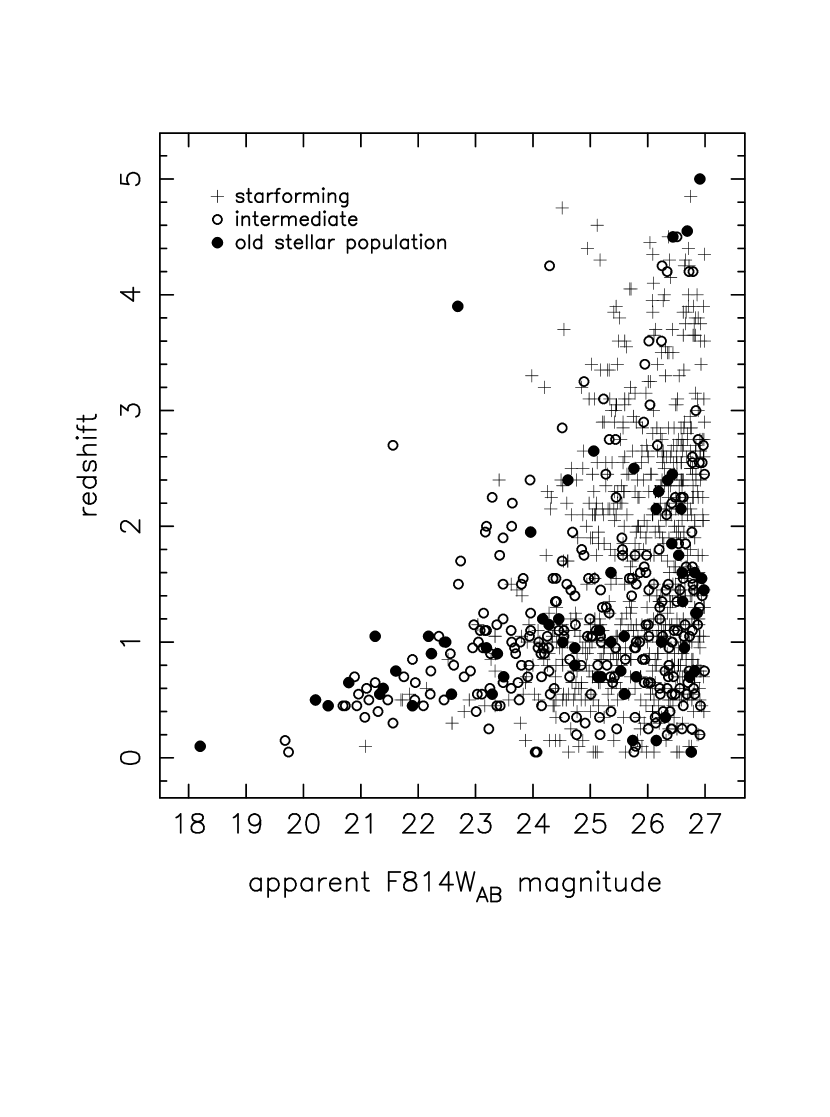
Figure 2: The Hubble Diagram for the HDF. Different symbols correspond to ranges of spectral types: filled circles are galaxies with an old stellar population, open circles are objects with intermediate ages, and crosses denote star-forming galaxies.

Figure 2 shows the Hubble diagram for the HDF. The different symbols refer to different spectral types: filled circles denote spectral types with an old stellar population (CWW E through other early SEDs), open circles are objects with stellar populations of intermediate age (CWW Sbc through Scd) while crosses are star-forming objects (CWW Im through the two very blue SEDs). We draw attention to the presence, at $4<z<5$, of a small number of objects with early spectral types. We regard these objects as low-redshift galaxies whose redshifts have been aliased (see Section 4) to high redshifts because of the confusion between the 4000Å and 912Å breaks.

Figure 3 presents the redshift distribution of the HDF galaxies (thick line) for two apparent limiting magnitudes. The sample is also split by spectral type. Note that there is a prominent peak at $z\lesssim 1$ which is strongly dominated by star-forming galaxies (dashed line) at faint magnitudes (top panel). A second population of star-forming galaxies can be seen at $z\approx 2$–$2.5$ in the top panel of Figure 3. Though there is a slight increase in the overall number of galaxies at $z\approx 2.2$, the very large high-$z$ peak reported by Gwyn & Hartwick (1996) is not seen in our analysis.

4 REDSHIFT ERRORS

The photometric redshift technique will determine an incorrect redshift when the colors of an observed galaxy match the colors of a “wrong” template more closely than they match those of the “right” one. Such aliasing may happen for three reasons: (1) random photometric errors, (2) a template set that is too sparse, and (3) a template set produced with unrealistic SEDs.

Aliasing of templates produces errors which are either minor or dramatically catastrophic. Minor redshift errors (such as most of the redshift discrepancies seen in Figure 1) are best described as “noise” and are relatively benign. The size of this noise is on the order of $\sigma_{z}=0.1$–$0.3$ as can be seen in Figure 1. If need be, the effect of the redshift noise can be modeled (as is done in Section 5) by means of Monte Carlo simulations.

Catastrophic errors can, however, have a profound effect on the conclusions one reaches regarding galaxy evolution (as will be illustrated in Section 4.3) and so we turn to investigate their nature more closely.

4.1 Effects of Random Photometric Errors

If the colors of an observed galaxy are similar to the colors of two templates, then random photometric errors may tip the scales in favor of one or the other of the templates. If the two templates have vastly different redshifts, one of them right and one wrong, then the observed object may be assigned a catastrophically erroneous redshift.

One might expect the fraction of objects scattered from low redshift to high redshift to be the same as that scattered from high redshift to low redshift. However, the number of objects scattered from low redshift to high redshift is likely to be much larger than that scattered in the opposite direction since one can expect there to be many more objects (down to a certain apparent magnitude) at low redshift than at high redshift.

The importance of this type of redshift aliasing depends on the size of photometric uncertainties. Monte Carlo simulations show that catastrophic aliasing of redshifts in the HDF is insignificant for bright objects and starts to become noticeable only at F814W${}_{\rm AB}\approx 27$ at the 10% level. It is for this reason that we limit our analysis to objects brighter than F814W${}_{\rm AB}=27$.

4.2 Effects of a Sparse Template Set

Aliasing of redshifts may also occur when the template set is sparse. If templates at the correct redshift are placed too far apart (i.e. too sparsely) in spectral type, then it may happen that a template with a catastrophically wrong redshift matches the observed SED more closely than does either of the two best-matching templates at the correct redshift. In such a case the wrong redshift (and possibly spectral type) will be chosen. In addition to the spectral type dimension, the template set can also be too sparse in the redshift dimension. Likewise, the same sparseness problem may occur if the template normalization term ($s$ in equation(1)) with too coarse a step size is used in the fitting.

The sparseness aliasing problem can be easily avoided by using sufficiently many intermediate spectral types, redshifts, and steps in $s$. In particular, we used 81 spectral types, redshift steps of 0.05, and $s$ steps of 0.1 magnitude. Decreasing the sparseness of the template set further had no effect on the redshifts and spectral types that were measured.

4.3 Effects of an Unrealistic Template Set

The photometric redshift technique is likely to identify the correct redshift and spectral type provided the grid of templates includes a template which is at the correct redshift and matches the observed colors of the galaxy. If, however, the “correct” template is not included in the template set, an erroneous redshift and spectral type may be chosen. As Connolly et al. (1995) point out, the photometric redshift “signal” (at low redshift) comes from the 4000Å break. As we noted earlier, other spectral breaks exist at 3656Å, $\sim$2635Å, $\sim$2800Å, and 912Å. Since strong spectral breaks are primary sources of signal for identifying photometric redshifts, one can expect that there will be ambiguity between the various breaks and, hence, the corresponding redshifts. One then has to rely on the relative break sizes and on spectral curvature to identify the correct redshift. If the template set being used is erroneous in the sense that the break sizes and spectral curvatures do not model those in real galaxies, one may well be systematically identifying incorrect redshifts.

4.3.1 The Cause

UV spectra are not well known even for local galaxies. Since it is in the rest-UV that one observes extremely high redshift galaxies, one has to be concerned about the effect that this will have on the correctness of one’s template set.

The problem is compounded further because galaxies evolve on timescales comparable to the look-back times that one hopes to probe in the HDF. One could hope to include the effects of spectral evolution by using spectral synthesis models such as the GISSEL library (Bruzual & Charlot (1993)). Such models, however, simulate the naked stellar populations and do not include the effects of galactic self-absorption which may strongly depress the flux blueward of $\sim$1500Å. Furthermore, there is still considerable disagreement between the various spectral synthesis models (see Charlot, Worthey, & Bressan (1996)). This disagreement is serious enough that templates constructed using different models may give catastrophically different photometric redshifts.

It is for these reasons — uncertainty in evolutionary SED codes and their lack of internal reddening — that we have chosen to base our analysis on photometric redshifts obtained using templates that are based on local galaxy spectra (i.e. the “extended CWW” set).

Yet another factor which can contribute to making one’s template set unrepresentative is intergalactic hydrogen. This hydrogen, which resides in Lyman-$\alpha$ clouds, will suppress UV flux through continuum absorption and line blanketing (Madau (1995)). If one neglects to account for this absorption, one will end up with an unrealistic template set even if the input SEDs otherwise match those of real high-redshift galaxies.

4.3.2 The Effect

To illustrate the effect that our poor knowledge of UV SEDs may have on the values of photometric redshifts, we compare the redshifts obtained using our “best model” — the extended CWW — with those obtained using a template set based on pure GISSEL models. We took the ($\Omega=1$) reference models of Pozzetti, Bruzual, & Zamorani (1996) which are GISSEL SEDs chosen to match local E/S0, Sab-Sbc, Scd-Sdm, and “very blue” (rapidly star-forming) objects. In every respect (other than Lyman absorption which we did not apply) we have processed the pure GISSEL SEDs of Pozzetti, Bruzual, & Zamorani (1996) in exactly the same way as in the case of the extended CWW SEDs.

The pure GISSEL template set makes no correction for internal absorption, nor does it account for high-$z$ Lyman absorption. Even though Gwyn & Hartwick (1996) used evolving SEDs they noted that using present-day SEDs made no difference to their results. We therefore assume that our pure GISSEL template set is similar to the template set used by Gwyn & Hartwick (1996). Photometric redshifts in the HDF were then computed with the pure GISSEL template set, in the same fashion (same $z$ and $s$ step sizes) as those that were obtained with the extended CWW template set.

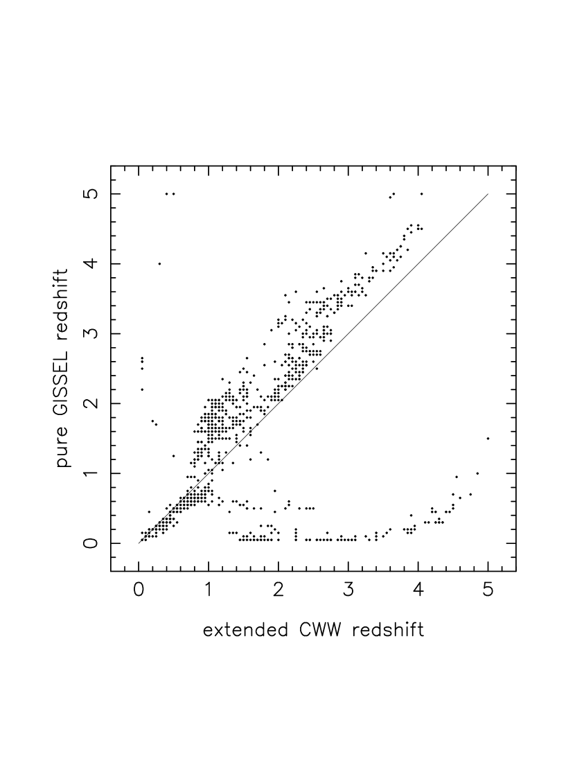
Figure 4: Comparison of photometric redshifts obtained using a pure GISSEL template set with those obtained using our “best model” extended CWW templates. The pure GISSEL template set accounts for neither internal reddening nor high-$z$ Lyman absorption, both of which suppress the UV flux.

Figure 4 compares the photometric redshifts obtained using the pure GISSEL templates described above with those obtained using our extended CWW set. The two template sets produce similar results up to $z\approx 0.8$ but then diverge considerably. This divergence can be attributed to aliasing between spectral breaks — the 4000Å break (giving a lower redshift in the extended CWW fits) and a combination of Balmer, $\sim$2800Å, and $\sim$2635Å breaks (giving the higher redshifts in the pure GISSEL fits). Overall, only 55% of redshifts obtained using the two template sets are within 0.5 of each other. We believe that the extended CWW template set produces more accurate redshifts, since, in contrast to the pure GISSEL set, it accounts for the presence of reddening and Lyman absorption.

In addition to drastic differences in redshift, the two different template sets assign completely different spectral types. In Figure 5 we present the redshift distribution obtained using the pure GISSEL templates. This redshift distribution is characterized by two prominent peaks, in contrast to the redshift distribution shown in Figure 3. The redshift distribution subdivided by spectral type is also shown, using the same convention as in Figure 3. Note that the majority of $z>1$ objects in Figure 5 are identified as early-type, in drastic contrast to Figure 3. This difference arises because the spectrum of an unreddened old stellar population (i.e. an early type galaxy) at $z\approx 1.8$ looks very similar, under the coarse resolution afforded by broadband filters, to that of a reddened, Lyman-suppressed, star-forming galaxy at $z\approx 1.2$. Again, as with the determination of redshift, we believe that the extended CWW templates are more realistic and will produce more accurate spectral types.

In the case of the pure GISSEL results the conclusion likely to be drawn is that at $z\approx 2$ there exists a large population of old galaxies. In contrast, results based on extended CWW templates favor no such radical conclusion. Clearly, the true shape of galaxy SEDs in the UV can have profound effects on the redshifts and spectral types that one fits and, consequently, on the conclusions that are reached regarding galaxy evolution.

4.4 Our Best Template Set and the Redshifts it Produces

We have limited ourselves to F814W${}_{\rm AB}\leq 27.0$ which ensures that aliasing due to photometric errors is insignificant. We have interpolated finely enough in SED, redshift, and normalization (the $s$ of equation (1)) to ensure that template sparseness is not a concern. The third source of possible aliasing is the uncertainty in the UV SEDs, especially of high redshift galaxies. There is not much that can be done here other than to say that by using empirical template SEDs we are accounting for internal reddening, and that by including the high-$z$ Lyman absorption we are accounting for intergalactic hydrogen. We also draw attention to the fact that we recover the redshifts of the great majority of objects for which spectroscopic redshifts exist (see Figure 1). We are prepared to trust the validity of our results out to $z\approx 3.5$. We have little confidence in any redshifts at $z>4$, as there are no spectroscopic redshifts there with which we can verify our photometric ones.

Armed with some degree of confidence in the photometric redshifts obtained with the extended CWW templates, we now proceed to compute the luminosity functions and luminosity densities of galaxies in the HDF.

5 LUMINOSITY FUNCTIONS

The luminosity function (LF) is a standard and basic way of describing the galaxy population. Using the redshift catalog obtained with the extended CWW template set (Section 3), we now turn to investigate the galaxy population and its evolution by means of luminosity functions. To determine the LFs we use a maximum likelihood method (see, e.g., Efstathiou, Ellis, & Peterson (1988) and Lin et al. (1997) for more details). This method is insensitive to fluctuations in galaxy density — an important feature in a pencil-beam survey such as the HDF. To facilitate comparison with $z<1$ results our LFs are computed in the rest-frame F450W${}_{\rm AB}\approx B_{\rm AB}$ band. We fit the LF to the usual Schechter (1976) parametrization and list the fit parameters ($M^{*},\alpha$, and $\phi^{*}$) in Table 1.

Our sample has constant apparent magnitude limits and yet covers an enormous baseline in redshift. A consequence of the enormous redshift range is the large K-corrections which effectively remove red objects out of the sample at high redshift. On the other hand, blue, star-forming galaxies have much smaller K-corrections and do not suffer from this effect. It should be noted, however, that at high enough redshifts one does not expect to see many intrinsically red objects, since at those redshifts the universe may be too young for stellar populations to have aged sufficiently.

5.1 Comparison with $z<1$ Spectroscopic Surveys

At $z<1$ we can compare our HDF luminosity functions with those obtained from spectroscopic redshift surveys. Figure 6 shows such a comparison with the $B_{\rm AB}$-band LFs derived from the Canadian Network for Observational Cosmology (CNOC; Lin et al. (1997); Lin et al., in preparation) and Canada-France (CFRS; Lilly et al. (1995) ) redshift surveys. The comparison is made against a sample of CNOC galaxies with $0.12<z<0.6$ (1236 objects) and a sample of CFRS galaxies with $0.5<z<1$ (424 objects). The LFs shown in Figure 6 are those for all objects, irrespective of their spectral types. The agreement between the HDF LFs and those from the CNOC and CFRS samples is good over the magnitude range common to the HDF and the spectroscopic survey samples. In this common range the LF shapes from the three samples are similar, showing flat faint-end slopes ($\alpha\approx-1$), though the normalization of the HDF $0.5<z<1.0$ LF is somewhat higher than that of the corresponding CFRS sample.

In the two upper panels of Figure 7 we divide the HDF, CNOC, and CFRS samples into subsamples of galaxies bluer or redder than our CWW Scd model, and then compare the resulting LFs. Our HDF results are again consistent with those derived from the spectroscopic surveys. The agreement between the HDF photometric redshift LFs and those derived from the spectroscopic surveys is very encouraging, and gives us confidence to proceed to fainter objects and to higher redshifts.

5.2 Low-$z$ Faint Galaxies

At absolute magnitudes fainter than those accessible to either CNOC or CFRS, the HDF LF is no longer flat (see Figure 6), but has a much steeper slope ($\alpha\approx-1.3$). This excess of faint galaxies is similar to that seen at $z\approx 0$ in the Center for Astrophysics (CfA) survey (Marzke et al. 1994a ; Marzke, Huchra, & Geller 1994b ) and in the CFRS sample at $z<0.2$ (Lilly et al. (1995)), although the HDF data demonstrate that the excess continues to at least as faint as $M_{{\rm F450W}_{\rm AB}}=-11$.

When we split the LF by spectral type, as in the bottom panel of Figure 7, we see that those faint galaxies which are responsible for the steep $\alpha$ also have the blue late-type colors indicative of ongoing star formation. The same trend was also reported by Marzke et al. (1994a) for their local faint-end excess. About 80% of our sample at $0.2<z<1.0$ are actually bluer than our model extended CWW Scd galaxy.

In principle, the misidentification of HII regions as faint galaxies (Section 2) could cause an artificial steepening of the faint-end slope. However, the rate of misidentifications (30% assuming that all non-isolated faint objects are misclassified HII regions) is too small to negate the existence of the star-forming dwarf excess.

The rather large redshift noise ($\sigma_{z}\approx 0.13$ at these redshifts) could cause an artificial brightening of $M^{*}$ and steepening of $\alpha$ (SubbaRao et al. (1996)). This is an effect akin to one that photometry errors can have on the LF (e.g., Efstathiou, Ellis, & Peterson (1988)). By means of Monte Carlo simulations, we tested the distortion that redshift noise may have on our determination of the LF. Specifically, we generate model redshift catalogs using some given input LF, then perturb these catalogs with Gaussian redshift errors similar to the noise we see in the actual HDF redshift catalog, and finally compute the LF based on the perturbed model catalogs. We find that the effects of redshift errors are small (given the absolute magnitude ranges we fit), with negligible effect on $\alpha$, and slight brightening of $M^{*}$ (a couple tenths of a magnitude). These effects are smaller than the 1$\sigma$ errors we quote in Table 1. In particular, a flat ($\alpha=-1$) input LF cannot steepen to the slope $\alpha=-1.3$ that we actually see in the HDF. We therefore conclude that the steep faint-end slope of our HDF LF is not an artifact of photometric redshift errors. We also verified that the effects of redshift noise on the LF are not important at higher $z$; for simplicity we will not make any corrections for this effect in calculating our luminosity functions.

5.3 Evolution of the Luminosity Function out to $z=4$

We now turn to investigate the evolution of the luminosity function with redshift. The LFs for five redshift bins between $z=0.2$ and $z=4$ are shown in Figure 8. The LFs have not been split by color but we note that the galaxies at higher redshifts are almost exclusively blue, star-forming objects. Schechter function fits to the LFs are shown as lines and the fit parameters are listed in Table 1. The $0.2<z<0.5$ (dashed line) and $1<z<2$ (dotted line) fits are used as fiducials.

The LFs presented in Figure 8 show clear signs of evolution with redshift. The bright end of the LF appears to brighten by $\sim 0.5$ mag from $0.2<z<0.5$ to $1<z<2$, and by a further $\sim 0.5$ mag from $1<z<2$ to $2<z<3$. The faint end slope steepens considerably with lookback time, from $\alpha=-1.3$ at $0.2<z<0.5$ to $\alpha=-2$ at $2<z<3$. The HDF LF thus appears, almost monotonically, to both brighten and steepen in shape with increasing lookback time, up to $z\approx 3$. The most drastic change occurs between the $2<z<3$ and $3<z<4$ redshift bins, as there we see the LF fade back to values similar to those seen at low redshift. We interpret this fading as consistent with the view that the majority of present-day $\sim L^{*}$ galaxies began star formation around that time, as we elaborate in Section 6.

We note that we do not see the $\sim 5$ magnitude brightening of the luminosity function measured by Gwyn & Hartwick (1996) and Mobasher et al. (1996). The difference arises because both internal reddening (absent from the models of Gwyn & Hartwick 1996) and Lyman absorption (absent from Gwyn & Hartwick 1996 and from Mobasher et al. 1996) suppress the UV flux. In the absence of this suppression galaxies tend to be assigned much earlier spectral types even if their redshifts are identified correctly. Early spectral types require very large K-corrections compared to those needed for late types and consequently tend to be given much brighter absolute magnitudes. This effect manifests itself as an overly strong brightening of the luminosity function.

6 LUMINOSITY DENSITY

6.1 The Luminosity Density of the Universe

We obtain the comoving luminosity density as a by-product of the luminosity function measurements. Figure 9 shows the comoving luminosity densities measured at rest-frame F450W_AB and F300W_AB. The luminosity density in each redshift bin was computed by integrating the corresponding LFs over $-23<M_{\rm F450W_{AB}}<-15$ or $-21<M_{\rm F300W_{AB}}<-15$; the errors were estimated from the standard deviation of the mean of the three Wide Field Camera chips. The values for the $z<1$ luminosity densities obtained by Lilly et al. (1996) from the CFRS at similar wavelengths (4400Å, 2800Å) are also shown, together with their $(1+z)^{\beta}$ parametrizations. Up to $z\approx 3$, the HDF luminosity densities show a monotonic increase in both the rest- F300W and F450W bands, although (at least for the F300W band) not at as high a rate as one would extrapolate from the the CFRS $z<1$ data. The luminosity density peaks in the $2<z<3$ bin and past $z=3$ it drops. These same trends were also seen in the LF evolution illustrated in Figure 8.

It is interesting to interpret the evolving luminosity density in terms of the global star formation history of the universe. We use simple GISSEL models to represent the star formation history of all galaxies within a comoving volume element. In Figure 9 we choose one particular set of models synthesized from the GISSEL library to compare against the observed luminosity densities. The models are those for a stellar population characterized by a Salpeter initial mass function (IMF) ($x=1.35$, $0.1M_{\odot}<M<125M_{\odot}$) in which star formation exponentially declines with a decay time $\tau=2$ Gyr (Bruzual & Charlot (1993)). As in the rest of this paper, we use $q_{0}=0.5$, but here we choose a specific $H_{0}$ value, 45 km s^-1 Mpc^-1, in order to make $t_{0}=14.5$ Gyr. We choose to start the star formation in our models at $t_{f}=1,1.5$, and 2 Gyr after the Big Bang, corresponding to formation redshifts $z_{f}=5.0,3.6$, and 2.8, respectively. The models were arbitrarily normalized by eye to pass between the low-$z$ HDF points (at $0.2<z<1.0$) and the $z<1$ CFRS results.

All three models are quite similar at $z\lesssim 1.5$ and reproduce the observed luminosity density trends well at $z<1$. At high redshifts the $z_{f}=3.6$ model appears to match the observations best. It is intriguing that this simple toy model reproduces, albeit roughly, the bulk features of the observed luminosity density evolution in the HDF, and that it does so in both bandpasses at the same time. In the context of these toy models, the implication of our results is that the bulk of the stellar population of the universe appears to have started forming at $z=3-4$. Clearly, our models are almost certainly an oversimplification of reality, but they do give us a rough handle on the initial epoch of galaxy formation.

6.2 Production of Metals from $z=4$ to the Present

The UV flux from galaxies can be used as a measure of both the star formation rate and the metal production rate (e.g., Cowie (1988); Songaila, Cowie, & Lilly (1990); Cowie et al. (1996)). The metal production rate can be more readily related to the UV flux, with the results independent of cosmology, and relatively independent of the details of galaxy or star formation history or the specific form of the IMF (Cowie (1988)). As an interesting consistency check on the results presented earlier, we investigate the metal density of the universe (inferred from the HDF UV luminosity densities) as a function of redshift.

Songaila et al. (1990) give the relevant relation

$$\frac{\rho Z\ }{10^{-34}\ {\rm g\ cm}^{-3}}=\frac{S_{\nu}\ }{3.6\times 10^{-25}\ {\rm ergs\ cm}^{-2}\ {\rm s}^{-1}\ {\rm Hz}^{-1}\ {\rm deg}^{-2}}\ ,$$ (2)

where $\rho Z$ is the present volume density of metals produced by some population of objects at redshift $z$. $S_{\nu}$ is the present observed surface brightness of those objects at observed frequencies $\nu=\nu_{0}/(1+z)$. The source frequencies $\nu_{0}$ have to lie in a flat (in $f_{\nu}$) part of the source spectrum, which is the case in rest-UV for star-forming galaxies. We can thus transform rest-${\rm F300W}_{\rm AB}$ luminosity densities to presently-observed surface brightnesses, and then infer the present-day density of metals that were produced by these high-$z$ star-forming HDF galaxies.

In Figure 10 we plot (solid line) the cumulative metal density produced by HDF galaxies as a function of $z$. Here we have assumed that the universe was metal-free before $z=4$ (as we do not trust our photometric redshifts beyond $z=4$, we have no constraints there). The bounds on the present-day metal density of the universe, $\rho Z=8-24\ h^{2}$ g cm^-3 (Cowie et al. (1996)), are shown as dashed lines for the Hubble constant $h=0.7$. The lower and upper bounds for $h=0.5$ and $h=1$, respectively, are shown as dotted lines. By $z=0$ the inferred metal density matches the local constraints well, implying that we are indeed seeing in the HDF all the needed metal production. Also shown (open squares) are the metallicity constraints from high-redshift observations of damped Lyman-$\alpha$ systems made by Pettini et al. (1994) and Lu et al. (1996); the large error bars on the data are meant to represent the large spread in metallicity values that is observed. To convert the metallicity measurements to actual metal densities we assumed that the mass density in damped Lyman-$\alpha$ systems at high redshifts is the same as that in present-day stars (Lanzetta, Wolfe, & Turnshek (1995)); that is, that the damped Lyman-$\alpha$ systems are indeed the progenitors of present day galaxies. (Here we also used the central value $h=0.7$.) Keeping the large uncertainties in mind, there is reasonable agreement between the metal densities inferred from the HDF and from damped Lyman-$\alpha$ systems. It is reassuring that the redshift-dependent metal density derived from the F300W_AB luminosity density, which in turn was derived using photometric redshifts, is consistent with both the local and high-redshift metal densities obtained from completely independent measurements.

7 DISCUSSION

As discussed in Section 6.1, our simple GISSEL toy model provides a rough but reasonable match to the observed evolution of the HDF luminosity density. Within the context of this model, the rise in the luminosity density from $z\approx 3.5$ to $z\approx 2.5$ means that the initial major epoch of star formation in galaxies occured at $3<z<4$. Such a picture is certainly consistent with the presence of a population of luminous, star-forming galaxies discovered recently at $z\sim 3$ (e.g., Steidel et al. 1996a ; Yee et al. (1996)). Also, interestingly, the peak in the luminosity density seen in the $z=2$–$3$ bin coincides in redshift with the peaks observed in the number density of bright, optically-selected quasars (e.g. Warren, Hewett, & Osmer (1994)) and radio galaxies (e.g. Dunlop & Peacock (1990)).

Below $z\approx 3$ we see several conspicuous trends in the HDF luminosity density and luminosity function. There is a strong decline in the luminosity density with decreasing redshift. This decline is a reflection of the accompanying marked changes in the LF: the LF is simultaneously fading and flattening at ever lower redshifts, as seen in Figure 8. The flattening of the LF faint-end slope is a characteristic of hierarchichal models of galaxy formation (e.g. Cole et al. (1994)). In our data this flattening appears to be accompanied by moderate fading of the bright end of the LF, perhaps indicating that both merging and luminosity evolution play a role.

As the majority of galaxies we observe in the HDF are star-forming objects, the changes seen in the LF imply a migration in the characteristic luminosities of star-forming galaxies, from brighter at high $z$, to fainter at lower redshifts. If we can roughly associate the $B$-band luminosities of these galaxies with their underlying stellar masses (though it would have been preferrable to have longer rest-wavelength data, such as $K$-band, for this purpose; Cowie et al. (1996)), our LF results suggest that the less massive the galaxy, the more recently it is undergoing a period of strong star formation. This same trend has been observed (and termed “downsizing”) in the spectroscopic survey sample of Cowie et al. (1996) over lower redshifts ($0.2<z<1.7$). Our analysis indicates that this trend extends over the entire redshift range from $z\sim 3$ to the present; the characteristic star-forming galaxy luminosity migrates from the bright end of the LF at $z\sim 3$ to below present-day $M^{*}$ at $z<1$. At $z<0.5$, star-forming galaxies dominate the dwarf population. If star-forming galaxies are indeed in the process of initially assembling themselves, then we may conclude that galaxy formation occured sequentially in size, with the largest objects forming at $z>3$ and the smallest only recently. This picture is consistent with the scenario of galaxy formation reviewed by Fukugita et al. (1996), in which massive spheroidal galaxies formed at $z\approx 3$, followed at later epochs by the formation of less massive objects, and finally by the formation of dwarfs in recent times. That the mass density of neutral gas in damped Lyman-$\alpha$ systems (the likely progenitors of present-day galaxies) appears to decrease rapidly below $z\approx 3.5$ (Lanzetta, Wolfe, & Turnshek (1995)) lends support to the picture that conversion of gas to stars was actively happening below $z\sim 3$. Moreover, as a consistency check on our results, the density of metals inferred from the HDF agrees with the bounds available at both low and high redshifts (Figure 10).

At the lowest redshifts, $z<1$, our luminosity function and luminosity density results agree, within regions of overlap, with results from spectroscopic surveys (Figures 6 and 7). Furthermore, as an extension of the downsizing trend from higher $z$, we see a large population of star-forming dwarfs extending to luminosities below the reach of the current spectroscopic surveys (Figure 7). Such low-redshift bursting dwarfs have been evoked (e.g., Broadhurst, Ellis, & Shanks (1988)) to explain the excess counts of faint blue galaxies. Recent evidence from direct luminosity function measurements (Ellis et al. (1996); Cowie et al. (1996); Lilly et al. (1995)), as well as more indirect morphological studies of deep HST images, including the HDF (e.g., Glazebrook et al. 1995a ; Abraham et al. (1996)), have indicated that the faint blue galaxies are rapidly evolving, star-forming, and have irreguliar or peculiar morphologies. Our direct HDF luminosity function results lend further support to this picture, and also show that the low-$z$ dwarf population reaches very faint luminosities indeed.

Although we have outlined above an overall picture of the star-formation history of the universe, many of the specifics remain to be filled in. Are the LF changes, in particular the steepening of $\alpha$ at higher $z$, due to luminosity-dependent luminosity evolution, or is merging also taking place? What are the individual evolutionary tracks of particular galaxies in the space of luminosity, spectral type, morphology, and other parameters? Will detailed galaxy formation models, which include both galaxy, stellar, and clustering evolution (e.g., Kauffmann, Nusser, & Steinmetz (1995); Baugh, Cole, & Frenk (1996)), be able to account for the clear redshift-dependent changes we observe in the HDF luminosity functions? These and similar questions have not been addressed in the present paper, though we do plan for future work to relate the morphologies of HDF galaxies to the existing LF information, thereby hopefully filling in more of the details in the picture of galaxy evolution.

We caution that our results rely on the validity of photometric redshifts — redshifts whose determination, as has been shown in Section 4, can be fraught with danger. The fact that our redshift determination relies on the poorly constrained UV properties and equally poorly constrained spectral evolution of galaxies is a major cause for concern. Although we have taken many precautions to guard against catastrophic redshift errors, our results and the conclusions that we derive from them can be confirmed only with additional spectroscopic redshift verification.

We thank Bob Williams for assigning Director’s Discretionary Time to the Hubble Deep Field and the HDF team for the data. We also thank David Schade and Gabriela Mallén-Ornelas for useful comments and Nick Kaiser for the encoragement he provided. This research was supported by NSERC of Canada.

Table 1: Parameters of Schechter Function Fits

$z$ range	color sample	$M^{*}_{\rm F450W_{AB}}-5\log h$	$\alpha$	$\phi^{*}$ ($h^{3}$ Mpc-3)	$N$
0.2 – 1.0	all	$-20.1\pm 0.3$	$-1.33\pm 0.05$	$0.033\pm 0.009$	357
0.2 – 1.0	bluer than Scd	$-18.9\pm 0.3$	$-1.3\pm 0.1$	$0.045\pm 0.012$	277
0.2 – 1.0	redder than Scd	$-20.7\pm 0.6$	$-1.1\pm 0.1$	$0.015\pm 0.006$	80
0.2 – 0.5	all	$-21.2\pm 1.6$	$-1.4\pm 0.1$	$0.009\pm 0.007$	103
0.5 – 1.0	all	$-19.9\pm 0.4$	$-1.3\pm 0.1$	$0.042\pm 0.013$	254
1.0 – 2.0	all	$-22.1\pm 0.7$	$-1.6\pm 0.1$	$0.006\pm 0.006$	291
2.0 – 3.0	all	$-23.2\pm 1.5$	$-2.1\pm 0.1$	$0.002\pm 0.004$	198
3.0 – 4.0	all	$-20.4\pm 0.7$	$-1.3\pm 0.3$	$0.023\pm 0.017$	63

Figure 1: Comparison of photometric and spectroscopic redshifts. Photometric redshifts were obtained using our extended CWW template set. A perfect match would lie on the diagonal line.

Figure 3: Redshift distribution of objects brighter than F814W${}_{\rm AB}=27$ (top panel) and those brighter than F814W${}_{\rm AB}=25.5$ (bottom panel). The thick solid line denotes all objects irrespective of spectral type. The dotted line denotes star-forming galaxies, the dashed line denotes objects with intermediate ages, and the thin solid line denotes those with an old stellar population.

Figure 5: Redshift distribution (cumulative and split by spectral type) obtained using pure GISSEL templates which account for neither internal reddening nor high-$z$ Lyman absorption. Symbols are the same as those in Figure 3.

Figure 6: Comparison of HDF luminosity functions with those from the CNOC and CFRS spectroscopic redshift surveys. Top panel: $0.2<z<0.5$. Bottom panel: $0.5<z<1.0$. Solid lines are Schechter function fits to the HDF data; fit parameters are listed in Table1.

Figure 7: HDF luminosity functions split by color. The top two panels compare the HDF LFs with CNOC and CFRS spectroscopic survey results when split into blue (top panel) and red (middle panel) subsamples. The bottom panel compares the relative contributions of galaxies bluer than Scd (filled symbols) and those redder than Scd (open symbols); the solid line is the Schechter function fit to all the $0.2<z<1.0$ HDF objects.

Figure 8: Evolution of the luminosity function with redshift. Solid lines are Schechter function fits to the data. Dashed and dotted lines are fiducial LFs — the dotted line is the $1<z<2$ HDF LF and the dashed line is the $0.2<z<0.5$ HDF LF. Schechter fit parameters are listed in Table 1.

Figure 9: Luminosity density of the universe from the HDF (filled symbols) at rest-4500Å (top panel) and rest-3000Å (bottom panel) . Open triangles are data from Lilly et al. (1996) and the dashed lines are fits (and extrapolations) of these data. Dotted lines are luminosity densities generated from GISSEL models assuming an exponentially decaying burst of star formation (see text for more details), which started at $z_{f}=$ 2.8, 3.6, or 5.0.

Figure 10: The metal density of the universe derived from UV fluxes of HDF objects (filled squares). Open squares are metal densities inferred from metallicities of damped Lyman-$\alpha$ systems. Dashed lines represent bounds on the present-day metal density assuming $h=0.7$; dotted lines are upper and lower bounds assuming $h=1$ and $h=0.5$ respectively (see text for more details).

References

- Abraham et al. (1996) Abraham, R. G., Tanvir, N. R., Santiago, B. X., Ellis, R. S., Glazebrook, K., & van den Bergh, S. 1996, MNRAS, 279, L47
- Baugh, Cole, & Frenk (1996) Baugh, C. M., Cole, S., & Frenk, C. S. Frenk 1996, MNRAS, in press, preprint astro-ph/9602085
- Belloni et al. (1995) Belloni P., Bruzual G., Thimm G.J., Röser H.-J. 1995, A&A, 297, 61
- Broadhurst, Ellis, & Shanks (1988) Broadhurst, T. J., Ellis, R. S., & Shanks, T. 1988, MNRAS, 235, 827
- Bruzual & Charlot (1993) Bruzual A., G., & Charlot, S. 1993, ApJ, 405, 538
- Charlot, Worthey, & Bressan (1996) Charlot, S., Worthey, G., & Bressan, A. 1996, ApJ, 457, 625
- Cohen et al. (1996) Cohen, J. G., Cowie, L. L., Hogg, D. W., Songaila, A., Blandford, R., Hu, E. M., & Snopbell, P. 1996, ApJ, 471, L5
- Cole et al. (1994) Cole, S., Aragón-Salamanca, A., Frenk, C. S., Navarro, J. F., & Zepf, S. E. 1994, MNRAS, 271, 781
- Coleman, Wu, & Weedman (1980) Coleman, G. D., Wu, C.-C., & Weedman, D. W. 1980, ApJS, 43, 393 (CWW)
- Colley et al. (1996) Colley, W. N., Rhoads, J. E., Ostriker, J. P., & Spergel, D. N. 1996, ApJ, in press, preprint astro-ph/9603020
- Connolly et al. (1995) Connolly, A.J, Csabai, I., Szalay, A. S., Koo, D. C., Kron, R. C., & Munn, J. A. 1995, AJ, 110, 2655
- Cowie (1988) Cowie, L. L. 1988, in The Post-Recombination Universe, eds. N. Kaiser & A. N. Lasenby (Dordrecht: Kluwer), 1
- Cowie et al. (1996) Cowie, L. L., Songaila, A., Hu, E. M., & Cohen, J. G. 1996, AJ, in press
- Dunlop & Peacock (1990) Dunlop, J. S., & Peacock, J. A. 1990, MNRAS, 247, 19
- Efstathiou, Ellis, & Peterson (1988) Efstathiou, G., Ellis, R. S., & Peterson, B. A. 1988, MNRAS, 232, 431
- Ellis et al. (1996) Ellis, R. S., Colless, M., Broadhurst, T., Heyl, J., & Glazebrook, K. 1996, MNRAS, 280, 235
- Ferguson (1996) Ferguson, H. 1996, http://www.stsci.edu/ftp/observer/hdf/logs/zeropoints.txt
- Fukugita, Hogan, & Peebles (1996) Fukugita, M., Hogan, C. J., & Peebles, P. J. E. 1996, Nature, 381, 489
- (19) Glazebrook, K., Ellis, R., Santiago, B., & Griffiths, R. 1995a, MNRAS, 275, L19
- (20) Glazebrook, K., Peacock, J. A., Miller, L., & Collins, C. A. 1995b, MNRAS, 275, 169
- Gwyn & Hartwick (1996) Gwyn, S. D. J., & Hartwick, F. D. A. 1996, ApJ, 468, L77
- Hogg (1996) Hogg, D. W. 1996, http://astro.caltech.edu/dwh/deep/hdf.html
- Kauffmann, Nusser, & Steinmetz (1995) Kauffmann, G., Nusser, A., & Steinmetz, M. 1995, MNRAS, submitted, preprint astro-ph/9512009
- Lanzetta, Wolfe, & Turnshek (1995) Lanzetta, K. M., Wolfe, A. M., & Turnshek, D. A. 1995, ApJ, 440, 435
- Lanzetta, Yahil, & Fernández-Soto (1996) Lanzetta, K. M., Yahil, A., & Fernández-Soto, A. 1996, Nature, 381, 759
- Lilly et al. (1996) Lilly, S. J., Le Fèvre, O., Hammer, F., & Crampton, D. 1996, ApJ, 460, L1
- Lilly et al. (1995) Lilly, S. J., Tresse L., Hammer, F., Crampton, D., & Le Fèvre, O. 1995, ApJ, 455, 108
- Lin et al. (1997) Lin, H., Yee, H. K. C., Carlberg, R. G., & Ellingson, E. 1997, ApJ, in press, preprint astro-ph/9608056
- Loh & Spillar (1986) Loh, E. D., & Spillar, E. J. 1986, ApJ, 303, 154
- Lu et al. (1996) Lu, L., Sargent, W. L. W., & Barlow, T. A. 1996, ApJS, in press, preprint astro-ph/9606044
- Madau (1995) Madau, P. 1995, ApJ, 441, 18
- (32) Marzke, R. O., Geller, M. J., Huchra, J. P., & Corwin, H. 1994a, AJ, 108, 2
- (33) Marzke, R. O., Huchra, J. P., & Geller, M., J. 1994b, ApJ, 428, 43
- McCarthy (1993) McCarthy, P. J. 1993, ARA&A, 31, 639
- Mobasher et al. (1996) Mobasher, B., Rowan-Robinson, M., Georgakakis, A., & Eaton, N. 1996, MNRAS, submitted, preprint astro-ph/9604118
- Moustakas, Zepf, & Davis (1996) Moustakas, L., Zepf, S., & Davis, M. 1996, http://astro.berkley.edu/davisgrp/HDF
- Oke & Gunn (1983) Oke, J. B., & Gunn, J. E. 1983, ApJ, 266, 713
- Pettini et al. (1994) Pettini, M., Smith, L. J., Hunstead, R. W., & King, D. L. 1994, ApJ, 426, 79
- Phillips (1996) Phillips, D. 1996, http://www.ucolick.org/deep/hdf/zlist hdf.txt
- Pozzetti, Bruzual, & Zamorani (1996) Pozzetti, L., Bruzual A., G., & Zamorani, G. 1996, MNRAS, in press, preprint astro-ph/9604087
- Schade et al. (1996) Schade, D., Carlberg, R. G., Yee, H. K. C., López-Cruz, O., & Ellingson, E. 1996, ApJ, 465, L103
- Schade et al. (1995) Schade, D., Lilly, S.J., Crampton, D., Hammer, F., Le Fevre, O., Tresse, L. 1995, ApJ, 455, L1
- Schechter (1976) Schechter, P. L. 1976, ApJ, 203, 297
- Songaila, Cowie, & Lilly (1990) Songaila, A., Cowie, L. L., & Lilly, S. J. 1990, ApJ, 348, 371
- (45) Steidel, C. C., Giavalisco, M., Dickinson, M., & Adelberger, K. 1996a, AJ, in press, preprint astro-ph/9604140
- (46) Steidel, C. C., Giavalisco, M., Pettini, M., Dickinson, M., & Adelberger, K. 1996b, ApJ, 462, L17
- SubbaRao et al. (1996) SubbaRao, M. U., Connolly, A. J., Szalay, A. S., & Koo, D. C. 1996, AJ, in press, preprint astro-ph/9606075
- Warren, Hewett, & Osmer (1994) Warren, S. J., Hewett, P. C., & Osmer, P. S. 1994, ApJ, 421, 412
- Williams et al. (1996) Williams, R. E., Blacker, B., Dickinson, M., Van Dyke Dixon, W., Ferguson, H. C., Fruchter, A. S., Giavalisco, M., Gilliland, R. L., Heyer, I., Katsanis, R., Levay, Z., Lucas, R. A., McElroy, D. B., Petro, L., Postman, M., Adorf, H.-M., & Hook, R. N. 1996, AJ, in press, preprint astro-ph/9607174
- Yee (1991) Yee, H. K. C. 1991, PASP, 103, 396
- Yee et al. (1996) Yee, H. K. C., Ellingson, E., Bechtold, J., Carlberg, R. G., & Cuillandre, J.-C. 1996 AJ, 111, 1783
- Yee, Ellingson, & Carlberg (1996) Yee, H. K. C., Ellingson, E., & Carlberg, R. G. 1996 ApJS, 102, 269