MPI-PhT/96-48

AN ICOSAHEDRON-BASED METHOD FOR PIXELIZING THE CELESTIAL SPHERE

Max Tegmark

Max-Planck-Institut für Physik, Föhringer Ring 6, D-80805 München;

Max-Planck-Institut für Astrophysik, Karl-Schwarzschild-Str. 1, D-85740 Garching;

email: max@ias.edu

For power spectrum estimation it’s important that the pixelization of a CMB sky map be smooth and regular to high degree. With this criterion in mind the “COBE sky cube” was defined. This paper has as central theme to further improve on this elegant scheme which uses a cube as projective base - here an icosahedron is used in its place. Although the sky cube is excellent, a further reduction of 20 percent     of the number of pixels can be obtained while the pixel distance is maintained, and without any degradation of accuracy for integration. The pixels are rounder in this scheme where they are hexagonal rather than square, and the faces are small in this implementation which simplifies area-equalization. The reason distortion is lessened is that the faces are smaller and therefore more flat. To use the method, you can get a FORTRAN code from the Internet.

1 INTRODUCTION

In astronomy and cosmology, this is the age of map-making. Recent ground-based and satellite-borne experiments have produced all-sky maps at a wide range of wavelengths, spanning from radio frequencies to the infra-red, ultraviolet and x-ray bands. Although the brightness distributions being measured are always continuous functions of position, the maps are in practice compiled and distributed with values only at some finite number of points, or pixels. As discussed below, a good choice of pixelization scheme can often substantially simplify the subsequent analysis of the data, and for this reason, considerable amounts of work have been spent on developing good schemes for pixelizing the celestial sphere. Arguably the best and most elaborate method to date is the so-called COBE sky cube scheme (Chan & O’Neill 1976, O’Neill & Laubscher 1976), which has been successfully employed for the DMR, DIRBE and FIRAS maps of the COBE satellite. This method has a number of desirable properties, and it is rather obvious that it cannot be radically improved upon. However, the next generation of cosmic microwave background (CMB) maps from instruments such as the MAP and COBRAS/SAMBA satellites will be subjected to very extensive and time-consuming processing in order to obtain measurements of cosmological parameters. In view of this, it is timely to search for still better pixelization schemes, since even quite modest improvements can translate into substantial numerical gains. The purpose of this Letter is to present such an improved method for pixelizing the sphere, akin to the sky cube method but replacing the cube by an icosahedron.

1.1 What is a “good” pixelization?

What do we mean by a pixelization scheme being good? Specifically, if we are to place $N$ points (pixel centers) on the sphere, where is the best place to put them? We will use the following two criteria:

1. The worst-case distance to the nearest pixel should be minimized.

2. We should be able to accurately approximate integrals by sums.

Defining $d$ as the maximum distance that a point on the sphere can be from the pixel closest to it, criterion 1 says to minimize $d$. Criterion 2 states that the integral of a function over the sphere should be well approximated by $(4\pi/N)$ times the sum of the function values at the pixel locations. This is important for applications such as CMB maps, where one wants to expand the brightness distribution in some set of functions, e.g., spherical harmonics. Intuitively, we expect that both of these goals can be attained if the pixel distribution is in some sense as regular as possible. So if $N=6$, for instance, one might opt for the 6 corners of a regular octahedron. Unfortunately, there is only a finite number of platonic solids (SO(3) has only a finite number of discrete subgroups), so there is in general no obvious “most regular” pixelization scheme.

1.2 The icosahedron advantage

The COBE sky cube pixelization scheme is illustrated in Figure 1 (top), and consists of the following steps:

1. The sphere is inscribed in a cube, whose faces are pixelized with a regular square grid.

2. The points are mapped radially onto the sphere.

3. The points are shifted around slightly, to give all pixels approximately equal area.

A pixel (the area which is closer to a given point than to all other points) is thus approximately square, with a side of length $\sim\sqrt{4\pi/N}$. The points furthest from the pixels lie at the corners of these squares, so

$$d_{cube}\approx\sqrt{2\pi\over N}.$$ (1)

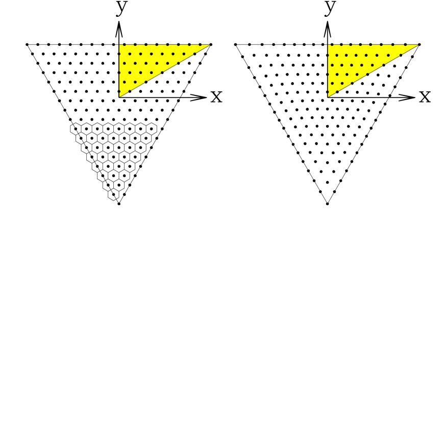
Figure 2: A regular triangular grid (left) is adjusted (right) to give all pixels the same area. As illustrated, the pixels have a hexagonal shape. A triangular icosahedron face can be symmetrically decomposed into six identical right triangles (one is shaded), and the area equalization mapping is seen to respect this symmetry.

For a honeycomb grid as illustrated in Figure 2, a pixel is hexagonal, and one readily computes that

$$d_{icosa}\approx\sqrt{8\pi\over 3\sqrt{3}N},$$ (2)

a value which is about $12\%$ smaller than that for the square grid case. To take advantage of this, one could thus replace the sky cube by a Platonic solid with triangular faces, i.e., by the tetrahedron, the octahedron or the icosahedron.

The above-mentioned area-equalization is carried out for the sake of our second criterion, loosely speaking so that the equal weights that the pixels get when summed over correspond to equal weights $d\Omega$ in an integral (we present a rigorous application of criterion 2 in the discussion section). Since the pixels originally were on a rectangular grid on the cube faces (on the the tangent plane of the sphere), the amount of “stretching” required increases toward the edges of the faces. Both this and the radial projection makes the pixels slightly deformed, so that the further out on a face one goes, the more the corresponding pixels on the sphere depart from a regular grid. Because of this, it is clearly desirable to use as small faces as possible, so that the corresponding regions of the sphere are as flat as possible. The Platonic solid with the smallest faces is the one with the largest number of faces: the icosahedron, whose faces are 20 triangles (see Figure 1). Not only does it have the advantage of having more than three times as many faces as the cube, which one would expect to help with criterion 2, but since the faces are triangles rather than squares, it is better according to criterion 1 as well. These advantages led Ned Wright to make an independent implementation of the icosahedron scheme in the early 1980’s, with an area-equalization that was approximate rather than exact.

The rest of this Letter is organized as follows. The icosahedron-based pixelization method is described in Section 2 and numerically compared with the COBE sky cube method in Section 3.

2 METHOD

The icosahedron pixelization scheme is illustrated in Figure 1 (bottom), and is akin in spirit to the COBE sky cube method:

1. The sphere is inscribed in an icosahedron, whose faces are pixelized with a regular triangular grid.

2. The points are mapped radially onto the sphere.

3. The points are shifted around slightly, to give all pixels approximately equal area.

A FORTRAN package implementing this is available at
h t t p://www.sns.ias.edu/$\tilde{~{}}$max/icosahedron.html
(faster from the US) and from
h t t p://www.mpa-garching.mpg.de/$\tilde{~{}}$max/icosahedron.html
(faster from Europe).
The user interface is identical to that for the COBE sky cube package: for any specified resolution, one subroutine converts a pixel number to a unit vector, and a second subroutine converts a unit vector to a pixel number, the number of the pixel closest to that vector. Below we merely summarize the geometrical issues that specify the method.

2.1 Part I: mapping to and from the icosahedron

The 3D aspects of the problem are computationally trivial, since any of the 20 icosahedron faces can be rotated to lie in the $z=1$ plane by multiplication by an appropriate rotation matrix, and all these rotation matrices can be precomputed once and for all. The mapping between the $z=1$ tangent plane and the surface of the unit sphere preserves the direction of a vector and simply changes its length appropriately, either to be unity (on the sphere) or to have $z=1$. It is easy to see that straight lines on the tangent plane correspond to great circles on the sphere. Thus each icosahedron face gets mapped onto a region on the sphere bounded by three great circles.

2.2 Part II: the area equalization

The area equalization step is illustrated in Figure 2. After mapping part of the sphere onto a triangle in the tangent plane as above, we want to map this triangle onto itself (“shift the pixels around”) in such a way that the combined mapping becomes an equal-area mapping, i.e., gets a constant Jacobian. The Jacobian of the mapping from the sphere to the plane is

$$\left|{\partial(x,y)/\partial\Omega}\right|=(1+x^{2}+y^{2})^{3/2},$$ (3)

so we want to find find a second mapping $(x,y)\mapsto(x^{\prime},y^{\prime})$ whose Jacobian is proportional to the inverse of this. In other words, we wish to find two functions $(x^{\prime},y^{\prime})$ that map the boundary of the triangle onto itself and satisfy the nonlinear partial differential equation

$$\det\left(\matrix{\partial x^{\prime}/\partial x&\partial x^{\prime}/\partial y\cr\partial y^{\prime}/\partial x&\partial y^{\prime}/\partial y\cr}\right)=\eta^{2}(1+x^{2}+y^{2})^{-3/2}$$ (4)

for some proportionality constant $\eta$. Since the icosahedron has 20 faces, the area of the triangular region on the sphere is clearly $4\pi/20$. The sides of the equilateral triangle in the tangent plane have length $a=\left[9\tan^{2}\left({\pi\over 5}\right)-3\right]^{1/2}\approx 1.323$, so its area is $a^{2}\sqrt{3}/4$. Taking the ratio of these two areas fixes the above proportionality constant to be

$$\eta=\left[{15\sqrt{3}\over 4\pi}\left(3\tan^{2}{\pi\over 5}\,-\,1\right)\right]^{1/2}\approx 1.098.$$ (5)

The partial differential equation equation (4) is under-determined and admits infinitely many solutions, which allows us to impose additional simplifying requirements. As illustrated in Figure 2, the triangle can be decomposed into six right triangles of identical shape that can all be mapped into the one in the upper right corner (shaded) by a combination of $120^{\circ}$ rotations and reflections. We require our solution to respect this symmetry, so we merely need to find a solution to equation (4) in the shaded triangle that maps its boundary onto itself. We use the additional freedom to require that horizontal lines in this region get mapped onto horizontal lines. This is enough to determine the solution uniquely, and we find that

$$\cases{y^{\prime}&$=\eta\sqrt{{2\over\sqrt{3}}\tan^{-1}\left[\sqrt{3}{\sqrt{1+4y^{2}}-1\over\sqrt{1+4y^{2}}+3}\right]}$,\cr\vskip 4.0pt\cr x^{\prime}&$=\left({\eta xy^{\prime}\over y}\right)\sqrt{1+4y^{2}\over 1+x^{2}+y^{2}}$,}$$ (6)

which can be verified by direct substitution. These equations are readily inverted, giving

$$\cases{y&$={1\over 2}\sqrt{3\left[{1+\sqrt{3}\tan(\sqrt{3}y^{\prime 2}/2\eta^{2})\over\sqrt{3}-\tan(\sqrt{3}y^{\prime 2}/2\eta^{2})}\right]^{2}-1}$,\cr\vskip 4.0pt\cr x&$=x^{\prime}y\sqrt{{1+y^{2}\over y^{\prime 2}(1+4y^{2})-x^{\prime 2}y^{2}}}$.}$$ (7)

This area-equalizing mapping is illustrated in Figure 2, where the regular triangular grid of points (left) has been adjusted (right) to give equal-area pixels when projected onto the sphere. The pixels in Figure 1 have also been equal-area adjusted — otherwise a slight excess would be visible near the corners of the triangles.

3 DISCUSSION

We have presented a new method for pixelizing the sphere, devised to be useful for storing and analyzing all-sky maps in astronomy and cosmology, and made a FORTRAN implementation publicly available over the Internet.

As far as practical issues goes, it is essentially equivalent to the COBE sky cube method: the pair of subroutines that convert between unit vectors and pixel numbers are for all practical purposes instantaneous. How does its geometric performance compare with that of the COBE sky cube method according to the two criteria described in the introduction? As discused, the fact that the pixels are hexagons rather than squares reduces the maximum distance to the grid by about $10\%$. With respect to criterion 1, it is easy to see that hexagonal pixels are optimal on a flat surface, so they clearly cannot be substantially improved upon for the sphere either when $N$ is large. In addition, rounder pixels are of course appealing since the instrumental beam tends to be round. We will now examine criterion 2 in more detail, and find that in a certain well-defined sense, the improvement of the icosahedron method when integrating is about $10\%$ as well.

3.1 Spherical Cubature

The study of how to best approximate integrals with sums has a long tradition in the mathematics literature. For instance, the famous quadrature formula of Gauss shows how a 1-dimensional integral $\int_{a}^{b}f(x)dx$ can be approximated with a weighted average $\sum_{i=1}^{N}w_{i}f(x_{i})$ such that the approximation becomes exact if $f$ is a polynomial of degree less than $2N$. That this is plausible can be readily seen by noting that there are $2N$ free parameters (the positions $x_{i}$ and the weights $w_{i}$) available to satisfy the $2N$ constraints. When integrating on a circle rather than an interval, the Gauss problem becomes greatly simplified, and a simple Fourier expansion shows that exactness for polynomials of degree less than $2N$ is obtained by the most naive prescription possible: $N$ equispaced points with equal weights (as compared with the zeroes of the Legendre polynomials in the Gauss case). In other words, the 1-D interval case appears to have been complicated by the presense of endpoints, whereas in the fully symmetric case, the optimal scheme was that where the pixelization was as regular as possible. Since the sphere also lacks endpoints that break symmetry, one might therefore conjecture that the optimal integration formula would involve a maximally regular pixelization and equal weights. Unfortunately, it is a well-known group-theoretical result that there are no completely regular point distributions on the sphere for $N>20$. This has led to an extensive body of work on the problem of optimal integration on the sphere — see e.g. Stroud (1971), Sobolev (1974), Konjaev (1979) and Mysovskikh (1980) for theoretical work on this so-called cubature problem. Although no strictly optimal method has been found for general $N$ (which is one of the main foci of the mathematics literature, together with proofs of various bounds on how well one can do), we will see that from a pragmatic astrophysicist’s point of view, the icosahedron scheme is so close to optimal that further improvements may not be worthwhile.

We can clearly write our approximation of the integral $\int fd\Omega$ as $\int wfd\Omega$, where the weight function $w(\widehat{\bf r})$ is a linear combination of $N$ delta-functions. Let us define the integration error as

$$\Delta\equiv\sum_{i=1}^{N}w_{i}f(\widehat{\bf r}_{i})-\int f(\widehat{\bf r})d\Omega=\int[w(\widehat{\bf r})-1]f(\widehat{\bf r})d\Omega.$$ (8)

The cubature problem thus involves finding a $w$ that makes $\Delta$ vanish when $f$ is any polynomial up to a given degree. We see that this is equivalent to finding a $w$ that is orthogonal to all such polynomials except the monopole (which gives the integral). As an orthonormal basis for distributions on the sphere, let us select the Gram-Schmidt orthogonalized polynomials. This basis is simply the spherical harmonics $Y_{\l m}$, where $\l$ gives the degree of the polynomials ($\l=1$ gives linear functions, $\l=2$ gives harmonic quadratic polynomials, etc.). A useful way to diagnose any integration scheme is thus to compute the spherical harmonic coefficients of $w$,

$$w_{\l m}\equiv\int Y_{\l m}^{*}(\widehat{\bf r})w(\widehat{\bf r})d\Omega=\sum_{i=1}^{N}w_{i}Y_{\l m}^{*}(\widehat{\bf r}_{i}),$$ (9)

and plot its window function $W_{\l}$, defined as

$$W_{\l}\equiv\sum_{m=-\l}^{\l}|w_{\l m}|^{2}.$$ (10)

Such histograms are plotted in Figure 3 for the COBE sky cube method and the icosahedron method using a comparable number of points, both with all weights $w_{i}=4\pi/N$. Apart from the monopole (which gives the integral), both are seen to vanish for all polynomials of degree $\l\ll 100$, which means that these methods are essentially exact in Gauss’ sense to that order. Comparing the two methods, the icosahedron scheme is seen to remain accurate out to approximately $10\%$ greater $\l$-values, so in this sense, the method is about $10\%$ better. This gain factor was found be remain around $10\%$ over the range of $N$-values likely to be of astrophysical interest.

How close to optimal is the icosahedron method? Although a rigorous lower bound for general $N$ has still not been proven, an approximate answer can readily be found by simple constraint-counting as with the Gaussian quadrature case above. There are $\l^{2}$ spherical harmonics of degree less than $\l$, whereas $w$ is specified by $3N$ free parameters ($N$ weights $w_{i}$ and $N$ unit vectors $\widehat{\bf r}_{i}$). One might thus hope to obtain a perfect window function up to $\l\approx\sqrt{3N}$, i.e., to make the integration exact for polynomials of degree up to $\sqrt{3N}$. For the examples in Figure 3, we have $\sqrt{3N}\approx 136$ and $137$, respectively, i.e., values quite close to where the icosahedron window function becomes substantial. The problem of finding a strictly optimal solution has been attacked numerically (Schmid 1978), but the nonlinear system of equations involved was found very difficult to solve in practice for large $N$. Moreover, from the point of view of a pragmatic astrophysicist, it is not even clear that such a solution would be better than those in Figure 3, since there is no guarantee that its window function does not explode uncontrollably for $\l>\sqrt{3N}$. If the mapped signal has some angular power spectrum $C_{\l}$, then the mean square integration error is readily seen to be

$$\langle\Delta^{2}\rangle=\sum_{\l=1}^{\infty}W_{\l}C_{\l}.$$ (11)

In astrophysics applications, the signal power spectrum typically falls off smoothly around the scale set by the beam width of the observing instrument, so the mathematical problem of making $W_{\l}$ exactly zero while ignoring $W_{\l+1}$ altogether is clearly not physically motivated. Rather, the astrophysicists concern is simply that $W_{\l}\approx 0$ well beyond the beam smoothing scale, and then grows in a controlled way.

Finally, it should be emphasized that these integration-related issues are crucial for the next generation of cosmic microwave background maps, since they will be integrated against a large number of weight functions in order to obtain accurately power spectrum measurements. Since the data processing in these applications involves matrix algebra where the computational cost scales as $N^{3}$ (Bunn & Sugiyama 1995; Tegmark et al. 1996), even modest reductions in the number of pixels translate into substantial savings in CPU time and storage requirements. For instance, a $12\%$ better window function allows $25\%$ fewer pixels, which corresponds to halving the CPU time.

Given the great efforts that will be spent on collecting and analyzing such data sets, there should be no reason to use anything but the best scheme when pixelizing the data. We have found that the icosahedron method improves upon the COBE sky cube method by about $10\%$ when it comes to both integration accuracy and worst-case distance to the nearest pixel center. Since this improvement is computationally speaking free, it is hoped that the icosahedron method will be useful for future mapping experiments.

The author wishes to thank James Binney, Angélica de Oliveira-Costa, Vikram Seth, Harold Shapiro and Ned Wright for useful comments, and Schwabinger Krankenhaus for hospitality during the visit where this work was carried out. This work was partially supported by European Union contract CHRX-CT93-0120 and Deutsche Forschungsgemeinschaft grant SFB-375.

4 REFERENCES

Bunn, E. F. & Sugiyama N. 1995, ApJ, 446, 49.

Chan, F.K. & O’Neill, E.M. 1976, Feasibility study of a quadrilateralized spherical cube Earth data base, Computer Sciences Corp. EPRF Technical Report.

Konjaev, S. I. 1979, Mat. Zametki, 25, 629.

Mysovskikh, I. P. 1976, in Quantitative Approximation, eds. R. A. Devore & K. Scherer (New York: Academic Press).

O’Neill, E.M. & Laubscher, R.E. 1976, Extended studies of a quadrilateralized spherical cube Earth data base, Computer Sciences Corp. EPRF Technical Report.

Schmid, H. J. 1978, Numer. Math., 31, 281.

Sobolev, S. L. 1974, Introduction to the theory of cubature formulae (Moscow: NAUKA).

Stroud, A. H. 1971, Approximate Calculation of Multiple Integrals (Englewood Cliffs: Prentice-Hall).

Tegmark, M., Taylor, A. & Heavens, A. F. 1996, preprint astro-ph/9603021.

Figure 1: The cube-based and icosahedron-based pixelization schemes.

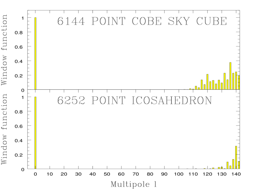
Figure 3: Window function comparison. The histograms show the errors obtained when approximating integrals by sums, multipole by multipole. The icosahedron method generally remains accurate down to about $10\%$ smaller scales than a COBE sky cube with a similar number of pixels, which means that it can produce comparable results using about $20\%$ fewer pixels.