Abstract

We describe the Bayesian-based signal-to-noise eigenmode method for cosmological parameter estimation, show how it can be used to optimally compress large CMB anisotropy data sets to manageable sizes, and apply it to the DMR 4-year, South Pole and Saskatchewan data, individually and in combination. A simple prior probability method is used to include large scale structure observations. Estimates of the Hubble parameter, vacuum energy density, baryon fraction and primordial spectral tilt derived from the combined data are given.

COSMIC PARAMETER ESTIMATION COMBINING SUB-DEGREE CMB EXPERIMENTS WITH COBE

¹ Canadian Institute for Theoretical Astrophysics, Toronto, Ontario, Canada. ² Center for Particle Astrophysics, UC Berkeley, Berkeley CA USA.

1 Introduction

As CMB anisotropy experiments have gotten more ambitious, our need for powerful statistical methods has become more urgent. For the CMB data sets that have been obtained up to now, including COBE [1] (dmr4), the 1994 South Pole data of [2] (sp94) and the 1993-95 Saskatoon data of [3, 4] (sk95), which we analyze jointly here, it is possible to do a relatively complete Bayesian statistical analysis if the primary anisotropies are assumed to be Gaussian and the non-Gaussian Galactic foregrounds are not large. Even for these experiments, this is feasible only because of compression, in which the data set is acted upon by linear operators which project it onto subspaces of the full data. In the past the linear combinations of the data were defined by what made intuitive sense (e.g., weighted sums of different frequency channels or weighted averages of pixel separations below the beam scale), and could still leave too many pixels to deal with in a complete analysis. Here we use the rigorous signal-to-noise eigenmode approach to data compression [5] to reduce the sets to the manageable $\mathrel{\hbox to0.0pt{\lower 3.0pt\hbox{$\mathchar 536\relax$}\hss}\raise 2.0pt\hbox{$\mathchar 316\relax$}}1000$ important combinations. As we approach the era of megapixel data sets promised by MAP and COBRAS/SAMBA, via the era of tens of thousands of pixels promised by long duration balloon experiments, the question of how to come as near to optimal compression as possible given computer limitations becomes of paramount importance. This happy day of too many pixels is now upon us.

The goal is to estimate the parameters $\{y_{A}\}$ of a target set of theories with angular power spectra ${\cal C}_{{\ell}}$ by first determining the likelihood function ${\cal L}(\{y_{A}\})$ for each theory, and then comparing the likelihoods as a function of the parameters. Using Bayes’ theorem, we can write the probability of the theoretical parameters, given the observations and the class of theories being tested, $P(\{y_{A}\}|{\rm OBS},\,{\rm TH})\propto{\cal L}(\{y_{A}\})P(\{y_{A}\}|{\rm prior})$, where the assumed prior probability distribution $P(\{y_{A}\}|{\rm prior})$ can reflect a priori maximal ignorance, or take into account constraints from other information such as large scale structure observations. The proportionality constant is related to the probability that the class of theories is correct given the observations. To give preferred values and errors for a specific cosmological parameter of interest such as the Hubble parameter, one often integrates (marginalizes) over the other parameters, such as the density fluctuation power amplitude on cluster scales, $\sigma_{8}$, and the primordial density fluctuation spectral index $n_{s}$.

In this paper, we assume the inflationary model for structure formation with Gaussian adiabatic (scalar) density perturbations and possibly gravitational wave (tensor) perturbations. We explore constraints in the parameter space $\{t_{0},{\rm h},\Omega_{tot},\Omega_{B}{\rm h}^{2},\Omega_{vac},\Omega_{hdm},\Omega_{cdm},\nu_{s},\nu_{t},\sigma_{8}\}$. We assume reheating occurs sufficiently late to have a negligible effect on ${\cal C}_{\ell}$. The total density parameter, $\Omega_{tot}=\Omega_{B}+\Omega_{cdm}+\Omega_{hdm}+\Omega_{vac}$, is expressed in terms of the densities in baryonic cold, hot and vacuum matter, of which $\Omega_{nr}=\Omega_{B}+\Omega_{cdm}+\Omega_{hdm}$ can cluster. The age of the Universe is $t_{0}$ and ${\rm h}$ is the Hubble parameter in units of $100{\rm~{}km~{}s^{-1}}{\rm~{}Mpc}^{-1}$; ${\rm h}t_{0}$ is a function of $\{\Omega_{vac},\Omega_{tot}\}$, so one parameter is redundant. The scalar and tensor tilts are $\nu_{s}=n_{s}-1$ and $\nu_{t}$. With current errors on the data, this space is too large for effective parameter estimation. Instead we restrict our attention to various subregions, such as $\{\sigma_{8},n_{s},{\rm h}\,|\,{\rm fixed}\,t_{0},\Omega_{B}{\rm h}^{2}\}$, where either $\Omega_{tot}=1$ and $\Omega_{vac}$ is a function of ${\rm h}t_{0}$ or $\Omega_{vac}=0$ and $\Omega_{tot}$ is a function of ${\rm h}t_{0}$. The $t_{0}$’s we choose are (11, 13, 15 Gyrs) with $\Omega_{vac}\mathrel{\hbox to0.0pt{\lower 3.0pt\hbox{$-$}\hss}\raise 2.0pt\hbox{$\mathchar 318\relax$}}0$, but $\Omega_{tot}=1$. For these cases, the “standard” nucleosynthesis value $\Omega_{B}{\rm h}^{2}=0.0125$ was chosen. We constrain $0.5\mathrel{\hbox to0.0pt{\lower 3.0pt\hbox{$-$}\hss}\raise 2.0pt\hbox{$\mathchar 316\relax$}}n_{s}\mathrel{\hbox to0.0pt{\lower 3.0pt\hbox{$-$}\hss}\raise 2.0pt\hbox{$\mathchar 316\relax$}}1.5$, $0.5\mathrel{\mathchoice{\lower 3.6pt\vbox{\halign{$\mathsurround=0pt\displaystyle\hfil#\hfil$\cr<\crcr\sim\crcr}}}{\lower 3.6pt\vbox{\halign{$\mathsurround=0pt\textstyle\hfil#\hfil$\cr<\crcr\sim\crcr}}}{\lower 3.6pt\vbox{\halign{$\mathsurround=0pt\scriptstyle\hfil#\hfil$\cr<\crcr\sim\crcr}}}{\lower 3.6pt\vbox{\halign{$\mathsurround=0pt\scriptscriptstyle\hfil#\hfil$\cr<\crcr\sim\crcr}}}}h\mathrel{\hbox to0.0pt{\lower 3.0pt\hbox{$-$}\hss}\raise 2.0pt\hbox{$\mathchar 316\relax$}}1$. For $\Omega_{tot}=1$ models, we have roughly $\Omega_{vac}(h)\sim 0.9[0.3({\rm h}/{\rm h}_{1}-1)^{0.3}+0.7({\rm h}/{\rm h}_{1}-1)^{0.4}]$, where $h_{1}\equiv 0.5(13{\rm Gyr}/t_{0})$. A recent estimate for globular cluster ages is $14.6^{+1.7}_{-1.6}~{}{\rm Gyr}$ [6]. For the case $\Omega_{vac}=0$, we have also let $\Omega_{B}{\rm h}^{2}$ vary, over the range $0.003125\mathrel{\hbox to0.0pt{\lower 3.0pt\hbox{$-$}\hss}\raise 2.0pt\hbox{$\mathchar 316\relax$}}\Omega_{B}{\rm h}^{2}\mathrel{\hbox to0.0pt{\lower 3.0pt\hbox{$-$}\hss}\raise 2.0pt\hbox{$\mathchar 316\relax$}}0.05$, and we have also done a limited exploration of the 13 Gyr, $\Omega_{tot}<1$, $\Omega_{vac}=0$, space with tilt, using ${\cal C}_{\ell}^{\prime}s$ from Bond and Souradeep. The reason for restricting the paths through parameter space is because of the length of time required for a complete statistical treatment of each data set per model ${\cal C}_{\ell}$.

In Fig. 2, the bandpowers [7] associated with current experiments are compared with some of the ${\cal C}_{\ell}$’s in the parameter space we are exploring, here the 13 Gyr, $H_{0}=50$, tilted sequence with gravity waves included and the 13 Gyr $\Omega_{vac}>0$ sequence with $n_{s}=1$, with amplitude normalized to best-fit the 4-year DMR data. In both cases, $\Omega_{B}{\rm h}^{2}=0.0125$. The curves are very similar if we allow for a mix of hot and cold dark matter with the same $\Omega_{nr}$ as these CDM models, and the other parameters fixed. The solid dark curve is the “standard” untilted CDM model. The bandpowers for the three experiments analyzed here, dmr4, sp94, sk95, are the darker heavier data points. Because of the differing angular scales involved we gain a long lever arm with which we can constrain cosmological parameters more strongly than with any individual experiment. The lower panels in the figures are closeups of the first and second “Doppler peak” regions. Fig. 2 gives the best fit models, described in § 5.

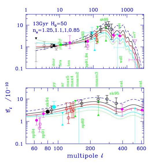
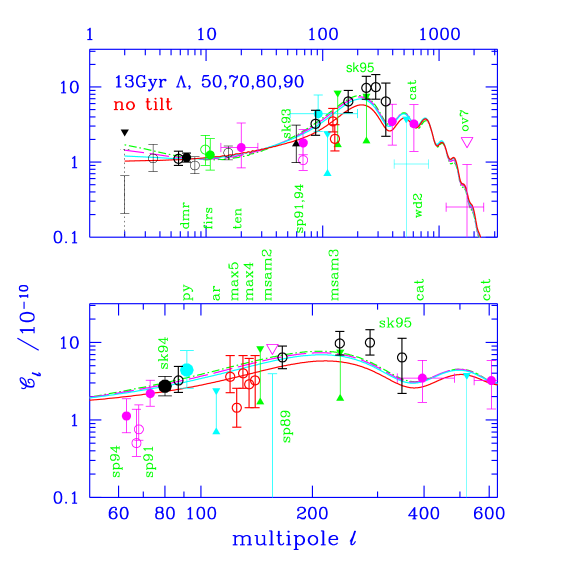
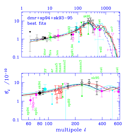
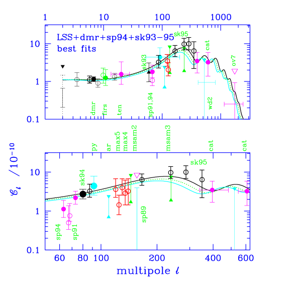
Figure 1: 13 Gyr sequences, varying $n_{s}$ with $\Omega_{vac}=0$, and varying $H_{0}$, hence $\Omega_{vac}$, with $n_{s}=1$.

Figure 2: Best-fit models using DMR+SP94+SK95 on the left, and adding LSS on the right, for 11, 13 and 15 Gyr $\Lambda$ sequences. The left also shows 13 Gyr open and baryon sequence best fits. Parameters defining these models are given in Table 2.

2 Signal-to-Noise Eigenmode Method

We are given the data in the form of a measured mean $\overline{\Delta}_{p}$ of the anisotropy in the $p$th pixel, along with the variance about the mean $\sigma_{Dp}^{2}$ for the measurements. In general, there are pixel–pixel correlations in the noise, defining a correlation matrix $C_{Dpp^{\prime}}$ with off-diagonal components as well as the diagonal $\sigma_{Dp}^{2}=C_{Dpp}$. Also there is usually more than one frequency channel, with the generalized pixels having frequency as well as spatial designations. The theoretical signal also has a correlation matrix, $C_{Tpp^{\prime}}$, which is a linear combination of a product of the ${\cal C}_{{\ell}}$ times a “window function matrix” $W_{pp^{\prime}}(\ell)$ encoding the possibly frequency-dependent beam, the chopping strategy, sky coverage, etc. for the experiment: $C_{Tpp^{\prime}}=\sum_{\ell}{\cal C}_{\ell}W_{pp^{\prime}}(\ell)(\ell+{\textstyle{1\over 2}})/[\ell(\ell+1)]$ (see e.g., [7]). The “window function” usually reported for an experiment is $\overline{W}_{\ell}=(1/N_{pix})\sum_{p=1}^{N_{pix}}W_{pp}(\ell)$.

The likelihood function is

$$\ln{\cal L}(\{y_{A}\})=-\textstyle{1\over 2}\overline{\Delta}^{\dagger}(C_{n}+C_{T})^{-1}\overline{\Delta}-\textstyle{1\over 2}\ln{\rm det}(C_{n}+C_{T})-N_{pix}\ln\sqrt{2\pi}\,.$$ (1)

Here $\dagger$ denotes transpose. The noise correlation matrix $C_{n}=C_{D}+C_{res}$ consists of the pixel errors $C_{D}$ and the correlation of any unwanted residuals $C_{res}$, such as Galactic or extragalactic foregrounds. One can think of $C_{res}$ as increasing the noise for selected correlation patterns in the medium. With a large enough noise in these patterns, they are effectively projected out from the data.

Constraints such as averages, gradients (dipoles, quadrupoles) and known spatial templates, which may be frequency dependent (e.g., IRAS or DIRBE combined with appropriate extrapolations) can also be modelled in the total $\Delta_{p}$, as “nuisance variables” to be integrated (marginalized) over. Denoting each constraint $c$ on pixel $p$ by $\kappa_{c}\Upsilon_{pc}$, where the template for constraint $c$ is $\Upsilon_{pc}$ and the amplitude is $\kappa_{c}$, we need only replace $\overline{\Delta}_{p}$ in eq. (1) by $\overline{\Delta}_{p}-\sum_{c}\Upsilon_{pc}\kappa_{c}$, then integrate over the amplitudes $\kappa_{c}$, assuming some prior probability distribution. This is most easily done if we assume the $\kappa_{c}$ are distributed as very broad Gaussians, reflecting our ignorance of their values (or, if we know their likely range, incorporating that as prior information in the Gaussian spreads). The integration over $\kappa_{c}$ then yields eq.(1) with the residual noise matrix given by $C_{res}=\Upsilon K\Upsilon^{\dagger}$, where $K_{cc^{\prime}}={\langle\kappa_{c}\kappa_{c^{\prime}}\rangle}$ is the assumed prior variance for the constraint amplitudes. As the eigenvalues of $K$ become very large, the effect of the constraint matrix is to project onto the data subspace orthogonal to that spanned by $\Upsilon_{pc}$. Although one can directly use the likelihood equation in this projection limit (using $\delta^{(N_{c})}(\kappa)$ for the constraint prior), it is computationally simpler to use the Gaussian prior. (Taking into account constraints with amplitudes that are not linear multipliers times the template is much more complex.) A suitable $C_{res}$ can also allow us to focus attention only on a specified band in $\ell$-space for power spectrum estimation.

In practice, we do not compute the quantities $\overline{\Delta}^{\dagger}\left(C_{T}+C_{n}\right)^{-1}\overline{\Delta}$ and ${\rm det}[C_{T}+C_{n}]$ directly; instead we go to a basis (i.e., linear combination of the data) in which $C_{T}$ and $C_{n}$ are diagonal. First, we whiten the noise matrix using the nonorthogonal transformation provided by its “Hermitian square root,” $C_{n}\to C_{n}^{-1/2}C_{n}C_{n}^{-1/2}=I$; we apply the same transformation to $C_{T}$ and diagonalize this in turn with the appropriate matrix of eigenvectors, $R$: $C_{T}\to RC_{n}^{-1/2}C_{T}C_{n}^{-1/2}R^{\dagger}={\rm diag}({\cal E}_{k})$, which has units of $(S/N)^{2}$. We then transform the data into the same basis, $\overline{\Delta}\to RC_{D}^{-1/2}\overline{\Delta}=\overline{\xi}$, now in units of $(S/N)$. The transformed theory matrix ${\cal E}$ still depends on the theoretical amplitude ($\sigma_{8}$, etc.) as a simple multiplier, which enables the likelihood to be easily calculated as a function of this parameter. In the new basis, the noise and signal have diagonal correlations and $\langle\xi_{k}^{2}\rangle=1+{\cal E}_{k}$, so $\overline{\xi}_{k}^{2}$ is useful as a theory-dependent $S/N$ power spectrum which gives a valuable picture of the data and shows how well the target theory fares (Fig. 6)[8, 5, 9].

The modes are sorted in order of decreasing $S/N$-eigenvalues, ${\cal E}_{k}$, so low $k$-modes probe the theory in question best. This expansion is a complete (unfiltered) representation of the map. The optimal method for data compression is to use sharp signal-to-noise filtering, keeping only those high $S/N$ modes with $k<k_{cut}$ and deleting low $S/N$ ones. We also find it extremely useful to look carefully at the power in the low $S/N$ modes to determine whether further residuals need to be added to the generalized noise: a poor model for the noise can give false indications of what the data is saying and misrepresent the signal. Filtering using $S/N$-modes has a long history in signal processing where it is called the Karhunen-Loeve method [10], and it is now being widely adopted for analysis of astronomical databases.

For an all-sky experiment with uniform, uncorrelated pixel variances, the eigenmodes are the spherical harmonics, and the eigenvalues the expected coefficients $a_{\ell m}$. For a more complicated experiment, the high-$S/N$ modes probe the peak of the experiment’s window function in $\ell$-space. Low-$S/N$ modes are more complex. For experiments with more than one frequency channel, differences between channels should show no CMB signal, and so the eigenvalue should be $0$. Nearby pixels, oversampling the beam, should also show very little signal—the smooth fall from high $S/N$ to low traces the beam in much the same way that the window function falls as a Gaussian $\propto\exp[-\ell^{2}/\ell_{s}^{2}]$ at high $\ell$. We expect these low $S/N$ modes to be largely independent of the theory used to calculate the appropriate $C_{T}$, which enables these modes to be used as a diagnostic of both the analysis procedure and the experiments themselves.

3 The Experiments Analyzed

We now discuss the anisotropy experiments we use. The six COBE/DMR four-year maps [1] are first compressed into a (A+B)(31+53+90 GHz) weighted-sum map, with the customized Galactic cut advocated by the DMR team, basically at $\pm 20^{\circ}$ but with extra pixels removed in which contaminating Galactic emission is known to be high, and with the dipole and monopole removed. Galactic coordinate pixels are used; slight differences arise with ecliptic coordinate pixels. Although one can do full Bayesian analysis with the map’s $(2.6^{\circ})^{2}$ pixels, this “resolution 6” pixelization of the quadrilateralized sphere is oversampled relative to the COBE beam size, and there is no effective loss of information if we do further data compression by using “resolution 5” pixels, $(5.2^{\circ})^{2}$ [5, 1]. The weighted sum of channels is an exact use of our optimal signal-to-noise compression. The resolution degradation is not optimal but is nearly so ($C_{T}(\theta)$ is nearly constant for separations $\theta$ below the scale of the beam, so adjacent pixel differences have tiny signal but the usual data-noise). The Galactic cut is also not optimal, but could be made so by using explicit templates for Galactic foregrounds to include in $C_{n}$, as described above. The combined effect reduces the pixel number from $6\times 6144$ to $999$. Further compression by a factor of two or so is possible without much information loss [5]. A strong indication of the robustness of the dmr data set is the insensitivity of the band-powers to the degree of signal-to-noise filtering and to which frequencies are probed. For $C_{res}$, we include templates for the monopole, dipole and quadrupole, the latter allowing for a Galactic foreground contaminant, which we know is there at low $\ell$ in the 31 GHz channel. The DMR data probes $\ell\sim 2-15$ well, with useful information out to $\sim 30$.

The sp94 experiment [2] is similar to a classic single-differencing chopping experiment, except that differencing is associated with the oscillation of the beam about the pixel position. It probes $\ell\sim 30-120$. The number of frequency channels and spatial pixels is sufficiently small (301) that no compression is needed: all 7 frequencies in the Ka and Q bands at $\sim 30$ and $\sim 40$ GHz are simultaneously analyzed. There are 14 constraints, average and gradient removals for each frequency. Taking differences in $\Delta T/T$ in frequency at the same spatial position is insensitive to the primary signal but has the usual pixel noise for each channel, so $S/N$ filtering would tend to remove those modes and strong compression would result. Because the beams do vary somewhat with frequency, however, the compression would remove some information, unlike for COBE.

The sk95 experiment [4] probes a much larger band in $\ell$-space, from $\sim 50$ to $\sim 400$. Even before the data was delivered to us a significant amount of frequency and spatial compression already took place. In this paper, for parameter estimation, we use the “CAP” data (2016 pixels, including rebinned data from sk94, with 48 constraints associated with average removals). The SK experiment measured the temperature directly by making slightly-curved radial scans from the North Celestial Pole about 8 degrees in length, which covered the CAP as the earth rotated. The data was binned in RA, but, instead of binning in declination, it was projected in software onto what are in effect 3 to 19 beam “chopping” configurations. Adding the RING data to the CAP, involving sweeps in a ring around the NCP at $\sim 8^{\circ}$ brings the total to 2400 pixels, with 52 constraints. In [9], we show that the “CAP” and “CAP+RING” parameter estimates agree to much better than “one sigma” even though the RING adds substantially more data. One potential concern is that only one HEMT band is represented in the data. We have also extensively analyzed the SK94 data set on its own [3], with 1344 pixels and 28 constraints, which has only 3 to 9 beam template projections and substantially fewer hours of integration than the 94+95 data, but the advantage of having both Ka and Q band information so the frequency spectrum can be checked. We agree with [3] that the spectrum of the SK94 3 to 9 templates is consistent with a CMB origin, and inconsistent with likely Galactic foregrounds. (We come to the same conclusion for the sp94 data, in agreement with [2].) SK95 had data only from the Q-band.

In analyzing SP94 and SK94-95, it is essential to include errors in the overall calibration of $\Delta T$. For SK94-95 it is estimated to be a Gaussian with standard deviation $\varepsilon=0.14$; for SP94, $\varepsilon=0.10$. Let ${\cal L}_{0}(\sigma_{8})$ denote the calculated likelihood assuming no such errors; then the likelihood with the uncertainty included is ${\cal L}(\sigma_{8})=\int d\sigma_{8}^{\prime}\exp[-(\sigma_{8}-\sigma_{8}^{\prime})^{2}/(2\varepsilon^{2}\sigma_{8}^{2})]{\cal L}_{0}(\sigma_{8}^{\prime})$. It is unfortunate that after all of the effort that has gone into these superb experiments, an astronomical issue like the brightness of Cas A (for SK95) results in a substantially poorer constraint on $\sigma_{8}$ than one obtains assuming no such calibration uncertainty.

4 Phenomenology, $S/N$ Power Spectra and Data Compression

As we mentioned in § 1, we have chosen to order our path through parameter-space using the cosmological age of the models, $t_{0}$. To examine the phenomenology of the experiments we shall use a one-parameter sequence of ${\cal C}_{\ell}$ shapes, with the overall bandpower of the experiment (or the related $\sigma_{8}$) as another parameter. While it was usual in the past to use a power law in ${\cal C}_{\ell}$, $\sim(\ell+{\textstyle{1\over 2}})^{\nu_{\Delta T}}$ [8], it is evident from Fig. 2 that this would be a very bad fit to the sk95 data, although it is a reasonable representation over the limited $\ell$ range for both the dmr4 and sp94 data. The sequence we use is the first panel in Fig. 2, the tilted CDM sequence for the standard CDM model, i.e., $H_{0}=50,\Omega=1,\Omega_{B}=0.05$, with $n_{s}$ variable. We use the GW case, i.e., $\nu_{t}=n_{s}-1$ if $n_{s}<1$, $\nu_{t}=0$ otherwise. These models have an age of $t_{0}=13{\rm Gyr}$.

Fig. 4 shows $1,2,3,\ldots$ sigma contours of ${\cal L}(\sigma_{8},n_{s})$, with $\nu$-sigma defined by ${\cal L}/{\cal L}_{max}=\exp[-\nu^{2}/2]$. It is clear from the right hand panel that fixing $n_{s}=1$ and $t_{0}=13$, but varying ${\rm h}$, and therefore $\Omega_{vac}$, is not a good sequence to use for phenomenology since there is very little difference in the ${\cal C}_{\ell}$’s as ${\rm h}$ varies. The Fig. 4 ${\cal L}(\sigma_{8},{\rm h})$ contour map shows that indeed the data does not determine the Hubble parameter very well.

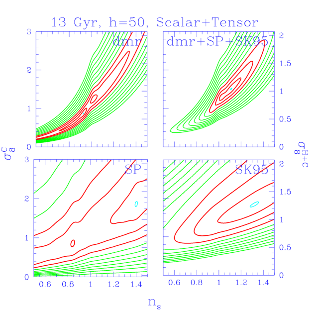
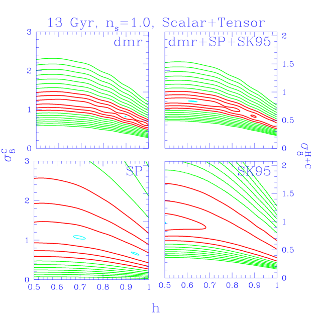
Figure 3: Contour plots of the likelihood of $\sigma_{8}$ and $n_{s}$ for fixed $h=0.5$. The contours are at ${\cal L}$ = $\exp[-{\textstyle{1\over 2}}\{1,4,9,\ldots\}]{\cal L}_{max}$ (with an extra contour around ${\cal L}_{max}$ to show where it is). In every panel, the lefthand $\sigma_{8}$ axis is for the CDM sequence, while the righthand $\sigma_{8}$ axis is for a $\Omega_{hdm}=0.2\Omega_{nr}$ mixed dark matter model. $\sigma_{8}$ inferred from cluster abundances is $\sim 0.6$.

Figure 4: Likelihood of $\sigma_{8}$ and ${\rm h}$ for fixed $n_{s}=1$. In this case, the righthand $\sigma_{8}$ axis strictly applies only for the h=0.5 line.

With the most recent experiments ($N_{pix}\mathrel{\mathchoice{\lower 3.6pt\vbox{\halign{$\mathsurround=0pt\displaystyle\hfil#\hfil$\cr>\crcr\sim\crcr}}}{\lower 3.6pt\vbox{\halign{$\mathsurround=0pt\textstyle\hfil#\hfil$\cr>\crcr\sim\crcr}}}{\lower 3.6pt\vbox{\halign{$\mathsurround=0pt\scriptstyle\hfil#\hfil$\cr>\crcr\sim\crcr}}}{\lower 3.6pt\vbox{\halign{$\mathsurround=0pt\scriptscriptstyle\hfil#\hfil$\cr>\crcr\sim\crcr}}}}2000$), the computer power required to calculate the likelihood over a sufficiently wide model space is becoming prohibitive. The $S/N$-eigenmodes also provide a form of data compression which can drastically reduce the required analysis time. By rotating to a basis in which some “canonical theory” with correlation matrix $C_{T*}$ is diagonalized by the matrix $R_{*}$, but only retaining some fraction of the modes, we efficiently remove parts of the data dominated by noise (i.e., modes with very low $S/N\ll 1$), but retain the Gaussian character of the likelihood for the remaining modes. For other theories, the transformed theory matrix $(R_{*}C_{n}^{-1/2}C_{T}C_{n}^{-1/2}R_{*}^{\dagger})$ will no longer be diagonal, so the full matrix calculation must still be performed, but now on the smaller space of observations restricted to the modes with the highest “canonical” $S/N$. Moreover, for these theories, the $S/N$-modes will be somewhat different, so the compression will not be as efficient (i.e., we will have thrown out a bit “more signal and less noise”). Still, we have achieved compression as good as 90% for experiments (like SK94) with two channels and 65% for the full SK94-95 dataset, which has already been re-binned to remove some of the redundancy in beam oversampling and channel-to-channel differences. Because the cost of the matrix calculations involved scales as $N^{3}$, these result in significant speedups: from $\sim 1$ hour to $\sim 10$ minutes per point in parameter space for sk95 (which is actually significantly worse than the expected $(1-0.65)^{3}\simeq 1/25$ speedup due to overhead).

In Fig. 6, we show $1,2,3,\ldots$ sigma likelihood contours for the SK94-95 CAP dataset, as in Fig. 4. The lower left panel superposes the contours of the $k_{cut}=700$ case upon those with all 2016 modes included. The similarity of the contours shows that both the amplitude and the index determinations are not compromised by $S/N$ cuts. For the $k_{cut}=500$ case, contours $\mathrel{\hbox to0.0pt{\lower 3.0pt\hbox{$-$}\hss}\raise 2.0pt\hbox{$\mathchar 318\relax$}}2$ are very similar as well. Thus we can achieve significant degrees of compression without loss of information. In the following, we apply no data compression to the analysis of the DMR and SP data, but for SK95 we present results using the top 700 modes from the canonical standard CDM theory, the $n_{s}=1$ model in the $t_{0}=13$ Gyr sequence.

The reason the compression works can be understood by examining the $S/N$ power spectra, shown in Fig. 6. The curve is the theoretical spectrum $1+{\cal E}_{k}$ given by the eigenmodes, for a “standard CDM” model with amplitude $\sigma_{8}=1.2$, the value suggested by COBE. The points are the observations $\overline{\xi}_{k}^{2}$, with the same binning as the theory curve. (The bins require a certain signal-to-noise when summed, but a minimum number are required to define a bin so that the error bars are not too large.) The error bars contain both variances associated with the pixel noise and with the theoretical cosmic variance (noise-noise, noise-signal and signal-signal terms). To be a good fit to the data, the error bars should pass through the theory curve. After the top few hundred modes, the eigenvalues have $S/N\ll 1$ so we do not expect them to contribute significantly to the likelihood. We emphasize that it is legitimate to use any mode subset: the relative likelihoods we obtain will tell us which theory is preferred for those modes. It is just that we do not want to build any prior prejudice for a theory by compressing the data in a way which may be biased in its favour over the other theories we are testing. Thus we choose to go far into the $S/N$ tail, retaining 700 modes. The $S/N$ mode formalism also can be used to design experiments to discriminate particular theories (e.g., Knox, these Proceedings).

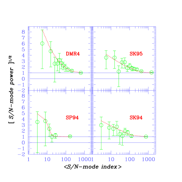
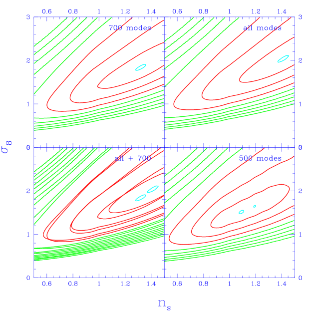
Figure 5: Observed and theoretical $S/N$-spectra with $1\sigma$ errors (including pixel noise and cosmic variance), using “standard” CDM, with $\sigma_{8}=1.2$, the DMR4 value, for the theory.

Figure 6: How $\sigma_{8}$-$n_{s}$ likelihood contours change with the SK95 $S/N$ cut: for 500, 700 and all ($\sim 2000$) modes.

5 Combining Experiments and Parameter Estimation

Combining experiments to get a total likelihood is straightforward. If the pixels are uncorrelated, either because they overlap little on the sky or in $\ell$, we only need to multiply the individual likelihoods together. This is the case for COBE/DMR, SP94, SK94-95. If there is significant overlap, then the experiments should ideally be combined and considered to be one larger experiment, with $C_{T}$ connecting the pixels in one experiment with the pixels in the other, although the cross-pixel $C_{D}$ will be zero. We have applied this to the SK95+MSAM dataset, in joint work with Charbonneau and Knox, but will not describe it here.

The upper right panel of Fig. 4 shows the likelihood for the $H_{0}=50$, GW, 13 Gyr, tilted sequence. Each experiment individually constrains the amplitude, $\sigma_{8}$, better than the shape, $n_{s}$: the window functions cover a narrow range of $\ell$. Note that the SK experiment does better than DMR at determining the slope. The calibration uncertainty for SK95 is the reason that $\sigma_{8}$ is not more tightly constrained. Fig. 4 shows the advantage offered by combining the results of different experiments: the long baseline in $\ell$ helps considerably in localizing the $n_{s}$ contours. In Fig. 4, we see that the DMR data does not restrict the value of ${\rm h}$, and thus not of $\Omega_{vac}$, whereas the SK data does, yet the combined data focusses the $\sigma_{8}$ determination, but not the ${\rm h}$ determination. The SK95 data prefers more power than is predicted by the DMR data for “standard” models. Thus, the $n_{s}=1$, $H_{0}=50$, $\Omega_{B}{\rm h}^{2}=0.0125$ model has $\sigma_{8}=1.20\pm 0.08$ for DMR, while for SK95 it is $\sigma_{8}=1.48^{+0.26}_{-0.20}$. Increasing $\Omega_{B}{\rm h}^{2}$ to 0.2 brings them closer into line, $\sigma_{8}=0.89\pm 0.06$ for DMR, while for SK95 it is $\sigma_{8}=0.82^{+0.15}_{-0.11}$; and this model is much preferred statistically to the 0.0125 one.

We could repeat the contour maps for the 11 and 15 Gyr vacuum sequences, for the fixed $t_{0}$ open models, and for the variable $\Omega_{B}$ sequence, but it is more concise to quote single numbers, our estimates of the individual cosmological parameters. To that end, we marginalize over the other parameters in the sequence, assuming a prior probability for the parameters. If it is uniform we get the results in the left columns of Table 1. The idea that first motivated this project was that the SK94 and SP94 data looked sufficiently robust to return to the multiresolution approach combining experiments to get best possible constraints, e.g., [7], and this would significantly improve the COBE-only errors on $n_{s}$. The SK94+SP94+DMR4 column is the culmination of that effort. However, the SK95 data took us to significantly higher $\ell$ and the promise of greater discrimination among models based on how they rise to the Doppler peak. Notice the rather large shift in $n_{s}$ when we pass from the 1300 pixel 2-channel SK94 data, which had chopping templates from 3 to 9, to the SK95 set, which had 10-19 projections as well as much more 3-9 data, but only for the Q-band. A worry is that non-cosmic signals at high $\ell$ might be contaminating the 10-19 template projections.

case		DMR4	SK94+SP94	SK94-95	LSS+DMR4	LSS+DMR4
			+DMR4	+SP94+DMR4		+SK94-95+SP94
13 Gyr $\Omega_{vac}$ sequence, with GW
$H_{0}$=50	$n_{s}$	$1.02^{+.23}_{-.18}$	$0.95^{+.05}_{-.08}$	$1.12^{+.11}_{-.09}$	$0.76^{+.03}_{-.03}$	$0.85^{+.02}_{-.02}$
$H_{0}$=70	$n_{s}$	$1.12^{+.26}_{-.24}$	$0.92^{+.05}_{-.05}$	$1.12^{+.09}_{-.12}$	$0.99^{+.03}_{-.02}$	$0.99^{+.03}_{-.02}$
All $H_{0}$	$n_{s}$			$1.11^{+.11}_{-.10}$	$1.02^{+.40}_{-.06}$	$1.07^{+.13}_{-.08}$
$n_{s}$=1	$H_{0}$	$<90$	$<65$	$<65$	$68\pm 3$	$67\pm 3$ ($\Omega_{vac}\approx 0.60$)
All $n_{s}$	$H_{0}$			$<76$	$<68$	$70\pm 4$ ($\Omega_{vac}\approx 0.66$)
15 Gyr $\Omega_{vac}$ sequence, with GW
$H_{0}$=43	$n_{s}$	$1.02^{+.22}_{-.18}$	$0.93^{+.05}_{-.06}$	$1.04^{+.13}_{-.06}$	$0.84^{+.03}_{-.03}$	$0.91^{+.03}_{-.04}$
$H_{0}$=70	$n_{s}$	$1.28^{+.21}_{-.33}$	$0.89^{+.08}_{-.08}$	$1.02^{+.16}_{-.06}$	$1.25^{+.04}_{-.04}$	$1.26^{+.03}_{-.04}$
All $H_{0}$	$n_{s}$			$1.05^{+.12}_{-.08}$	$1.17^{+.15}_{-.18}$	$1.03^{+.14}_{-.04}$
$n_{s}$=1	$H_{0}$	$<76$	$<51$	$<61$	$54\pm 3$	$53\pm 2$ ($\Omega_{vac}\approx 0.50$)
All $n_{s}$	$H_{0}$			$<63$	$<57$	$55\pm 4$ ($\Omega_{vac}\approx 0.52$)

Table 1: Some results for $n_{s}$ and $H_{0}$ from our analysis for various combinations of experiments as indicated. Upper limits and error-bars are “1-$\sigma$” ones determined using likelihood ratios ${\cal L}=e^{-1/2}{\cal L}_{max}$. In rows 1, 2 and 4 for each case, $H_{0}$ or $n_{s}$ is fixed and only $\sigma_{8}$ is marginalized. The other two marginalize over $H_{0}$ or $n_{s}$ as well as $\sigma_{8}$. In all cases, we have fixed $t_{0}=13$ Gyr, $\Omega_{B}{\rm h}^{2}=0.0125$, $\Omega_{tot}=1$ and included tensor modes for $n_{s}<1$. Note that whether the small angle experiments are added to LSS+DMR4 or not has little impact on the $n_{s}$ ($H_{0}$) estimation if $H_{0}$ ($n_{s}$) is fixed.

DMR4+SP94+SK94-95 BEST FIT MODELS, with GW
case	$H_{0}$	$n_{s}$	$\Omega_{vac}$	$\sigma_{8}$
13 Gyr $B$	50	$1.15$	0	$1.8$ (1.24)	($\Omega_{B}=0.013$)
13 Gyr $B$	50	$1.0{\bf F}$	0	$0.9$ (0.62)	($\Omega_{B}=0.17$)
15 Gyr $\Lambda$	43	$1.05$	0	$1.1$ (0.76)	($\Omega_{B}=0.068$)
13 Gyr $\Lambda$	50	$1.15$	0	$1.3$ (0.90)	($\Omega_{B}=0.05$)
13 Gyr $\Lambda$	60	$1.0{\bf F}$	0.43	$1.22$	($\Omega_{B}=0.035$)
11 Gyr $\Lambda$	59	$1.2$	0	$2.2$ (1.54)	($\Omega_{B}=0.036$)
13 Gyr OPEN	55	$1.05$	$\Omega_{tot}$=0.60	1.0	($\Omega_{B}=0.041$)
LSS + DMR4+SP94+SK94-95 BEST FIT MODELS, with GW
15 Gyr $\Lambda$	55	$1.0$	0.52	$0.97$	(best fit)
13 Gyr $\Lambda$	65	$1.0$	0.56	$1.17$	($1\sigma$ down)
11 Gyr $\Lambda$	85	$1.05$	0.69	$1.49$	($2\sigma$ down)

Table 2: “Best fit” models for various regions in the scanned parameter space. The top panel considers the combined likelihoods from the CMB experiments. In the $\sigma_{8}$ column, the numbers in parentheses are the equivalent values for a cold+hot dark matter universe with $\Omega_{hdm}=0.2$. For the $\Lambda$ cases, $\Omega_{B}$ is not varied separately, but fixed at $\Omega_{B}{\rm h}^{2}=0.125$. The bottom panel adds in the prior information from large-scale structure and lists the best fit model for each age, as well as their relative likelihoods. ${\bf F}$ means the parameter value was forced to be the one indicated.

We now wish to add some large scale structure constraints, by constructing prior probabilities that roughly correspond to the restrictions arising from observations of galaxy clustering and cluster abundances. The linear power spectrum for density fluctuations is often characterized by the shape parameter, $\Gamma\approx\Omega_{nr}{\rm h}\,e^{-[\Omega_{B}(1+\Omega_{nr}^{-1}(2{\rm h})^{1/2})-0.06]}$, which is 0.48 for the standard CDM model. Here $\Omega_{nr}=\Omega_{B}+\Omega_{cdm}+\Omega_{hdm}$. Assuming a linear bias model for how the galaxy distribution is amplified over the mass distribution, the clustering data implies $0.15\mathrel{\hbox to0.0pt{\lower 3.0pt\hbox{$\mathchar 536\relax$}\hss}\raise 2.0pt\hbox{$\mathchar 316\relax$}}\Gamma+\nu_{s}/2\mathrel{\hbox to0.0pt{\lower 3.0pt\hbox{$\mathchar 536\relax$}\hss}\raise 2.0pt\hbox{$\mathchar 316\relax$}}0.3$. The abundance as a function of X-ray temperature also heavily constrains $\sigma_{8}$. Values from 0.5 up to 0.7 are obtained for $\Omega_{nr}=1$ CDM-like models. For $\Omega_{vac}>0$, the value is higher, scaling roughly as $\Omega_{nr}^{-0.56}$. There are also many estimates of the combination $\sigma_{8}\Omega_{nr}^{0.56}$ that are obtained by relating the galaxy flow field to the galaxy density field inferred from redshift surveys, which all take the form $[b_{g}\sigma_{8}]\,\beta_{g}$, where $b_{g}$ is the galaxy biasing factor and $\beta_{g}$ is a number whose value depends upon data set and analysis procedure: [11] give $0.64\pm 0.27$ for an average of a number of estimates in the literature, and $0.55\pm 0.10$ for a determination using a maximum likelihood technique for the IRAS survey and the Mark III velocity field data set, while a higher ($\sim 0.7$) number is obtained using POTENT on this data set. It is usual to take $b_{g}\approx\sigma_{8}^{-1}$ for galaxies, which gives a $\sigma_{8}$ consistent with the cluster value, but $b_{g}$ can depend upon the galaxy types being probed, upon scale, and could be bigger or smaller than $\sigma_{8}^{-1}$.

We want to choose priors for $\sigma_{8}$, $\Omega_{vac}$ and $\nu_{s}$ that reflect these LSS ranges, but we certainly don’t want to be too miserly in our choice of allowed ranges. A straight Gaussian tends to be overly supportive of the mean, while a tophat error has no probability in the wings. Using priors which convolve a Gaussian with a tophat and have different upper and lower errors give us the flexibility we require. It is similar to specifying both a statistical and a systematic error. For the exercise shown in the tables, we required that $\Gamma+\nu_{s}/2$ be $0.22^{+0.07+0.08}_{-0.04-0.07}$ and $\sigma_{8}\Omega_{nr}^{0.56}$ be $0.65^{+0.02+0.15}_{-0.02-0.08}$. The latter has a high probability at 0.55, but little at 0.50 (although some authors actually prefer this value). Sample LSS+CMB numbers are given in Table 1.

The tiny error bars when LSS constraints are added to the CMB data are amusing, but are far from definitive at this stage. The reason the errors are small is typically that the CMB data pushes for a likelihood peaked at high $\sigma_{8}\mathrel{\hbox to0.0pt{\lower 3.0pt\hbox{$\mathchar 536\relax$}\hss}\raise 2.0pt\hbox{$\mathchar 318\relax$}}1$, and this multiplies the LSS likelihood peaking at 0.6 or so. The product of the two has a narrow peak but also a small likelihood. This asymmetry is not as pronounced for the hot/cold hybrid models.

Table 2 gives the parameters for the best fits to the data for the various cases. The associated ${\cal C}_{\ell}$’s are shown in Fig. 2. Note that the models which best fit the CMB data for a given age often have positive tilts. While positive scalar tilt is possible in inflation models, it requires special constructs in the inflaton potential in a region corresponding to just where we can observe it with the CMB. More likely are negative tilts. If we restrict our attention to these (e.g., second row), then the best fit for the $\Omega_{B}$ sequence (13 Gyr, $H_{0}=50$) is $n_{s}\approx 1$ and $\Omega_{B}\approx 0.17$, high not low. In the lower LSS part of Table 2, the 13 Gyr best fit is one sigma down from the 15 Gyr best fit, and the 11 Gyr is two sigma down.

The analysis shows that $n_{s}$ lies close to the value predicted by inflation. The $H_{0}$ limits are suggestive, but better CMB data is needed to strengthen the constraint to usable values. Of course when the LSS data are included, $\Omega_{vac}>0$ is suggested for $n_{s}=1$ CDM models, though it is not needed for hot/cold hybrids with $\Omega_{hdm}=0.2\Omega_{nr}$. Table 1 shows adding SK95 and SP94 to LSS and DMR4 does not add much further discrimination, but this should change dramatically in the next few years, with the advent of long duration balloon experiments, interferometers, MAP and COBRAS/SAMBA.

We would like to thank Barth Netterfield and Lyman Page for helping us understand how to model their data and Lloyd Knox for useful conversations.

References

- [1] C. Bennett et al. , 1996, Ap. J. Lett.464, L1; and 4-year DMR references therein.
- [2] J.O. Gundersen et al. , 1995, Ap. J. Lett., 443, L57 sp94.
- [3] C.B. Netterfield, N. Jarosik, L. Page & D. Wilkinson, 1995, Ap. J. Lett. 455, L69. sk94.
- [4] C.B. Netterfield, M.J. Devlin, N. Jarosik, L. Page & E.J. Wollack, 1996, Ap. J., submitted sk95.
- [5] J.R. Bond, 1994, Phys. Rev. Lett. 74, 4369.
- [6] B. Chaboyer et al. , 1996, Science, in press.
- [7] Bond, J.R. 1996, Theory and Observations of the Cosmic Background Radiation, in “Cosmology and Large Scale Structure”, Les Houches Session LX, August 1993, ed. R. Schaeffer, Elsevier Science Press.
- [8] J.R. Bond, 1995, Astrophys. Lett. & Comm., 32, 63.
- [9] Bond, J.R. & Jaffe, A., 1996, CITA preprint.
- [10] C.W. Therrien 1992, Discrete Random Signals in Statistical Signal Processing, ISPN0-13-852112-3 (Prentice Hall).
- [11] M. Strauss, & J. Willick, J. 1995, Phys. Rep. 261, 271