Filament and Shape Statistics: A Quantitative Comparison of Cold + Hot and Cold Dark Matter Cosmologies vs. CfA1 Data

Abstract

A new class of geometric statistics for analyzing galaxy catalogs is presented. Filament statistics quantify filamentarity and planarity in large scale structure in a manner consistent with catalog visualizations. These statistics are based on sequences of spatial links which follow local high-density structures. From these link sequences we compute the discrete curvature, planarity, and torsion. Filament statistics are applied to CDM and CHDM ($\Omega_{\nu}=0.3$) simulations of Klypin et al. (1996), the CfA1-like mock redshift catalogs of Nolthenius, Klypin and Primack (1994, 1996), and the CfA1 catalog. We also apply the moment-based shape statistics developed by Babul & Starkman (1992), Luo & Vishniac (1995), and Robinson & Albrecht (1996) to these same catalogs, and compare their robustness and discriminatory power versus filament statistics. For 100 Mpc periodic simulation boxes ($H_{0}=50$ km s^-1 Mpc^-1), we find discrimination of $\sim 4\sigma$ (where $\sigma$ represents resampling errors) between CHDM and CDM for selected filament statistics and shape statistics, including variations in the galaxy identification scheme. Comparing the CfA1 data versus the models does not yield a conclusively favored model; no model is excluded at more than a $\sim 2\sigma$ level for any statistic, not including cosmic variance which could further degrade the discriminatory power. We find that CfA1 discriminates between models poorly mainly due to its sparseness and small number of galaxies, not due to redshift distortion, magnitude limiting, or geometrical effects. We anticipate that the proliferation of large redshift surveys and simulations will enable the statistics presented here to provide robust discrimination between large-scale structure in various cosmological models.

1 Introduction

In this paper we develop and apply statistics to quantitatively characterize the shapes of galaxy distributions seen in redshift surveys. We then use these statistics to compare cosmological simulations of pure Cold Dark Matter (CDM) models versus Cold plus Hot Dark Matter (CHDM) models in real space, as well as simulated CfA1-like redshift surveys generated from these simulations versus the CfA1 data. The four simulations used here are summarized in Table 1 and described in detail in §4.1. The availability of this suite of simulations of different cosmological models, all computed and analyzed in parallel, allows us to test the ability of these statistics to discriminate between such models. Visual comparison of the simulations (Brodbeck et al. 1996; hereafter BHNPK) shows that the CDM galaxy distribution contains larger clusters and less well-defined filamentary and sheet-like structures than CHDM, consistent with the fact that CHDM forms structure at a later epoch than CDM. The statistics presented here confirm as well as quantify these results, showing statistically significant and robust discrimination between the models.

Ever since the CfA1 Survey (deLapperant, Geller & Huchra 1988) detected filamentary and planar structures in the galaxy distribution, many attempts have been made to develop statistics computed solely from the redshift-space positions of galaxies which quantify these large-scale structures. It became apparent that the two-point correlation function contains very limited information about structure, while higher-order correlation functions are difficult to measure and mainly decribe the highest density regions. Thus alternative, more geometrical methods have been developed which contain information from all orders of correlation functions in such a way as to characterize the types of structures seen in the surveys. The void probability function (e.g. Vogeley, Geller & Huchra 1991, Ghigna et al. 1994, 1996) and the topological genus statistic (see Melott 1990 for review, and Coles, Davies & Russell 1996 for related discussion) have had some success, and lately more complex statistics have been developed which seem promising such as the Minkowski Functionals (Mecke, Buchert & Wagner 1994 and Kerscher et al. 1996).

Here we introduce filament statistics, a new class of geometric statistics designed to quantify filamentarity and planarity in large-scale structure. Filament statistics use information about the moments of the local mass distribution to characterize the shape of large-scale structure. In this way they are similar to the shape statistics of Babul & Starkman (1992; hereafter BS), Luo & Vishniac (1995; hereafter LV), and Robinson & Albrecht (1996; hereafter RA). However, the way in which the moment tensor information is used in filament statistics is fundamentally different from these shape statistics. Rather than randomly sampling the galaxy distribution, filament statistics use a prescription to map the galaxy distribution into a new set of points which amplifies the properties showing the greatest differences between models, namely filamentarity and planarity. While statistics applied to the new point set can be more discriminatory, care must be taken to develop a prescription which is robust against inherent variations in the simulated galaxy distribution such as galaxy identification uncertainty and cosmic variance. Hence in constructing filament statistics, we are guided by the following principles:

• It is best to attempt to directly quantify structures which visually show the greatest differences between models, i.e. filaments and sheets.

• It is best to apply statistics directly to the point set of galaxies rather than a smoothed density distribution to avoid discarding information on small scales.

• It is best to construct simple, interpretable statistics, in order to more easily understand their robustness against intrinsic uncertainties in the analysis.

We find that both our filament statistics and the BS, LV and RA shape statistics yield statistically significant discrimination between CDM and CHDM simulations, which persists (though to a significantly lesser degree) even in a redshift-space comparison versus the CfA1 data. A more informative comparison of these statistics must await the availability of larger, more complete redshift surveys as well as simulations capable of properly modeling these large volumes of space; both should be available soon. For now, we present these results to demonstrate the viability of the methods. We note that this is the first publication in which any of these moment-based shape statistics have been used to compare simulations to redshift survey data, which is the purpose for which they were originally devised.

2 Implementation of Filament Statistics

2.1 Dekel’s Alignment Statistic

Our filament statistics are related to the alignment statistic, originally proposed by Dekel (1984): For each galaxy, consider two concentric shells; find the moment of inertia ellipsoid axes defined by galaxies within each shell; and calculate the angle difference between the inertia tensor axes. Presumably, where the angle difference in the major axis is small, there is a filamentary structure present, and where the angle difference in the minor axis is small, there is a sheet-like structure present. By randomly sampling the galaxy distribution at different shell radii, one can then gain a measure of the filamentarity and planarity in large-scale structure at various scale lengths. However, we found that the alignment statistic barely discriminated between CDM and CHDM in real 3D space, and failed to discriminate the models in redshift space.

Since the visualizations of BHNPK show marked differences in the number, size, and continuity of filamentary structures in CHDM and CDM, we were inspired to consider mapping the point set of galaxies into another point set by an algorithm that sensitively favors contiguous high density regions.

2.2 The Creation of Link Sequences

The basis of filament statistics is the creation of link sequences which follow along local high density regions, as determined by the principal axis of the local moment of inertia tensor. Link sequences may be thought of as a technique to map the point set of galaxies into a new point set which emphasizes the higher density regions containing the filamentary and planar structures which we would like to quantify. A statistic applied to this new point set is likely to be more discriminatory than the same statistic applied to a random subset of galaxies; this is the case with the alignment statistic. Most other statistics presented in the literature (including BS, LV, and RA statistics) use sampling of the data points to obtain a measure of the global structure; filament statistics represents a new method for manipulating the data to enhance the structures of interest, thereby enhancing the discriminatory power of a given statistic.

A link sequence is an ordered set of points which can be visualized as joined by “links”, created by the procedure outlined in the flowchart in Figure 1. A link sequence is started from each galaxy in a catalog of galaxies (or if there are too many, a random subset of such galaxies). The moment of inertia tensor is computed using the masses and positions of galaxies within a range $R$ of the given point; for redshift survey data, we weight by luminosity instead of mass. The eigenvectors and eigenvalues of the inertia tensor are found, and from these the principal axis is determined. The new point in the sequence is created at a distance $L$ (the “link length”) away in the direction of the principal axis, and a link is created which joins the old point to the new point. Note that only the first point in a link sequence is a galaxy; the others are simply locations within the catalog volume. A new inertia tensor is computed around this new point, and the procedure is repeated until termination. Sequence termination occurs when there are too few nearby galaxies to reasonably identify an axis. By this prescription, each galaxy generates a sequence of links. If a sequence has more than $N_{L,min}$ links, then statistics are computed on this link sequence, otherwise the sequence is discarded. The construction of a link sequence is completely defined by choosing the link length $L$, the maximum radius of galaxies to be included in computation of the moment tensor $R$, and the criteria for termination of a sequence.

Note that the principal axis of the inertia tensor does not define a unique direction. So from the initial point, the sequence is propagated in both (opposing) directions until termination, and the entire joined sequence is what is used for statistical analysis, as long as the total number of links is at least $N_{L,min}$. Generally, sequences tended to be non-intersecting but in some cases they oscillated between two points. When this is detected, the sequence is terminated.

2.3 Constructing a Dimensionless Statistic

We would like to construct dimensionless parameters which describe the shapes of structures. For that we need to express all scales in units of some typical length scale of the catalog. A natural choice is the mean intergalaxy spacing $\bar{d}\equiv(V/N)^{1/3}$, where $V$ is catalog volume and $N$ is number of galaxies in the catalog, since it provides a length scale independent of galaxy clustering; it is also the simplest choice.

We will consider applications in real space as well as magnitude-limited and volume-limited redshift space. Redshift distortion will produce measurable effects on link sequences, and attempts will be made to understand and quantify these effects. Whereas in real space the mapping of a galaxy into a link sequence is completely well-defined, in redshift space this is no longer true — redshift distortion for a given structure depends on the vantage point chosen to observe the structure. In this paper we introduce a new method for quantifying how redshift-space distortion affects these statistics. We show that none of the statistics analyzed here are adversely affected by redshift distortion to any significant degree.

A complication arises in computing $\bar{d}$ in magnitude-limited catalogs, since the sample incompleteness increases with distance from the Milky Way origin, making $\bar{d}$ a function of radius from origin. A local computation of $\bar{d}$ around a given sequence point (i.e., using $\bar{d}=(V/N)^{1/3}$ for a local volume $V$ around the given point) will degrade the statistics, since structure identification will be biased towards underdense regions where $\bar{d}$ is large, which is exactly opposite of what is desired. Instead, $\bar{d}$ should be corrected using the selection function, which depends only on the distance $r$ from the origin. Since $\phi(L)dL$ is the number density of galaxies between luminosity $L$ and $L+dL$, we can obtain $\bar{d}(r)$ for galaxies visible above the magnitude limit as follows:

$$\bar{d}(r)=\left[{\int^{\infty}_{L_{\em lim}(r)}\phi(L)dL}\right]^{-1/3}$$ (1)

where $L_{\em lim}(r)$ is the luminosity of a galaxy with apparent magnitude 14.5 (the CfA1 magnitude limit) at a distance $r$. $\phi(L)$ is assumed to have Schecter form

$$\phi(L)dL=\phi^{\ast}\biggl{(}{L\over L^{\ast}}\biggr{)}^{\alpha}\exp(-L/L^{\ast}){dL\over L^{\ast}}$$ (2)

The Schecter parameters $\phi^{\ast}$, $L^{\ast}$ and $\alpha$ were best-fit to each real and simulated redshift catalog individually; this procedure is described in Nolthenius et al. (1994, 1996; NKP94 and NKP96, respectively). Note that the true distance $r$ is unknown, and is instead estimated assuming no peculiar velocities, i.e. $r\equiv v/H_{0}$ for a galaxy with radial velocity $v$. In the CfA1 data, a few blueshifted galaxies (mostly in Virgo) do end up on the opposite side of the origin, but the statistics turn out to be insensitive to where these few galaxies are placed. ${\bar{d}(r)}$ is computed and used as the local mean intergalactic spacing at each sequence point in the analysis of magnitude-limited catalogs.

2.4 Link Parameters

The first parameter choice we tried was the simplest, with $L=R=\bar{d}$. The virtue of this definition is that we have a parameter-free statistic, in the sense that the parameters are all determined from intrinsic properties of the data set. Unfortunately, statistics derived from constructions with these “natural” parameters did not discriminate between models. $R=\bar{d}$ turns out to be too small to identify a local structure, and is dominated by shot noise.

For link length $L=\bar{d}$, but range $R$ left as a free parameter, we obtain discriminatory statistics; this choice of $L$ appears to work as well as any other. However, for $R=\bar{d}$, and $L$ a free parameter, we again find little discrimination between models, or even from a Poisson catalog. A larger $R$ will yield more points per sphere, thereby lowering shot-noise scatter. Since the $R$ parameter controls the scales of structure being measured by the statistics, it is interesting and instructive to look at statistics as a function of $R$, and the results will be presented that way.

2.5 Termination Criteria

There are three parameters which set the termination criteria for a link sequence. $N_{P,min}$ is the minimum number of galaxies required within a sphere of radius $R$ for a sequence to continue; $N_{P,min}$ was set to 5 so that the determination of the principal axis would be statistically meaningful, and so that a sequence would terminate if it was in a sparse region in the catalog. $N_{L,max}$ sets the maximum number of links for a periodic catalog, and is set so that the total length of a sequence cannot exceed the length of the simulation box. In a redshift survey, the sequence terminates if it exceeds the catalog boundary. $N_{L,min}$ sets the minimum number of links for a sequence to be statistically meaningful. This was set to 4 links (the minimum value for computation of all statistics), but can be increased to explore more extended structures. However, since each link is typically fairly large ($\approx$3 Mpc in the simulations considered, and $\approx$15 Mpc in the sparser CfA1 catalog), 4 links is already exploring a reasonably extended scale.

All the termination parameters were varied over fairly wide ranges. $N_{P,min}$ was varied from 4 to 10 with little change in discrimination or robustness; any higher, and the shot noise generated from fewer sequences became significant. The statistics are independent of $N_{L,max}$ as long it is above about 10, below which shot noise from the small number of links becomes significant; it is $\sim 34$ in the periodic simulation boxes. Variations in $N_{L,min}$ had some effect on the results for real and simulated redshift catalogs, since for very small values (2 or 3) shot noise increases from low link sampling, while for a high value (above 10), the number of acceptable sequences decreases so that catalog sampling shot noise becomes large. Discrimination was also insensitive to the choice of either a Gaussian, exponential, or top hat window function; we used a top hat for computational efficiency.

2.6 Computation of Statistics

Once link sequences have been generated, there are two ways the new point set may be used. We may choose to apply statistics which were previously applied to random subsets of the data to this new point set. Alternatively, we may devise statistics which measure the properties of link sequences themselves. Filament statistics are based on the latter idea, following the intuitive characterizations of structure given by the alignment statistic.

We developed three statistics to compute on a link sequence which measure filamentarity or planarity in an easily interpretable way. We call them planarity, curvature, and torsion. These statistics are in general defined as angle deviations between inertia ellipsoid axes for consecutive points along a link sequence; the exact definitions are as follows:

• Planarity ($\theta_{P}$) is the angle difference between the minor axis of the inertia tensor for two consecutive points. The geometrical interpretation of planarity is as follows: Given that filaments in large-scale structure often occur at intersections of sheet-like structures, the minor axis of the inertia tensor along the filament measures the strength of the embedding sheet perpendicular to the filament; hence a lower planarity angle indicates the presence of a local sheet-like structure.

• Curvature ($\theta_{C}$) is defined as the angle difference between two consecutive links. Equivalently, it is the angle difference between the major axis of the inertia tensor for two consecutive points. A sequence which is following a well-defined filament will have a low angle difference between links; hence a lower curvature angle indicates greater filamentarity.

• Torsion ($\theta_{T}$) is the angle difference between the plane defined by the first two links and the third link. Torsion measures the strength of the embedding sheet parallel to the filament, a lower torsion indicating a stronger planar structure present.

In all cases, a lower value (angle difference) signifies more structure present in the catalog. As an example, consider a set of points distributed randomly throughout a long, thin cylinder. A sequence will track the cylinder, and the angle deviation between each successive link will be very small; hence curvature will show a very low angle deviation. Conversely, planarity and torsion will show large angle deviations since there is no locally preferred plane in a circular cylinder. For a thin sheet, sequences will randomly walk throughout the sheet, yielding a high curvature angle (indicating no filamentary structure), but low planarity and torsion angles (indicating lots of planar structure).

In large-scale structure, filaments are often embedded within sheets, and thus these statistics are expected to be correlated. Nevertheless it is useful to consider each one separately. A key difference between the statistics is that each requires a different number of sequence points to compute. Planarity is the most local statistic, being computed from only 2 link nodes, while curvature requires 3, and torsion requires 4. While planarity and torsion are in the ideal case purely measures of planarity, torsion is more sensitive to the presence of local filamentary structure since it measures angle differences along the sequence rather than perpendicular to the sequence.

For each of those statistics, an average value is found within a single sequence. Then, for all the sequences in that catalog, a median value is found. We will denote the resulting averaged-then-medianed statistic by a bar, as in $\bar{\theta}_{C}$. This final median value is the value of that statistic for the given catalog at the selected value of $R$. Errors analysis is discussed in section 4.

2.7 Visualization and Algorithm Testing

We have attempted to construct an algorithm which will identify and track filaments. We tested the algorithm on artificially generated point sets of lines and planes of varying thickness. The results conformed to qualitative expectations, that lines should show a great deal of filamentarity and little planarity, and vice versa for planes. Also, the median angle deviations increased with thickness, as expected. Visualizations showed that link sequences were tracking the structure as expected.

When we visualized the link sequences which were generated in an actual CHDM simulation, they tended to lie preferentially in regions of structure, but could not often be associated with visually recognizable filaments. They were also scattered throughout the simulation volume. This is because for the simulations we considered (which will be described in the next section), nearly every galaxy that was tried as a sequence starting point yielded a qualifying ($N_{L,min}\geq 4$) sequence. Thus the parameter set we have chosen does not sufficiently restrict the generated sequences to lie directly along the filaments that are detected by eye. By imposing more severe requirements for sequence qualification, one can tune the algorithm to better recognize filamentary patterns. However, this reduces the number of qualifying sequences to a point where statistics are poor, and hence it is not useful for performing statistically significant comparisons. Our conclusion is that this algorithm is not particularly suited for pattern recognition, and is better suited for statistical comparison of overall structural properties of models. The statistics we compute have simple interpretations, and the results for various models are consistent with the BHNPK visualizations; however, this agreement is not necessarily apparent from visualizations of individual link sequences.

Little effort went into developing analytical predictions for expected values of $\bar{\theta}_{C}$, $\bar{\theta}_{P}$, and $\bar{\theta}_{T}$, even in the case of a Poisson catalog. This is due primarily to the fact that the algorithm was successful in the test cases we considered, and thus a complex and time-consuming analytical prediction was deemed to be low priority. Further numerical testing may also be done by superimposing lines or sheets of varying strengths on a Poisson catalog, and determining how effective the algorithm identifies structure. We leave these endeavors to the future, and instead for now concentrate on applications to the comparison of cosmological models.

3 Moment-Based Shape Statistics

As a brief review, we present the definitions of statistics given by BS, LV, and RA. Since one of the authors independently derived the LV statistics (Hellinger 1995), we present those first and in somewhat more detail. The construction of each family of statistics is well-motivated and elegantly presented in the relevant papers; we refer the reader to them for further details, and here focus on the definitions.

3.1 Luo & Vishniac Shape Statistics

The statistics presented in LV are a three-dimensional extension of the two-dimensional shape statistics devised by Vishniac (1986). In three dimensions, LV statistics are given by a linear combination of the quadratic coordinate moment invariants (summations implied by repeated indices):

$$LV = C_{1}({\cal M}^{ii})^{2}+C_{2}({\cal M}^{ij})^{2}+C_{3}({\cal M}^{ii})({\cal M}^{j})^{2}$$ (3)

$$-C_{4}({\cal M}^{ij})({\cal M}^{i})({\cal M}^{j}),$$

where

$${\cal M}^{i} \equiv {1\over M}\sum_{k}m_{k}(x_{k}^{i}-x_{0}^{i})$$

$${\cal M}^{ij} \equiv {1\over M}\sum_{k}m_{k}(x_{k}^{i}-x_{0}^{i})(x_{k}^{j}-x_{0}^{j})$$

$$M \equiv \sum_{k}m_{k}$$ (4)

are summed over all galaxies at ${\bf x}_{k}$ with masses $m_{k}$ within a window radius $R$ of a central galaxy at ${\bf x}_{0}$. The constants $C_{i}$ are determined by the constraints applicable for a given shape. For a “filamentarity” statistic we have

$$\left\{\begin{array}[]{ll}LV\equiv 0\mbox{ for a spherical distribution entirely within}\;R\\ LV\equiv 0\mbox{ for a distribution with a uniform gradient,}\\ \;\;\;\;\mbox{of arbitrary size, in the window defined by}\;R\\ LV=1\mbox{ for a uniform linear density passing }\\ \;\;\;\;\mbox{through the window center}\end{array}\right.$$

This yields the quadratic filamentarity statistic:

$$LV_{\sl quad} = \frac{1}{({{\cal M}}^{ii})^{2}}\{-\frac{1}{2}({\cal M}^{ii})^{2}+\frac{3}{2}({\cal M}^{ij})^{2}$$ (5)

$$+\frac{1}{2}({\cal M}^{ii})({\cal M}^{j})^{2}-\frac{3}{2}({\cal M}^{ij})({\cal M}^{i})({\cal M}^{j})\}$$

appropriate for comparison of three dimensional real and redshift data.

The quadratic statistic has the virtue of being a lowest order nontrivial moment invariant shape statistic, and thus can generally be expected to yield the strongest signals, but it correspondingly has the weakest ability to discriminate among different clustering shapes. For example, consider a data set where all of the galaxies are coplanar. Here we find that $LV_{\sl quad}=1/4$, indicating that a purely planar structure can imprint a weak signal; thus the quadratic statistic cannot fully distinguish lines from planes. Either we need to supplement this statistic with a complementary diagnostic, or we must sacrifice some signal strength and go to a higher order statistic. We follow LV and choose the latter method. This gives the following LV cubic structure statistics:

$${LV_{\sl line}} = \frac{1}{({\cal M}^{ii})^{3}}\{-{\cal M}^{ii}({\cal M}^{ij}-{\cal M}^{i}{\cal M}^{j})^{2}$$ (6)

$$+\frac{1}{2}{\cal M}^{ii}({\cal M}^{kk}-({\cal M}^{j})^{2})$$

$$+3{\cal M}^{ij}({\cal M}^{jk}-{\cal M}^{j}{\cal M}^{k})({\cal M}^{ik}-{\cal M}^{i}{\cal M}^{k})$$

$$-\frac{3}{2}{\cal M}^{ij}({\cal M}^{ii}-{\cal M}^{k}{\cal M}^{k})({\cal M}^{ij}-{\cal M}^{i}{\cal M}^{j})\}$$

$${LV_{\sl plane}} = \frac{1}{({{\cal M}}^{ii})^{3}}\{+4{\cal M}^{ii}({\cal M}^{ij}-{\cal M}^{i}{\cal M}^{j})^{2}$$ (7)

$$-4{\cal M}^{ii}({\cal M}^{kk}-({\cal M}^{j})^{2})$$

$$-12{\cal M}^{ij}({\cal M}^{jk}-{\cal M}^{j}{\cal M}^{k})({\cal M}^{ik}-{\cal M}^{i}{\cal M}^{k})$$

$$+12{\cal M}^{ij}({\cal M}^{ii}-{\cal M}^{k}{\cal M}^{k})({\cal M}^{ij}-{\cal M}^{i}{\cal M}^{j})\}$$

properly discriminating linear from planar structures. We also considered “flatness”, an equally weighted combination of linearity and planarity: $LV_{\sl flat}={1\over 2}(LV_{\sl line}+LV_{\sl plane})$. We thought the flatness statistic may be useful given that CHDM models tend to show both higher planarity and filamentarity than CDM models, but in final analysis it was quite similar to $LV_{\sl plane}$, so we don’t consider it separately here.

3.2 Babul & Starkman Shape Statistics

The shape statistics presented in BS are derived from functions of the moment-of-inertia tensor $I^{ij}\equiv M^{ij}-M^{i}M^{j}$, where $M^{ij}$ and $M^{i}$ are defined in equation 3.1 as averages of coordinate moments within a window of a specified radius $R$. Following the scheme introduced by Vishniac (1986), they define three structure functions:

$$BS_{\sl prol} = \sin(\frac{\pi}{2}(1-\nu)^{p})\;\;\;\mbox{``PROLATENESS''}$$ (8)

$$BS_{\sl obl} = \sin(\frac{\pi}{2}a(\mu,\nu))\;\;\;\;\;\mbox{``OBLATENESS''}$$ (9)

$$BS_{\sl sph} = \sin(\frac{\pi}{2}(\mu))\;\;\;\;\;\;\;\;\;\;\mbox{``SPHERICITY''}$$ (10)

where $\mu=\sqrt{I_{3}/I_{1}}$, $\nu=\sqrt{I_{2}/I_{1}}$, ${I_{1}\geq I_{2}\geq I_{3}}$ are the eigenvalues of $I^{ij}$, $p=\frac{\log(3)}{\log(1.5)}\approx 2.71$, and $a(\mu,\nu)$ is defined implicitly by

$$\frac{\nu^{2}}{a^{2}}-\frac{\mu^{2}}{a^{2}(1-\alpha a^{\frac{1}{3}}+\beta a^{\frac{2}{3}})}\equiv 1$$

with $\alpha=\frac{13(1+3^{\frac{1}{3}})-{3^{\frac{2}{3}}}}{16}\approx 1.854$, and $\beta=-\frac{7}{8}9^{\frac{1}{3}}+\alpha 3^{\frac{1}{3}}\approx 0.854$. The form of the structure functions and the values were chosen to give functions which are flat near the value of unity for a given morphology then fall to zero more sharply, reaching 0.5 at an axis ratio of 1:3. In our case, prolateness quantifies filamentarity, oblateness quantifies planarity, and sphericity quantifies the clumpiness of the galaxy distributions.

BS found that these statistics could discriminate between cosmological simulations having Gaussian random initial perturbations with varying power-law indices. These statistics were also recently combined with a percolation analysis and applied to various toy models of structure formation (Sathyaprakash, Sahni & Shandarin 1996).

3.3 Robinson & Albrecht’s Statistic

In a recent paper (RA) a combination of inertia tensor eigenvalues was devised which yields a value of 1 for planar structures and 0 for filamentary structures. In RA it is called “flatness”, but by the LV nomenclature it is actually a planarity measure, since it gives 0 for filaments. It is given by:

$$RA={{\sqrt{3}(I_{2}-I_{3})\sqrt{I_{1}^{2}+I_{2}^{2}+I_{3}^{2}}\over I_{1}^{2}+I_{2}^{2}+I_{3}^{2}+I_{1}I_{2}+I_{1}I_{3}+I_{2}I_{3}}}$$ (11)

RA found that this statistic was able to distinguish sheet-like non-Gaussianity in various toy models of cosmic string wakes.

3.4 Test Cases and Structure Aliasing

To test our implementation and better understand the quantitative behavior of these statistics, we apply them to the following three test cases, each one within a 100 Mpc periodic box:

• “Line” – 1000 points randomly placed along a single line extending across the entire volume.

• “Plane” – 5000 points randomly placed in a single plane extending across the entire volume.

• “Sphere” – 5000 points randomly placed in a spherical distribution of 5 Mpc radius at the center of the box.

We compute the statistics on each of these test cases, with window radius $R$ = 5 and 10 Mpc. We show the results, along with the analytical value for a continuous distribution (or equivalently, the predicted value for $R\rightarrow\infty$), in Table 2.

In general, all computed values agree quite closely with the analytical value for all statistics. As $R$ increases, the value approaches the predicted value, as expected. Note that the quadratic filamentary statistic $LV_{\sl quad}\approx 0.25$ for a plane, indicating (as mentioned before) that this statistic does not completely distinguish lines from planes. Also, note that $RA$ approaches unity at a slower rate than other planarity measures, and concurrently yields a weak signal for a discrete sphere.

The deviation from the analytical value is due to discreteness effects in these test case catalogs, an effect which becomes even more significant in the sparser sky catalogs. As an example, consider a window radius so small it only encompasses 3 points out of the Sphere catalog. This configuration will yield a strong planar signal despite the topology of the underlying distribution. Analogously, 3 points within a planar structure can yield a strong linear signal if those three points happened to be somewhat colinear. We call this effect structure aliasing, and it primarily important in lower density regions, and for smaller window radii. In the simulations and redshift surveys, we would like to probe small-scale structure where the differences between models are greatest, but we are hampered by increased shot noise and structure aliasing. Hence we vary $R$ to determine the optimal scale for discrimination, as well as to explore the behavior of the statistics at different scales.

4 The Simulations and Data

4.1 The Halo Catalogs

All statistics were applied to the simulations described in Klypin, Nolthenius & Primack (1996; KNP96), which are 100 Mpc³ particle-mesh simulations on a 512³ force resolution grid. All had $\Omega=1$ and $H_{0}=50$ km s^-1 Mpc^-1 (which will be assumed throughout). A resolution element, or cell, is 195 kpc. The CDM simulations had 256³ particles, while the CHDM simulations had 256³ cold particles and $2\times 256^{3}$ hot particles, giving a cold particle mass of $2.9\times 10^{9}M_{\odot}$ and $4.1\times 10^{9}M_{\odot}$ for CHDM and CDM, respectively. There were two simulations with pure CDM, one with linear bias factor $b=1.0$ (CDM1) and one with $b=1.5$ (CDM1.5), and two CHDM simulations with $10\%$ baryons, $30\%$ in a single neutrino species and the rest cold dark matter.

Both CHDM simulations have linear bias factors which are compatible with the COBE DMR results, while CDM1 is nearly compatible, requiring some tensor contribution. CHDM₁ and both CDM simulations were started with identical random number sets describing the initial perturbation amplitudes. It was found in NKP94 and KNP96 that Set 1 had, by chance, an unusually high power ($\sim\times 2$) on scales comparable to the box size. However, the CfA1 data appears to show similarly unusual power when compared to the larger APM survey data (NKP96, Vogeley et al. 1992, Baugh & Efstathiou 1993). CHDM₂ had a power spectrum more typical of a 100 Mpc box. These four halo catalogs are summarized in Table 1.

Galaxies are identified initially as dark matter halos with ${{\delta\rho}/{\rho}}>30$ in 1-cell resolution elements (corresponding to about 4 cold particles in a cell) which are local maxima in density. Halos with $M>7\times 10^{11}M_{\odot}$ were broken up to address overmerging (NKP96).

We also tested filament and shape statistics on catalogs in which we identified galaxy halos as cells with ${{\delta\rho}/{\rho}}>80$. These catalogs gave basic results which were quite similar to the halo catalogs described above, with a slight increase in Poisson errors due to fewer numbers of halos. While the ${{\delta\rho}/{\rho}}>30$ catalogs have too many halos to be associated with visible galaxies, these catalogs still serve our purpose of testing whether these statistics can quantify structure and discriminate between models in real space. Comparisons with real data must be done using simulated redshift-space catalogs.

4.2 The Sky Catalogs

NKP94 and NKP96 describe the construction of the CfA1-like sky-projected redshift catalogs from the simulations described in the previous section, and the merged (to match simulation resolution) CfA1 catalog. In order to distinguish these catalogs which are designed to mimic many observational properties of the CfA1 survey from the halo catalogs described above, we call the CfA1-like sky-projected redshift catalogs the sky catalogs. Several items in sky catalog construction which are of relevance to filament and shape statistics are:

• Six view points were chosen from within the CHDM₁ and CHDM₂ simulations satisfying the conditions that the local density in redshift space ($V<750$ km s^-1) is within a factor of 1.5 of the merged CfA1 galaxy density, and the closest Virgo-sized cluster is 20 Mpc away. The CDM view points were required to be on the halos nearest to the CHDM₁ view point coordinates, and thus the corresponding sky catalogs, like the halo catalogs, differ only because of their underlying model physics and not cosmic variance.

• To create a sky catalog of CfA1 size (12,000 km s^-1, 2.66 steradians), the periodic halo catalogs were stacked, then cut to form the CfA1 survey geometry; hence structures appear typically $\sim 3-4$ times, although distant galaxies are sampled sparsely.

• Each sky catalog was cut to CfA1 numbers before fitting a Schecter luminosity function (after monotonically assigning Schecter luminosities to mass). The scatter in Schecter function parameters among the six view points is thus convolved into the statistics.

4.3 The Effect of Halo Breakup

The most massive halos in the simulation should generally have more than one individual galaxy associated with them (Katz & White 1993, Gelb & Bertschinger 1994). These “overmerged” halos were broken up as described in NKP96 (it is the “adopted method” set of catalogs that was used here). Only 0.5% of CHDM halos required breakup, raising the number of halos with ${\delta\rho/\rho}>30$ by $\sim$16%. CDM1.5 and CDM1 catalogs had higher fractions of massive overmerged halos, 1.3% and 1.7% respectively, raising their breakup halo populations by 35% and 56%, respectively. We expect the halo catalog results to be fairly insensitive to breakup since they probe scales $\sim$3 Mpc and up, much greater than the radius over which fragments are distributed, which is typically $\la 1$ Mpc. Indeed we will show this to be the case in section 4.4.

Despite the larger scales investigated, sky catalogs will be more sensitive to breakup. This is because breakup takes a single massive halo and fragments it into many closely-distributed objects, many of which survive the magnitude limit. When normalized to CfA1 number density, the net effect of breakup is to weight the massive halos more strongly, giving the appearance on average of moving galaxy halos into spherical groups (albeit with some “finger of God” elongation). For a dense catalog, overdense regions will be augmented at the expense of underdense regions, but for sparse catalogs like CfA1, only the densest clusters are augmented, at the expense of filamentary and planar structures. Hence halo breakup tends to systematically reduce the amount of filamentary and planar structure measured in sky catalogs.

4.4 Cosmic Variance

We will compare CHDM₁ to CDM1 and CDM1.5 to estimate the ability of the statistics to discriminate between models, but by using identical random number set initial conditions, cosmic variance is explicitly removed. Thus comparisons between these simulations reflect only differences in the underlying physics of the models. A proper measurement of the cosmic variance for these statistics requires performing many simulations of each model varying the random sampling of the initial power spectrum. With limited computational resources, we only have two such random samplings for a single model, viz., CHDM₁ and CHDM₂. NKP94 and KNP96 estimate the high power in CHDM₁/CDM1/CDM1.5 would be expected $\sim 10\%$ of the time, translating to a $\sim 1.7\sigma$ deviation from norm, while CHDM₂ was found to be quite typical. Thus CHDM₁ vs. CHDM₂ may be taken as a crude estimate of $1\sigma$ cosmic variance. However, a statistic which shows little difference between CHDM₁ and CHDM₂ does not necessarily have negligible cosmic variance, since with only two realizations the possibility that the small deviation is merely a fortuitous coincidence for that statistic cannot be ruled out. In the future, constrained realizations of the local universe should bypass uncertainties from cosmic variance by constraining the poorly sampled large-scale waves in the simulation using redshift surveys (Primack 1995).

5 Results for Halo Catalogs

5.1 Filament Statistics Applied to Halo Catalogs

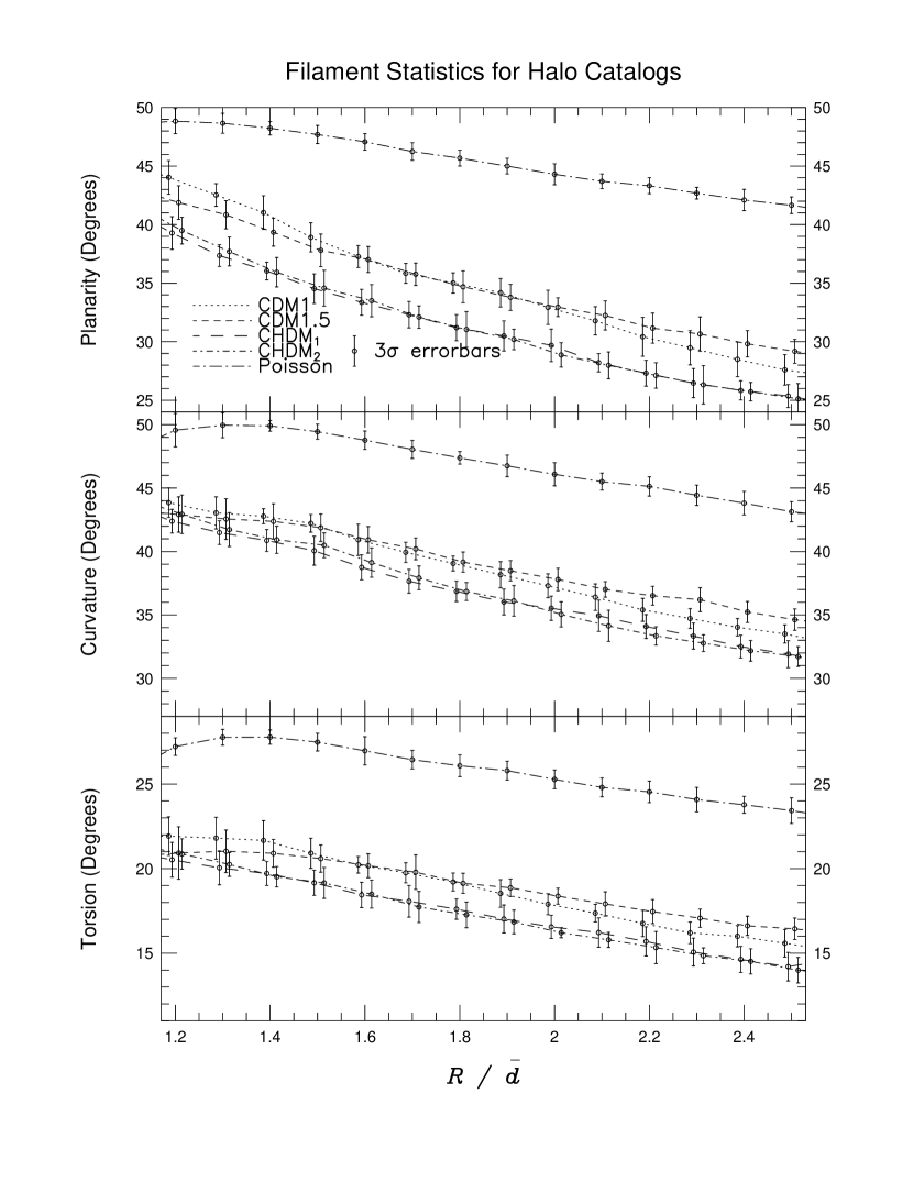
Figure 2: Halo Catalogs Filament Stats

Figure 2 shows the results for filament statistics planarity $\bar{\theta}_{P}$, curvature $\bar{\theta}_{C}$, and torsion $\bar{\theta}_{T}$ vs. $R/\bar{d}$ applied to the halo catalogs catalogs after breakup. The statistics were computed for each $R/\bar{d}$ from 1.2 to 2.5 in increments of 0.1. To estimate errors in the halo catalogs, each statistic was computed over a random subset of the catalog. The subset was taken to be as many halos as necessary to generate 500 link sequences. Even for $R/\bar{d}=1.2$, this never required more than 650 halos; at high $R$, hardly a few percent of the halos generated sequences which did not meet the $N_{L,min}=4$ criterion. The error bars shown in Figure 2 are $3\sigma$ resampling errors. The catalog was then resampled 10 times to obtain an error estimate. Since there are more than 34,000 halos in each catalog, the data is not oversampled. At $R/\bar{d}=1.2$, there were on average 5.6 links per sequence; this number rose steadily until $R/\bar{d}\geq 1.6$, where sequences were was almost always terminated due to the $N_{L,max}={100\;{\rm Mpc}/\bar{d}}\approx 34$ criterion. The average number of halos within a sphere of radius $R$ around a given sequence point rose from $\sim$10 at $R/\bar{d}=1.2$ roughly linearly to $\sim$50 at $R/\bar{d}=2.5$.

Figure 2 shows that all three statistics are generally higher for the CDM simulations as compared with the CHDM simulations, indicating that CDM is less filamentary, has fewer sheet-like structures, and has greater clumpiness than the CHDM simulations. These results are consistent with the notion that CDM possesses more evolved structures with clumpier mass distributions, while the presence of neutrinos in CHDM models results in more extended and less evolved structures This notion is confirmed by the visualizations of BHNPK. Thus filament statistics provide quantitative differentiation between large-scale structure seen in the halo catalogs.

Note that all the statistics tend to fall with increasing $R$. This reflects the fact that as the ratio of ${R/L}$ increases, the greater overlap between adjacent spherical windows generates stronger correlations between adjacent inertia tensors, thereby reducing the angle deviations between neighboring inertia ellipsoid axes. There is an additional effect that is peculiar to catalogs possessing inherent filamentary structure: Consider a link sequence tracing a path defined by points contained in a “filamentary structure” of radius $R_{cyl}$. As we increase ${R/L}$ we see an increasingly more linear distribution of points in the window, thus lowering the value of ${\bar{\theta}_{C}}\sim\frac{1}{2}\arcsin(R_{cyl}/{R})$. A similar argument holds for planarity and torsion. In reality the galaxy distribution is more complex, but the basic result is that sampling large-scale structure gives ${\bar{\theta}_{C}}(R)$, ${\bar{\theta}_{P}(R)}$, and ${\bar{\theta}_{T}(R)}$ falling at rates greater than in the Poisson case.

The large difference between simulations and the Poisson catalogs provides a good indicator of how effectively structure is identified by filament statistics. Link sequences identify and follow structure in a Poisson catalog by detecting chance alignments of halos which masquerade as contiguous structure due to finite numbers of halos in a given window. As mentioned before, this structure aliasing is primarily a low-galaxy-density phenomenon, and hence is most significant at low $R$, where all sequences barely exceed $N_{L,min}$, and each window barely has $N_{P,min}$ halos. In this situation the majority of sequences which qualify will be those lying along such rare chance alignment of halos. Increasing $N_{P,min}$ and $N_{L,min}$ reduces structure aliasing, but the corresponding reduction in qualifying sequences increases shot noise significantly. Instead, we simply choose to be careful about our interpretations at low $R$. For instance, for $R/\bar{d}\leq 1.3$ the Poisson catalog statistics rise with $R$, indicating that aliased structure is significant here. Structure aliasing occurs in the models as well, but is less apparent because halos are correlated, yielding more halos surrounding a given point than in the Poisson case. Nevertheless the reduced discrimination for $R/\bar{d}\leq 1.3$ is an indication that aliased structure is of comparable strength to real structure at these scales.

At low and high $R$ values, filament statistics discriminate between the CDM models with different biases, as shown in Figure 2. At $R/\bar{d}\leq 1.3$ CDM1.5 aliases structure more effectively than CDM1 since it is more diffuse (more Poisson-like), while at larger scales ($\ga 7$ Mpc) the enhanced clustering of CDM1.5 (see BHNPK) tends to trap sequences in spherical clumps more effectively than CDM1, giving higher values. Identification of these effects over a $R$ of 1.0–2.5 (roughly 3.0–7.5 Mpc) indicates the high sensitivity of these statistics to the presence of structure.

The two CHDM simulation results are within $\sim 1\sigma$ of each other on scales investigated. Hence for these statistics, cosmic variance between CHDM₁ and CHDM₂ should be comparable to resampling errors in the halo catalogs.

5.2 Shape Statistics Applied to Halo Catalogs

We applied the BS, LV, and RA statistics to the halo catalogs after breakup. To compare with filament statistics, we took ten sets of 1000 eligible halos each to compute resampling errors, varying the window radius $R$ from $1.2\bar{d}$ to $2.5\bar{d}$. Eligible halos were those which had five or more other halos within the selected radius $R$, analogous to the filament statistics computation. BS points out that at least 12 halos are required within a window radius to avoid structure aliasing and reliably identify a planar structure; however, for such a high value, few halos are eligible and hence shot noise reduces the discriminatory power significantly. Lowering this number to three increases the discriminatory power slightly, but structure aliasing becomes more significant at small scales. The results for $LV_{\sl quad}$ and $LV_{\sl plane}$ along with the $RA$ statistic applied to the halo catalogs after breakup are shown in Figure 3, while the results for the $BS$ statistics are shown in Figure 4. We omit $LV_{\sl line}$ for redundancy; it gives lower discrimination than $LV_{\sl plane}$ but otherwise has very similar behavior. The error bars shown are 3$\sigma$ resampling errors.

For $R/\bar{d}\leq 1.5$, the Poisson model is poorly discriminated from the cosmological models for all statistics. This is due to strong structure aliasing in these small windows ($R\la 5$ Mpc), making the statistics clearly untrustworthy at these scales. To avoid these spurious detections of structure we focus on the regime $R/\bar{d}\geq 1.6$. Recall that for filament statistics, structure aliasing was problematic only for $R/\bar{d}\la 1.3$, so filament statistics are able to discriminate true structure from aliased structure at smaller scales.

For $R/\bar{d}\geq 1.6$, the results of the shape statistics are consistent with BHNPK visualizations. CHDM models show higher filamentarity ($BS_{\sl prol}$ and $LV_{\sl quad}$) and planarity ($BS_{\sl obl}$, $LV_{\sl plane}$, and $RA$) than CDM models, while the sphericity measure $BS_{\sl sph}$ is higher for the CDM models. However, CDM1.5 is generally closer to the CHDM models until $R/\bar{d}\ga 2.0$. Comparing the values for $BS_{\sl prol}$ and $BS_{\sl obl}$ show that the halo distribution is more oblate than prolate, i.e. that large-scale structure in these models is dominated by sheets rather than filaments. A comparison of $LV_{\sl plane}$ and $LV_{\sl line}$ (not shown) yields the same conclusion. Thus these shape statistics, like filament statistics, confirm and quantify the visually apparent differences between these models.

As $R/\bar{d}$ increases, the errors become smaller primarily due to more halos being included within each window. The statistical values also decrease partly due to a reduction in structure aliasing, and partly because larger windows tend to sample more spherical mass distributions.

All statistics appear to be fairly sensitive to the chosen bias as well as the chosen set of initial conditions. CDM1 is well discriminated from CDM1.5 except in the region around $R/\bar{d}\sim 2.5$ where their curves intersect; CDM1, being the more evolved model, contains less filamentary and planar structure at small scales. For the LV statistics and $BS_{\sl sph}$, the cosmic variance estimated from the difference between CHDM₁ and CHDM₂ begins to dominate over resampling errors for $R/\bar{d}\ga 2.0$, while the $RA$ and $BS_{\sl obl}$ shows $\ga 2\sigma$ cosmic variance at all scales. Only for $BS_{\sl prol}$ is the cosmic variance always comparable to the resampling error for $R/\bar{d}\geq 1.6$.

In comparison with filament statistics, the shape statistics give the same conclusion regarding structure formation in the various models, but appear to have more sensitivity to cosmic variance (with the exception of $BS_{\sl prol}$), and are more susceptible to structure aliasing at small scales. The large difference between CDM1 and CDM1.5 indicates shape statistics are more sensitive to the normalization of the cosmological model than filament statistics; to some degree, this makes shape statistics a complementary diagnostic.

5.3 Measuring the Discriminatory Power

We now introduce a set of metastatistics to compare statistics and assess the effectiveness of our analysis. These metastatistics will allow a direct comparison of the discriminatory power and robustness of filament statistics versus shape statistics. Discrimination between models for a given statistic $\theta$ can be measured by the signal strength $S^{\theta}_{\rm res}$ between catalogs:

$$S^{\theta}_{\rm res}(1,2)={{|\theta_{1}-\theta_{2}|}\over{\sqrt{\sigma_{\theta_{1}}^{2}+\sigma_{\theta_{2}}^{2}}}}$$ (12)

where $\theta_{1}$ and $\theta_{2}$ are values of statistic $\theta$ for catalogs 1 and 2, respectively, and $\sigma_{\theta}$ is the resampling error for that statistic and catalog. The subscript “res” denotes that the units of $S^{\theta}_{\rm res}$ are $1\sigma$ resampling errors. To compare CHDM to CDM at (roughly) COBE normalization while excluding cosmic variance, we compare CHDM₁ to CDM1. Figure 5(a) shows $S^{\theta}_{\rm res}$(CDM1,CHDM₁) for the halo catalogs for $\theta=\{\bar{\theta}_{P},\bar{\theta}_{C},\bar{\theta}_{T}\}$. computation) For $R\geq 1.4$, where structure aliasing is unimportant, planarity shows the highest signal, then curvature then torsion, with all statistics showing $S^{\theta}_{\rm res}$(CDM1,CHDM₁)$\ga 4\sigma$. Thus filament statistics are fairly discriminatory for the halo catalogs; their robustness against halo breakup will be formally investigated in §5.4. Cosmic variance is not expected to dramatically degrade the discrimination as the differences between CHDM₁ and CHDM₂ are comparable to the resampling errors.

The signal strengths for the LV, BS, and RA statistics applied to the halo catalogs after breakup are shown in Figure 5b (bottom panel). For most statistics, discrimination is better than $5\sigma$ for $R/\bar{d}\geq 1.6$. The significant exception is $BS_{\sl prol}$, with barely $\sim 2-3\sigma$ discrimination for $R/\bar{d}\geq 1.8$. However, recall that $BS_{\sl prol}$ was also the only statistic whose cosmic variance was small compared with resampling errors. With cosmic variance taken into account, $BS_{\sl prol}$ appears to be quite comparable in discriminatory power to the other statistics. In general, both filament and shape statistics appear to be easily discriminate structure formation in CDM models versus CHDM models. Cosmic variance, though, appears to be more of a concern for the shape statistics, with the exception of $BS_{\sl prol}$.

5.4 Robustness Against Halo Breakup

The identification of galaxies in simulations represents a major uncertainty in this type of analysis. Given that the simulations are dissipationless, it is not possible to directly identify clumps of baryons which would be expected to form galaxies. Instead, assumptions must be made regarding how the baryonic matter traces the dark matter. In addition, because of the limited resolution of the simulations, a single clump of dark matter may contain several galaxies (often referred to as the “overmerging problem”), and must be broken up to obtain a true sample of galaxies. The detailed assumptions made in this procedure (described in NKP96) are somewhat ad hoc, so it is important to somehow quantify the uncertainty introduced by our lack of knowledge.

To do this we compare the statistical values for the catalogs before breakup and after breakup. The effects of breakup on these statistics are expected to be as follows: Because single halos are broken into several spherically-distributed halos, the tendency will be to decrease the detection of planar and filamentary structure, and increase the detection of spherical structure. This is in fact what is seen. Since it is clear some sort of halo breakup must be done, and that halo breakup has a monotonic effect on the statistics, a comparison of catalogs before and after breakup should yield a somewhat conservative estimate of the uncertainty introduced by this procedure, unless the breakup scheme used here produces far too few fragments.

We first measure the halo identification uncertainty factor, given by

$$F_{\rm id}(\theta)=\left\langle{{|\theta{\rm bu}-\theta{\rm nobu}|}\over{\sqrt{(}{\sigma_{\theta{\rm bu}}}^{2}+{\sigma_{\theta{\rm nobu}}}^{2})}}\right\rangle_{{\rm cats}}$$ (13)

where $\theta$ represents the value of the statistic in question, $bu$ and $nobu$ refer to breakup and no-breakup catalogs, and $\sigma_{\theta}$ represents the resampling error for statistic $\theta$. We then combine this error with resampling errors to obtain the combined signal strength metastatistic, presented as a function of radius $R$:

$$S^{\theta}{\rm res+id}(1,2)={{S^{\theta}{\rm res}(1,2)}\over{MAX[1.0,F_{\rm id}(\theta)]}}$$ (14)

For the filament statistics applied to the halo catalogs, we compute $S^{\theta}_{\rm res+id}({\rm CHDM}_{1},{\rm CDM}_{1})$ for each statistic for $R=1.2-2.5$. The results are plotted in Figure 6(a) (top panel). Torsion show no degradation of signal, as $F_{\rm id}(\theta_{T})<0.4$ for all values of $R$; this statistic is highly robust against halo identification uncertainty. Curvature, conversely, shows some degradation, as it typically has $F_{\rm id}(\theta_{C})\sim 1.7$. Planarity, which showed the highest signal strength, is by far the least robust, with $F_{\rm id}(\theta_{C})\sim 2$ and as high as 2.5 at some values of $R$. Comparing with Figure 5(a), torsion now appears marginally to be the best filament statistic, showing typically $4\sigma$ robust discrimination between models, while curvature and planarity have $S^{\theta}_{\rm res+id}({\rm CHDM}_{1},{\rm CDM}_{1})\sim 3$. Recall from Figure 2 that all statistics show CHDM₁ and CHDM₂ being $\la 1\sigma$ apart, so these conclusions should not be dramatically affected by cosmic variance.

Figure 6b (bottom panel) shows the combined signal strengths computed shape statistics applied to the halo catalogs. For all the statistics except $RA$, the results are generally insensitive to breakup. For $RA$, $F_{\rm id}\sim 1.5$ typically, but it still leaves $RA$ with comparable discriminatory power as other shape statistics. While no shape statistic is clearly optimal by this measure, $BS_{\sl obl}$, $BS_{\sl sph}$, and $LV_{\sl plane}$ appear to show the strongest discrimination; however cosmic variance is a concern for those statistics. $BS_{\sl prol}$, which had low cosmic variance, is not very discriminatory. Overall, there are statistics from each category showing over $4\sigma$ discrimination which is robust against variations in the galaxy identification scheme.

6 Results For Sky Catalogs

6.1 The Effect of Redshift Distortion

Distortion of structure due to peculiar motions of individual galaxies (e.g. fingers of God) could in principle significantly degrade the ability of all of these statistics to quantify true structure. In our case, since CDM contains higher peculiar velocities, one might expect stronger fingers of God which could mimic the true filamentarity contained in CHDM and thereby work against the discriminatory power of these statistics. This does not turn out to be the case, however, because fingers of God are elongated only in the line-of-sight direction r̂ in redshift space, whereas in general a structure in real space will not be aligned with r̂. Thus redshift distortion tends to smear out and hence decrease the amount of structure detected in these simulations, slightly more so in models with more redshift distortion. For filament statistics, a further effect of redshift space distortion is to misguide sequences and increase the angle deviation of a sequence passing through a cluster. The net result is that redshift distortion does not significantly undermine the ability of any of these statistics to distinguish between cosmological models, and in some cases slightly enhances the discrimination.

To test the effect of redshift distortion we adopt the strategy of applying the statistics to mock redshift catalogs constructed to exaggerate the distortion due to peculiar velocities. We first cut the halo catalogs at a high density threshold, roughly mimicking CfA1 sparseness. Then for each halo we compute the line-of-sight velocity ${\rm v}_{\rm los}$ with respect to an observer at one corner of the simulation volume. We then multiply this velocity by $F_{V}$, the velocity scaling factor, and shift the halo position along the line of sight by

$$\Delta{\bf x}=F_{V}{\rm v}_{\rm los}\Delta\hat{\bf r}/H_{0}$$ (15)

where $\Delta\hat{\bf r}$ is the direction from the box center to the given halo. Thus $F_{V}=0$ corresponds to real space, $F_{V}=1$ corresponds to redshift space, while higher $F_{V}$ yields an exaggerated shift from which we can gauge the sensitivity of the statistics to redshift distortion. We choose $R/\bar{d}=1.5$ when applying the test to filament statistics, and $R/\bar{d}=1.8$ when testing the other shape statistics.

Figure 7(a) (left side) shows the effect of the transformation from real to redshift space upon filament statistics for halo catalogs with a density threshold of ${\delta\rho}/{\rho}>80$, while Figure 7(b) (right side) shows the equivalent results for ${\delta\rho}/{\rho}>120$ catalogs. At $F_{V}=1$, we see a definite increase in the discrimination between the models as compared to $F_{V}=0$, most notably for the curvature and torsion statistics. This effect is more pronounced in the sparser catalogs. The statistical values increase, indicating structure is being smeared out by redshift distortion. The trend continues to higher $F_{V}$, with no dramatic dropoff in the discriminatory power of filament statistics. This test was also run on the pre-breakup versions of the same catalogs, and it was found that the interpretations are virtually independent of breakup in both real and redshift space.

Figure 8 shows the results of the redshift distortion test for three selected shape statistics (the others show similar behavior). As with filament statistics, less structure is detected when redshift distortion is included. Unlike filament statistics, however, there is no apparent increase in the disriminatory power of these statistics at $F_{V}=1$. Also, exaggerated redshift distortion ($F_{V}\geq 2$) has little further effect on the statistics. Again, these results are fairly insensitive to breakup and catalog density.

In summary, the primary effect of redshift distortion is to decrease strength of structure, which if anything will work to amplify the discrimination between the models considered. Filament statistics, which emphasize regions of higher density, are more affected by redshift distortion than the randomly-sampled shape statistics, and we see greater amplification of discrimination between models.

6.2 Filament Statistics Applied to Sky Catalogs

Figure 9 shows the results of filament statistics applied to the sky catalogs after halo breakup. Every galaxy in each sky catalog was tried as a possible sequence starting point. For each catalog, at $R=1.2$, around 800 of the $\approx$2360 galaxies typically generated sequences with number of links exceeding $N_{L,min}=4$. This number rose roughly linearly until $R=2.5$, where $\sim$2200 galaxies qualified, on average, in each catalog. There were systematic differences between the catalogs as well, with CHDM₂ showing the largest number of accepted sequences, about $5-10\%$ more than the CDM models. CHDM₁ showed the lowest number, consistently slightly below the CDM models. At $R=1.2$, there were on average about 6 links per sequence; this number rose fairly linearly with $R$, such that at $R=2.5$, there were around 20 links per sequence. The average number of galaxies within a sphere of radius $R$ around a given sequence point rose from 8–10 at $R=1.2$ roughly linearly to 25–30 at $R=2.5$.

The error estimate for each statistic in sky catalogs was determined from sky variance, by computing the statistic at each of six vantage points, and getting an average value and standard deviation for that statistic. The error bars shown in Figure 9 are $1\sigma$ sky variance errors. Since our box is relatively small, different viewpoints are still seeing many of the same structures, although with differing depth. Sky variance is therefore expected to underestimate true cosmic variance, perhaps significantly.

Figure 9 shows that both CHDM models still show more structure than either CDM model, consistent with our intuitive picture of structure formation in these models, and all models are fairly well discriminated from the Poisson catalog. However, CHDM₁ shows significantly more structure than CHDM₂, by up to $\sim 2\sigma$ for the torsion and curvature statistics, indicating that that sky variance is an inadequate estimate of cosmic variance. The extra large scale power in CHDM₁, accentuated by the artificial replication of structure in the construction of the sky catalogs at 100 to $100\sqrt{3}$ Mpc intervals, produces more large-scale structure in CHDM₁ than in CHDM₂. This is more apparent in sky catalogs than in the halo catalogs since the scales investigated are much larger, with $\bar{d}\sim 10$ Mpc even in the region where the sky catalogs are complete.

To test sensitivity to shot noise and catalog boundary effects, filament statistics were applied to (nearly) full-sky versions of the CfA1-like sky catalogs with a zone of avoidance $|b|\leq 10^{\circ}$ about each viewpoint, covering 10.384 sr instead of 2.66 sr and containing about four times as many galaxies ($\approx 9200$). Since the 2.66 sr catalogs and the 10.384 sr catalogs are derived from the same simulation data set, we are still sampling from the same distribution of cluster sizes and shapes. The resulting signal strength increased by a factor of $\sim 2$ (for $R/\bar{d}\geq 1.3$) as expected if the errors are dominated by shot noise. The degradation of the signal from the halo catalogs to the sky catalogs is thus primarily due to sparseness. For a survey such as the Optical Redshift Survey (Santiago et al. 1995,1996) which covers 8.09 sr at CfA1 depth, we expect to see well over $3\sigma$ discrimination between models, excluding cosmic variance.

We quantify boundary effects by comparing statistical values for the 2.66 sr catalogs vs. the 10.384, and find that for $R/\bar{d}\ga 2.0$, the CfA1-like catalogs show significantly higher values (comparable to sky variance) than the 10.384 sr catalogs, indicating that the entire catalog volume was contributing as a single radial filamentary structure. This was also evident from visualizations of the link sequences, as at large $R$ the sequences were preferentially radially directed. Visualization also showed that link sequences were distributed throughout the sky catalog volume, with very few lying in the foreground, $r\la 20$ Mpc. Recall that $\bar{d}(r)$ is small at low $r$, and the Virgo Cluster, being nearby, contributes hardly any sequences even though it gives a large finger of God. At small $R$, sequences tended to be shorter and terminate within the catalog volume, while at large $R$ they tended to terminate once they exceed the catalog boundary and find no nearby galaxies.

The statistics were also applied to 80 Mpc volume-limited versions of the sky catalogs, with typically 400-500 galaxies in each. The statistics showed very large shot-noise scatter, and gave no significant discrimination between models. Volume limiting certainly yields more interpretable statistics, but for CfA1 and our similar-size simulation sky catalogs, there are simply too few galaxies.

6.3 Shape Statistics Applied to Sky Catalogs

In Figure 10 we present the (selected) $LV$ and $RA$ statistics and in Figure 11 the $BS$ statistics, applied to the sky catalogs after halo breakup. Also plotted as solid lines are the results for the CfA1 catalog. Each statistic was computed around every galaxy in the sample. The errors are increased greatly over the halo catalog case because of the sparseness of these CfA1-like catalogs; the error bars shown are $1\sigma$ sky variance errors.

The interpretation of statistical values again confirms the intuitive picture of structure formation in these models. CHDM models show greater filamentarity and planarity and less sphericity than CDM models for $R/\bar{d}\ga 1.5$. As with the halo catalogs, the galaxy distribution shows stronger planarity than filamentarity, with $BS_{\sl obl}$ typically twice $BS_{\sl prol}$ at any given $R$. Also, the CDM models show different trends versus $R$ analogously to the halo catalogs, with CDM1.5 dropping faster versus $R/\bar{d}$ than CDM1.

For the LV and RA statistics applied to the sky catalogs (Figure 10), structure aliasing is a significant concern. The Poisson catalog is not discriminated from the models until the scales are quite large, $R/\bar{d}\sim 1.8$ for $LV_{\sl quad}$ and $RA$. The higher order LV statistics (represented in Figure 10 by $LV_{\sl plane}$; $LV_{\sl line}$ and $LV_{\sl flat}$ show similar behavior) are never well discriminated from the Poisson catalog. As with the halo catalogs, filament statistics do a better job avoiding aliased structure at small scales. The CHDM models are well separated, indicating that cosmic variance dominates over sky variance for these statistics. In all, the LV and RA statistics appear less able to reliably quantify structure than filament statistics in a catalog as sparse as CfA1.

The BS statistics (Figure 11) do not have quite as much difficulty distinguishing a Poisson catalog from the cosmological models as the LV and RA statistics, although they still cannot discriminate for $R/\bar{d}\leq 1.5$. $BS_{\sl prol}$, just as in the halo catalog case, shows remarkable little cosmic variance for $R/\bar{d}\ga 1.8$, although with only two realizations of CHDM the possibility that this is merely a fortuitous coincidence cannot be ruled out. For $BS_{\sl obl}$ and $BS_{\sl sph}$, cosmic variance is again a significant source of uncertainty, with CHDM₁ generally closer to the CDM models than CHDM₂.

We also applied these statistics to the full-sky versions (10.384 sr) of the sky catalogs. The discriminatory power of the best statistics increased only to $\sim 3\sigma$, showing that these statistics are not completely dominated by Poisson noise, and are more affected by halo identification uncertainty than filament statistics. As with filament statistics, boundary effects become significant for $R/\bar{d}\ga 2.0$.

6.4 Robustness and Discrimination Between Models

In Figure 12 we present the combined signal strength $S^{\theta}_{\rm sv+id}$(CDM1,CHDM₁) for all the statistics applied to the sky catalogs. The subscript “sv” signifies that we are including sky variance errors. The results before breakup are not shown, but for most statistics, the sparseness of the CfA1 catalog generates sky variance errors which dominate over halo identification uncertainty, so $F_{\rm id}<1$ at nearly all $R$. The exception is the $RA$ statistic, which had $F_{\rm id}\sim 1.5$ typically. As described in section 4.3 the catalogs before breakup show slightly more structure than after breakup. It turns out that for filament statistics, this represents a $\la 1^{\circ}$ increase in each statistic for the sky catalogs, which is generally less than sky variance errors. There is little qualitative difference in $S^{\theta}_{\rm sv+id}$(CDM1,CHDM₁) for no-breakup sky catalogs.

Figure 12(a) shows that for filament statistics, discrimination between CHDM₁ and CDM1 is strongest in torsion ($\sim 2.5\sigma$) and curvature ($\sim 1.5-2\sigma$), while planarity shows no significant discrimination between CHDM and CDM. Planarity is weaker because it is not as significantly amplified by redshift distortion as curvature and torsion, as was described in §6.1 (see Figure 7(b)). While promising, these levels of discrimination are comparable to our crudely estimated cosmic variance.

The signal strengths $S_{\rm sv+id}$(CHDM₁,CDM1) for the shape statistics applied to the sky catalogs after breakup are shown in Figure 12b (bottom panel). Greatest discrimination is seen for $BS_{\sl prol}$, at a modest $\sim 1.5-2\sigma$ level for $1.7\la R/\bar{d}\la 2.2$. The $LV_{\sl line}$ statistic shows some apparent discrimination at $R/\bar{d}\sim 1.5$, but recall for this $R$ this statistic does not discriminate a Poisson catalog from the cosmological models. None of the other statistics show significant discrimination between these models.

Overall, we conclude that for the CfA1-like sky catalogs, the best filament statistic is torsion, which clearly has the greatest discriminatory power of any statistic with the caveat that it may be significantly degraded by cosmic variance. Of the shape statistics, the Babul & Starkman prolateness measure $BS_{\sl prol}$ gives the most discrimination between models when applied to a CfA1-like data set, showing some discriminatory power (up to $2\sigma$) and good robustness against both halo identification uncertainty and cosmic variance. The LV and RA shape statistics show little discriminatory power between models or even from a Poisson catalog in such a sparse survey. Testing on 10.384 sr versions of the sky catalogs shows that all these statistics are hampered mostly by shot noise, thus a larger data set is required to properly discriminate between these models. The Optical Redshift Survey (Santiago et al. 1995, 1996) which has CfA1 depth but 8.09 sr sky coverage, will be very useful for this purpose.

6.5 Comparing Models vs. CfA1 Data

Using these statistics we can compare the sky catalog results directly to CfA1 data. For filament statistics shown in Figure 9, the CfA1 catalog follows the CDM models more closely than the CHDM models. However, given the uncertainty in halo identification ($\sim 1^{\circ}$) and cosmic variance, it is difficult to conclusively state which model agrees best with filament statistics based on the CfA1 data set.

The various shape statistics presented in Figures 10 and 11 likewise show that no single model of those considered here is completely consistent with CfA1 data. The LV and RA statistics show best agreement with CHDM₁, but these statistics have large cosmic variance. $BS_{\sl obl}$ and $BS_{\sl sph}$ show best agreement with the CHDM models, while $BS_{\sl prol}$ shows best agreement with the CDM models. With at best $2\sigma$ discrimination combined with the uncertainties in our estimates of cosmic variance and halo identification robustness, we again cannot favor or rule out any models based on these shape statistics applied to the CfA1 redshift survey.

7 Conclusions

In this paper we present filament statistics, a new set of statistics for quantifying filamentarity and planarity in large-scale structure. We compare these statistics to the shape statistics of Babul & Starkman (1992), Luo & Vishniac (1995), and Robinson & Albrecht (1996) by introducing metastatistics which quantify the discriminatory power and robustness of each statistic. We find that when applied to the halo catalogs, most of the statistics considered are sensitive and robust diagnostics of large scale structure that effectively discriminate simulations of CDM models from simulations of CHDM models, with robust discrimination of $\ga 4\sigma$ between CDM and CHDM models. Cosmic variance is low for the filament statistics, but more of a concern for all the shape statistics except perhaps $BS_{\sl prol}$. The signal-to-noise ratio between any model and the Poisson catalog is very large for all $R\geq 1.5\bar{d}$, where $R$ is the window radius and $\bar{d}$ is the mean intergalaxy spacing. Finally, all statistics show that CHDM contains more sheet-like and filamentary structures than CDM, consistent with intuitive expectations as well as visualizations done by BHNPK.

Comparison with redshift survey data must be done in redshift space with the appropriate survey geometry. We compare CDM and CHDM models to CfA1 data by utilizing a sample of CfA1-like redshift catalogs constructed from each of the simulations, and comparing these “sky catalogs” directly to the CfA1 survey. When one views the statistics’ results for sky catalogs, it is unclear which statistic provides the most discrimination between models. Filament statistics tend to show better robust discrimination than the shape statistics, but cosmic variance is a concern. Comparing models to CfA1, we find the filament statistics show, at face value, that the CDM simulations provide the best fit to CfA1 data. On the other hand, for most shape statistics the CHDM models appear to be a better fit. In all cases the discrimination is poor, and significantly weakened by uncertainties in halo identification as well as cosmic variance. A proper comparison of statistics and of models versus redshift survey data must await larger data sets.

In a broad context, we view filament statistics as illustrative of a new methodology for constructing statistics to analyze spatial data. We utilize inertia tensors to characterize the local mass distribution, similarly to the LV, BS, and RA statistics. But rather than deriving combinations of tensor moments to quantify structure, filament statistics use link sequences to generate new data samples which amplify properties of interest in the underlying data set. The link sequence approach was conceived of as an intuitive means of simplifying the complex topology of the galaxy point set while enhancing the sense of approximate connectivity of its large-scale isodensity surfaces (which the eye might recognize as “filamentarity”). Since the link sequences are guided by the distribution of galaxies, not bound by it (as in Delaunay or Voronoi tessellations, see e.g. van de Weygaert 1991, or minimal spanning trees, see e.g. Pearson & Coles 1995), they are more likely to be robust against variations in the galaxy locations and halo breakup, although as we have seen, robustness against galaxy identification in magnitude-limited mock redshift catalogs is a trickier issue. Another approach for using link sequences is to apply shape statistics like those of LV, BS, and RA to the newly created data sample, producing statistics which may be more discriminatory than any presented here. We plan to investigate this possibility in the future.

The success of these statistics for the halo catalogs indicates that larger, denser redshift surveys coupled with larger simulations will provide a significant increase in the robustness and discriminatory power of these statistics versus real survey data. A proliferation of such large redshift surveys is already underway. On the simulations front, good progress is being made in scaling up the size and resolution of cosmological simulations, as well as in constructing constrained realizations of the local universe (Primack 1995) by which one may avoid uncertainties of cosmic variance. Thus we soon hope to have a suite of significantly larger simulations of currently favored models which we can compare to these large redshift surveys. Finally, there is interesting work being done in more realistically handling the overmerging problem by combining approximations to hydrodynamics with Press-Schecter type formalisms to accurately model the numbers of galaxies near the resolution limit of the simulations (Kauffman, Nusser & Steinmetz 1995; Somerville et al. 1996, in preparation). In the coming years we hope to establish these statistics which quantify the shapes of large-scale structure as significant constraints on cosmological models of structure formation.

Table 1: Halo catalogs (KNP96,NKP96)

Model	$\Omega_{c}/\Omega_{\nu}/\Omega_{b}$	Bias	Qrms($\mu$K)	Init.Cond.	No. of Gals.	$\bar{d}$ (Mpc)
CDM1	$1.0/0/0$	$b=1.0$	12.8	Set 1	58,121(37,164)	2.58(3.00)
CDM1.5	$1.0/0/0$	$b=1.5$	8.5	Set 1	61,690(45,592)	2.53(2.80)
CHDM1	$0.6/0.3/0.1$	$b=1.5$	17.0	Set 1	34,000(29,151)	3.09(3.25)
CHDM2	$0.6/0.3/0.1$	$b=1.5$	17.0	Set 2	34,554(29,765)	3.07(3.23)

The number of galaxies and mean interparticle spacing $\bar{d}$ computed before halo breakup are indicated in parentheses.

Table 2: Shape statistics test cases: Line, Plane, and Sphere

Stat	Line	Plane	Sphere
$LV_{\sl quad}$	0.976/0.989 (1)	0.269/0.254 (0.25)	0.012/0.006 (0)
$LV_{\sl line}$	0.953/0.978 (1)	0.035/0.008 (0)	0.004/0.002 (0)
$LV_{\sl plane}$	0.000/0.000 (0)	0.906/0.978 (1)	0.029/0.014 (0)
$LV_{\sl flat}$	0.953/0.978 (1)	0.959/0.989 (1)	0.033/0.015 (0)
$BS_{\sl prol}$	1.000/1.000 (1)	0.016/0.002 (0)	0.004/0.002 (0)
$BS_{\sl obl}$	0.000/0.000 (0)	0.959/0.991 (1)	0.012/0.001 (0)
$BS_{\sl sph}$	0.000/0.000 (0)	0.000/0.000 (0)	0.909/0.977 (1)
$RA$	0.000/0.000 (0)	0.659/0.743 (1)	0.168/0.063 (0)

Values of individual statistics for three test case random distributions. The first value is for $R=5$ Mpc, the second is for $R=10$ Mpc, and the value in paranthesis is the analytical value for that distribution.

Captions

Figure 1. Link sequence generation computational flowchart. $R$ is taken in units of the mean intergalactic spacing $\bar{d}$. For galaxies in redshift space, $\bar{d}$ is a function of the Hubble distance $r=v/H_{0}$, where $v$ is the radial velocity of the galaxy. From the initial galaxy, sequences are propagated in both (opposing) directions along the major axis until termination; if the combined number of links is 4 or more, the entire (combined) sequence “qualifies” for computation; else it is discarded.

Figure 2. Filament statistics (planarity $\bar{\theta}_{P}$, curvature $\bar{\theta}_{C}$, and torsion $\bar{\theta}_{T}$) for the halo catalogs versus $R/\bar{d}$, with $L=\bar{d}$. Error bars shown are $3\sigma$ resampling errors. The statistics show the CHDM models having more structure than the CDM models, by well over $4\sigma$ at most $R$. Cosmic variance estimated by the difference between CHDM₁ and CHDM₂ is generally comparable to resampling error. The Poisson catalog is well discriminated from any model for $R/\bar{d}\geq 1.3$. Note: Values for different models are slightly offset in $R$ to improve visibility.

Figure 3: Results for selected Luo & Vishniac (1995) statistics and the Robinson & Albrecht (1996) statistic applied to the halo catalogs after halo breakup. Error bars shown are $3\sigma$ resampling errors. The cosmological models are well discriminated from the Poisson model for $R/\bar{d}\geq 1.6$. The statistics are sensitive to the cosmological model as well as to the normalization (i.e. the bias factor), with CDM1 and CDM1.5 showing markedly different trends with $R$. Cosmic variance seems to be significant for all these statistics, indicating that resampling errors may not be an appropriate measure of total variance.

Figure 4: Results from the Babul & Starkman (1995) statistics applied to the halo catalogs after halo breakup. Error bars shown are $3\sigma$ resampling errors. These statistics generally show a very similar behavior versus each other and versus the Poisson catalog as the $LV$ statistics. The exception is $BS_{\sl prol}$, which shows very little cosmic variance for $R/\bar{d}\geq 1.8$.

Figure 5. (a) Signal strengths $S^{\theta}_{\rm res}$(CHDM₁,CDM1), as defined in equation 12, for $\bar{\theta}_{P}$, $\bar{\theta}_{C}$, and $\bar{\theta}_{T}$ applied to the halo catalogs. All statistics discriminate fairly well, with planarity showing the most discrimination. (b) Signal strengths $S^{\theta}_{\rm res}$(CHDM₁,CDM1) for the shape statistics applied to the halo catalogs. All statistics show good discriminatory power, with the best ones exceeding $\sim 8\sigma$.

Figure 6. Combined signal strengths $S^{\theta}_{\rm res}$(CHDM₁,CDM1) as defined in equation 14; compare to Figure 5 to see effect of breakup. (a) $S^{\theta}_{\rm res+ID}$(CHDM₁,CDM1) for the filament statistics applied to the halo catalogs. Comparison with Figure 5(a) shows that breakup causes the most degradation for planarity, some for curvature, and none for torsion. (b) $S^{\theta}_{\rm res+ID}$(CHDM₁,CDM1) for the shape statistics applied to the sky catalogs. All statistics are quite robust with respect to halo identification uncertainty, with the exception of $RA$.

Figure 7. Filament statistics $\bar{\theta}_{P},\bar{\theta}_{C},\bar{\theta}_{T}$ applied to mock-observed (a) ${\delta\rho/\rho}>80$ and (b) $\delta\rho/\rho>120$ halo catalogs with velocities scaled from velocity factor $F_{V}=0$ (real space) to $F_{V}=5$ times their actual value, with $R/\bar{d}=1.5$. Error bars shown are $1\sigma$ resampling errors. Going from real space ($F_{V}=0$) to ordinary redshift space ($F_{V}=1$) decreases the amount of structure detected, but actually increases discrimination between models. Note: Values for different models are slightly offset in $F_{V}$ to improve visibility.

Figure 8: Redshift distortion test applied to catalogs cut at ${\delta\rho\over\rho}\geq 80$ and ${\delta\rho\over\rho}\geq 120$, then redshifted by their line-of-sight peculiar velocity multiplied by the velocity scaling factor $F_{V}$. Error bars shown are $1\sigma$ resampling erros. While redshift distortion tends to lower the amount of struture detected, the discrimination between models is generally unchanged.

Figure 9. Filament statistics for the sky catalogs, versus $R$ in units of ${\bar{d}(r)}$, the mean interparticle spacing. Error bars shown are $1\sigma$ sky variance errors. Errors are larger than in the halo catalog statistics due to sparseness, and Poisson is not as well discriminated from models. CDM shows significantly less planarity, curvature, and torsion than CfA1, while CHDM shows slightly too much. CfA1 does not match with any single catalog over all $R$, but does follow CHDM₂ better than the other models, especially for $1.2\leq R/\bar{d}\leq 2.0$. The signal-to-noise ratio between CfA1 and Poisson is highest at $R/\bar{d}=1.3$ (note the small Poisson error bar) for all statistics, indicating optimal sensitivity at this $R$. Note: Values for different models are slightly offset in $R$ to improve visibility.

Figure 10: Results from selected Luo & Vishniac (1995) statistics and the Robinson & Albrecht (1996) statistic applied to the sky catalogs after halo breakup. Error bars shown are $1\sigma$ sky variance errors. The large errors due to the sparseness of the catalogs yield a low discrimination between models. Also, the Poisson catalog shows significant structure aliasing at all values of $R/\bar{d}$. Versus the CfA1 data, no model is ruled out at more than a $2\sigma$ level, not including cosmic variance.

Figure 11: Results from the Babul & Starkman (1995) statistics applied to the sky catalogs after halo breakup. Error bars shown are $1\sigma$ sky variance errors. The prolateness statistic, which most discriminatory of the three, also shows low cosmic variance by the crude estimate of comparing CHDM₁ to CHDM₂. The others do not show good discrimination, and cosmic variance appears to be larger, although still comparable to sky variance errors.

Figure 12: (a) Combined signal strength $S_{\rm sv+id}$(CDM1,CHDM₁) for filament statistics applied to the CfA1-like sky catalogs. Torsion clearly shows the highest discrimination, while curvature also shows some discrimination. Cosmic variance, specifically excluded in this comparison, is significant at all $R$.

(b) Combined signal strength $S_{\rm sv+id}$(CDM1,CHDM₁) for shape statistics applied to the sky catalogs. No statistics shows good discriminatory power, with the best one, $BS_{\sl prol}$, barely reaching $2\sigma$.

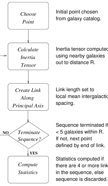
Figure 1:

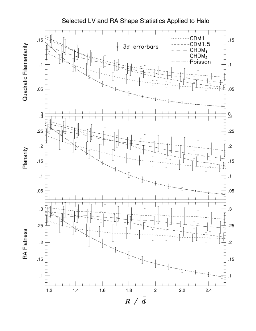
Figure 3: Halo Catalogs LV & RA Stats

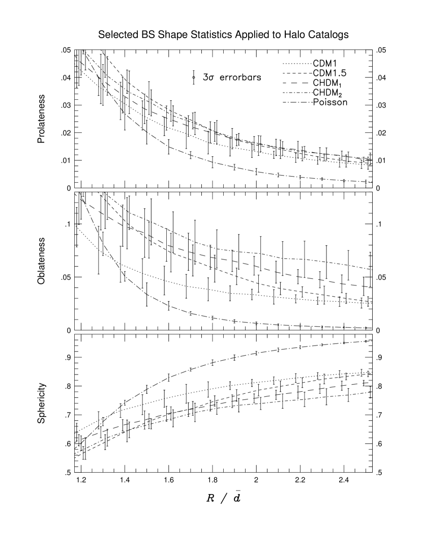
Figure 4: Halo Catalogs BS Stats

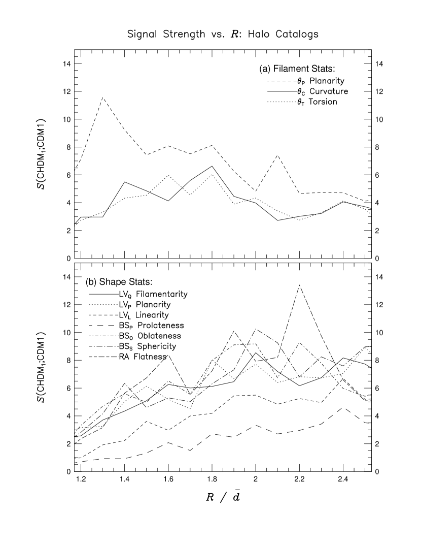
Figure 5: Signal strength for statistics applied to halo catalogs after breakup

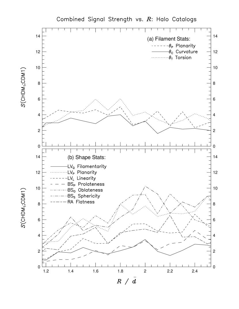
Figure 6: Combined signal strength for the halo catalogs

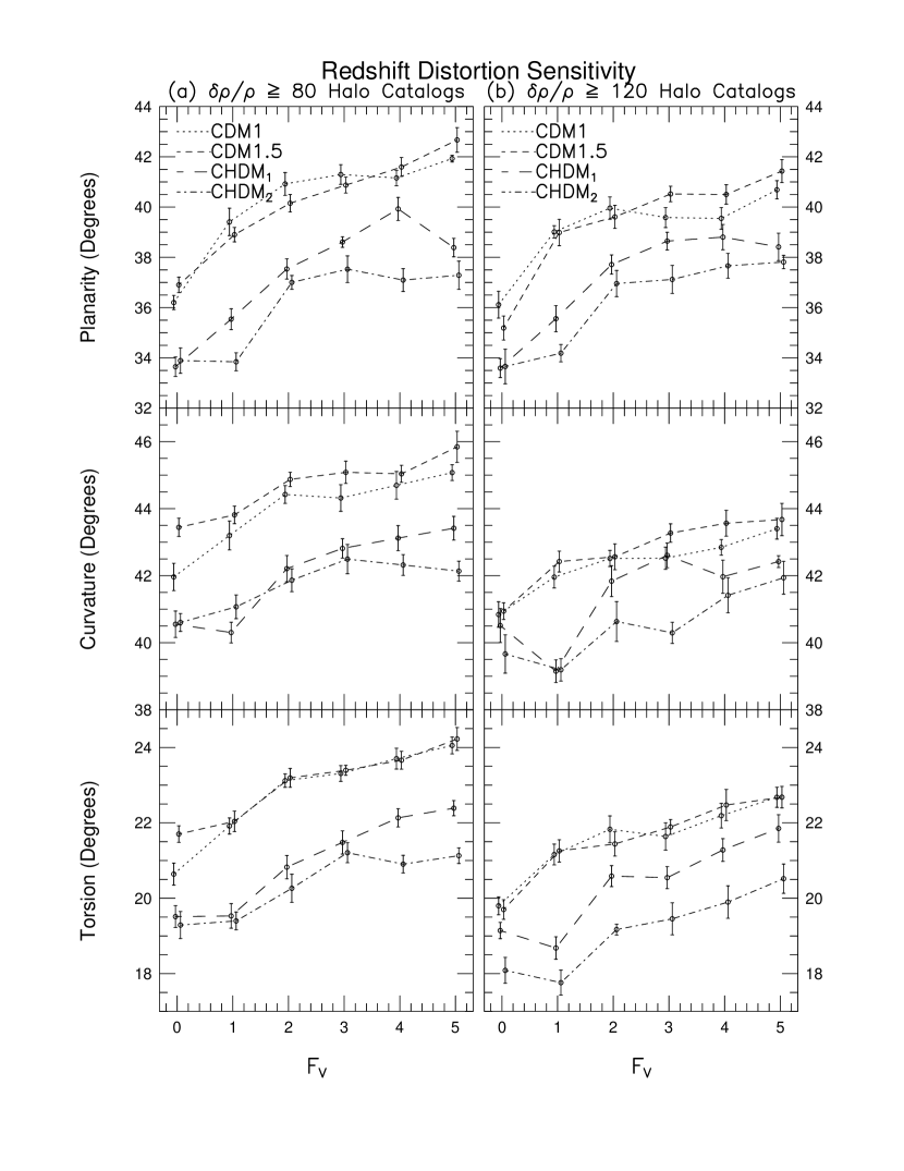
Figure 7: Redshift distortion test – Filament statistics

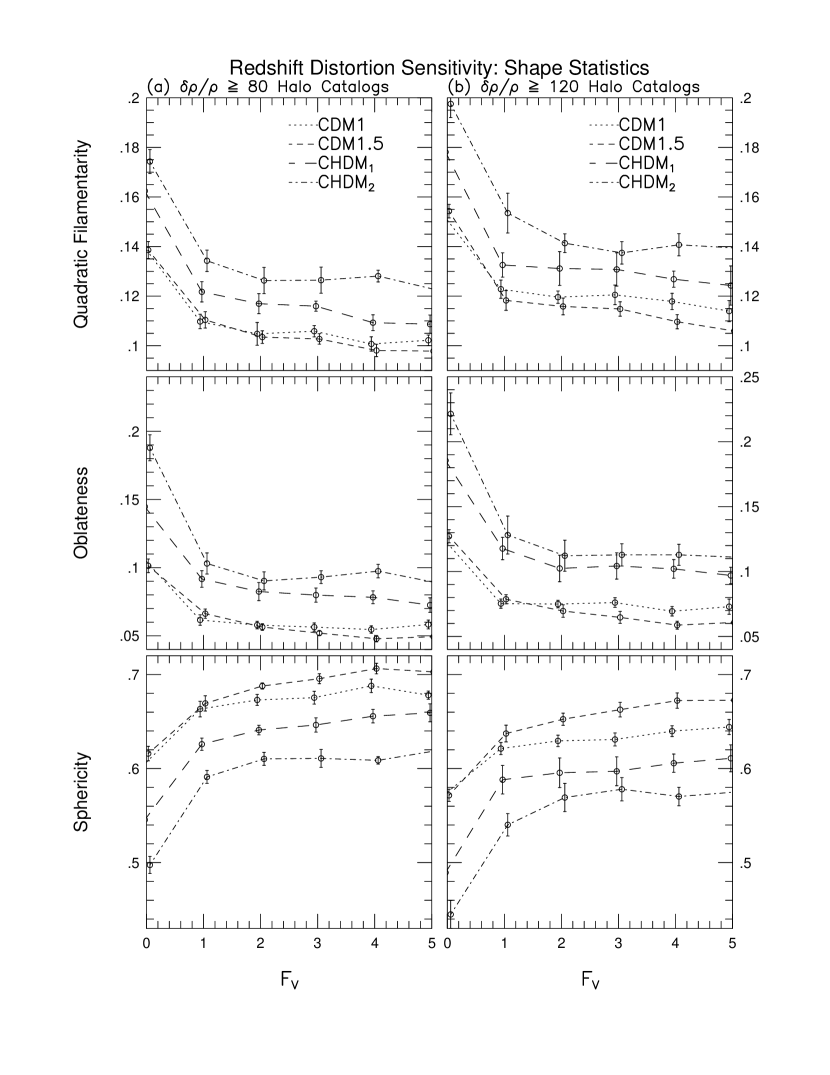
Figure 8: Redshift distortion test – Shape statistics

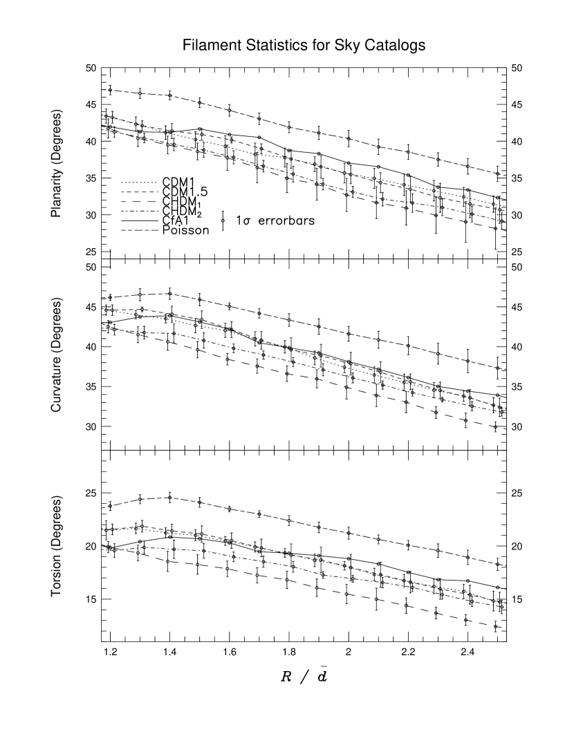
Figure 9: Sky Catalog Filament Stats

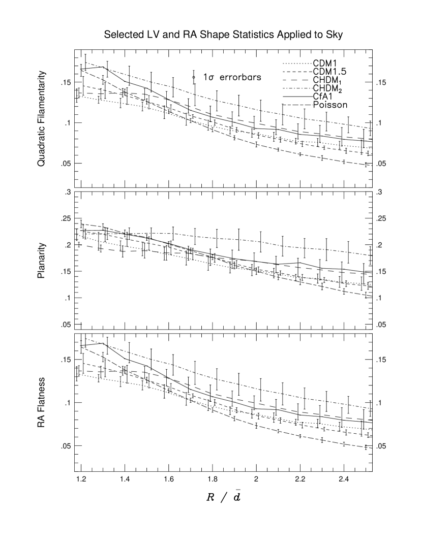
Figure 10: Sky Catalog LV & RA Stats

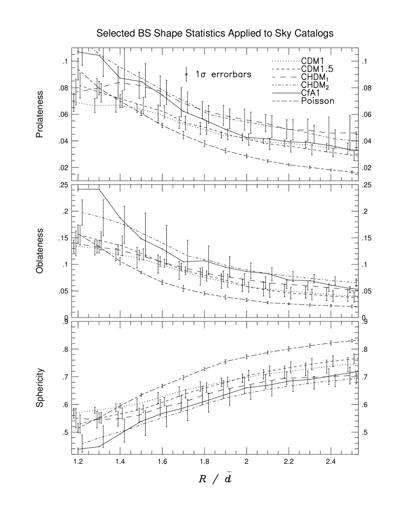
Figure 11: Sky Catalog BS Stats

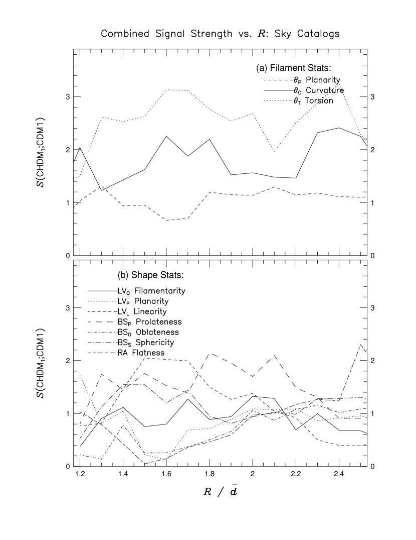
Figure 12: Combined signal strength for the sky catalogs

References

- [BS1992] Babul, A. & Starkman, G. 1992, ApJ, 401, 28
- [Baugh & Efstathiou1993] Baugh, C.M. & Efstathiou G. 1993, MNRAS, 267, 323
- [BHNPK1995] Brodbeck, D., Hellinger, D., Nolthenius, R., Primack, J.P., & Klypin, A.A. 1996, ApJ, in press [BHNPK]
- [CDP1996] Coles, P., Davies, A. & Pearson, R.C 1996, MNRAS, in press, astroph/9603139
- [Dekel1984] Dekel, A., 1984, in Domokos G., Kovesi-Domokos S., eds, Proc. Johns Hopkins Workshop 8, Particles and Gravity, Singapore: World Scientific, p. 206
- [deLapperant et al. 1988] deLapperant, V., Geller, M.J. & Huchra, J.P. 1988, ApJ, 332, 44
- [Gelb & Bertschinger1994] Gelb, J., & Bertschinger, E. 1994, ApJ, 436, 467
- [Geller1989] Geller, M.J. and Huchra, J.P. 1989, Science, 246, 897
- [Ghigna et al. 1994] Ghigna, S., Borgani, S., Bonometto, S., Guzzo, L., Klypin, A., Primack, J.R., Giovanelli, R. & Haynes, M. 1994, ApJ, 437, L71
- [Ghigna et al. 1995] Ghigna, S., Borgani, S., Tucci, M., Bonometto, S., Klypin, A., Primack, J.R. 1996, submitted to MNRAS
- [Hellinger1995] Hellinger, D. 1995, Ph.D. Thesis, Univ. of California, Santa Cruz
- [Katz & White1993] Katz, N., & White, S. D. M. 1993, ApJ, 412, 455
- [Kauffmann et al. 1995] Kauffmann, G., Nusser, A. & Steinmetz, M. 1995, MNRAS, submitted, astroph/9512009
- [Kerscher et al. 1995] Kerscher, M., Schmalzing, J., Retzlaff, J., Borgani, S., Buchert, T., Göttlober, S., Müller, V., Plionis, M. & Wagner, H. 1996, MNRAS, submitted, astroph/9606133
- [Klypin et al. 1993] Klypin, A.A., Holtzman, J.A., Primack, J.R., & Regos, E. 1993, ApJ, 416, 1
- [Klypin et al. 1996] Klypin, A.A., Nolthenius, R., & Primack, J.R. 1995, ApJ, in press [KNP96]
- [Klypin et al. 1996] Klypin, A., Primack, J.R. & Holtzman, J. 1996, in preparation
- [Luo & Vishniac1995] Luo, S. & Vishniac, E. 1995, ApJ Supp, 96, 429
- [Melott1990] Melott, A.L. 1990, Phys. Rep., 193, 1
- [Mecke et al. 1994] Mecke, K.R., Buchert, T. & Wagner, H. 1994, Astron. & Astrophys., 288, 697
- [Nolthenius et al. 1994] Nolthenius, R., Klypin, A.A. & Primack, J.R. 1994, ApJ, 422, L45 [NKP94]
- [Nolthenius et al. 1996] Nolthenius, R., Klypin, A.A. & Primack, J.R. 1996, ApJ, in press [NKP96]
- [Pearson & Coles1995] Pearson, R.C. & Coles, P. 1995, MNRAS, 272, 231
- [Primack1995] Primack, J.R. 1995, in S. Maurogordato, C. Balkowski, C. Tao & J. Tran Thanh, eds, Proceedings of the XXX Recontres de Moriond: Clustering in the Universe, Editions Frontieres, p. 184
- [Primack et al. 1995] Primack, J.R., Holtzman, J., Klypin, A., and Caldwell, D., 1995, Phys Rev Letters, 74, 2160
- [Santiago et al. 1995] Santiago, B., Strauss, M.A., Lahav, O., Davis, M., Dressler, A. & Huchra, J. 1995, ApJ, 446, 457
- [Santiago et al. 1996] Santiago, B., Strauss, M.A., Lahav, O., Davis, M., Dressler, A. & Huchra, J. 1996, ApJ, 461, 38
- [Sathyaprakash1996] Sathyaprakash, B.S, Sahni, V. & Shandarin, S.F. 1996, ApJ Lett, 462, L5
- [Somerville et al. 1996] Somerville, R., et al. 1996, in preparation
- [Van de Weygaert1991] Van de Weygaert, R., 1991, Ph.D. Thesis, Leiden Univ.
- [Vishniac1986] Vishniac, E. 1986 in Kolb, E.W., Turner, M.S., Lindley, D., Olive, K., Seckel, D., eds, Inner Space/Outer Space: The Interface Between Cosmology and Particle Physics, Chicago: Univ. of Chicago Press, p 190
- [Vogeley et al. 1991] Vogeley, M.S., Geller, M.J. & Huchra, J.P. 1991, ApJ, 382, 44
- [Vogeley et al. 1992] Vogeley, M.S., Park, C., Geller, M.J. & Huchra, J.P. 1992, ApJ, 391, L5