Composition Mixing during Blue Straggler Formation and Evolution

Abstract

We use smoothed-particle hydrodynamics to examine differences between direct collisions of single stars and binary star mergers in their roles as possible blue straggler star formation mechanisms. From our simulations we find in all cases that core helium in the progenitor stars is largely retained in the core of the remnant, almost independent of the type of interaction or the central concentration of the progenitor stars.

We have also modelled the subsequent evolution of the hydrostatic remnants, including mass loss and energy input from the hydrodynamical interaction. The combination of the hydrodynamical and hydrostatic models enables us to predict that little mixing will occur during the merger of two globular cluster stars of equal mass. Unmixed and completely mixed models can both explain the luminosities of the brightest BSSs by the merger of two turnoff mass stars. In contrast to the results of Proctor Sills, Bailyn, & Demarque (1995), we find that neither completely mixed nor unmixed models can match the absolute colors of observed blue stragglers in NGC 6397 at all luminosity levels. We also find that the color distribution is probably the crucial test for explanations of BSS formation — if stellar collisions or mergers are the correct mechanisms, a large fraction of the lifetime of the straggler must be spent away from the main sequence. This constraint appears to rule out the possibility of completely mixed models. For NGC 6397, unmixed models predict blue straggler lifetimes ranging from about 0.1 to 4 Gyr, while completely mixed models predict a range from about 0.6 to 4 Gyr.

1 Introduction

Blue straggler stars (BSSs) are objects in open and globular clusters that are brighter and bluer than the cluster main-sequence turnoff (MSTO), appearing to follow an extension of the main sequence. Over the years a number of explanations for their existence have been considered, including an extended period of star formation in the cluster, prolonged main-sequence lifetimes for some cluster stars as a result of mixing, and the formation of objects more massive than the current-day MSTO via the merger of close binary stars or through the direct collision of two or more stars (see Stryker 1993 and Bailyn 1995 for recent reviews).

With the discovery of eclipsing contact, semi-detached and detached binaries among the BSS or main-sequence stars in several globular clusters (Niss, J$\o$rgensen, & Lausten 1978; Mateo et al. 1990; Hodder et al. 1992; Kaluzny & Krzeminski 1993; Yan & Mateo 1994; Rubenstein & Bailyn 1996; Yan & Reid 1996) and the discovery of populations of bright BSS near the cores of very dense clusters (e.g. Aurière, Ortolani, & Lauzeral 1990; Paresce et al. 1991, Lauzeral et al. 1992; Auriere et al. 1990; Yanny et al. 1994a,b), there is growing consensus that most BSS in globular clusters are in mass-transfer binary systems or are the remnants of stellar collisions. We will refer to these two possibilities as “binary merging” and “collisional merging” respectively.

If these two processes are the main mechanisms for BSS production, then BSSs become interesting in a broader context than as footnotes to our understanding of stellar evolution. The binding energy in primoridal binary systems has long been invoked as a source of energy in globulars to prevent or halt core collapse and/or provide the energy for post-core-collapse expansion (e.g. Hut et al., 1992). If signatures of binary mergers could be recognized and the numbers and lifetimes of the remnants accurately determined, it would be possible to place observational constraints on the input energy of binary “burning”. Similarly, if the remnants of star-star, binary-star and binary-binary interactions could be unambiguously identified and the lifetimes of the remnants calculated, then observations of these objects in clusters with different stellar densities and velocity dispersions would give observational constraints on the stellar cross-sections for interaction.

Bailyn (1992) suggested that BSSs formed during binary mergers could be distinguished from collisional remnants by differences in photometric properties. Based on the Benz & Hills (1987) hydrodynamical calculations of colliding stars, Bailyn assumed that the remnants of collisional mergers would be effectively fully mixed, with larger helium envelope contents than the progenitor stars or than the remnant of a binary merger of comparable total mass. BSSs formed in collisional mergers would therefore be bluer than the extension of the cluster main sequence, and BSSs formed in binary mergers would tend to be redder – these remnants look like evolved versions of higher-mass (than either of the original binary components) stars. For a given total mass, collisional remnants would also be more luminous than binary merger remnants. Bailyn & Pinsonneault (1995) suggested that the composition profile differences between BSSs formed by the two processes would also lead to different lifetimes and evolutionary tracks in the color-magnitude diagram. This would lead to different luminosity functions for populations of BSSs formed via the two paths. Specifically, BSSs created via binary merger would be seen less often at the bright end of the luminosity function as the higher core helium content reduces the main sequence lifetime of these stars compared to BSSs created by stellar collisions.

The observational data appear to support the idea of BSS formation via the two mechanisms and implicitly support the difference in composition profiles of the two different types of remnants. Bailyn & Pinsonneault (1995) interpret the BSS luminosity function of 47 Tucanae (NGC 104) as being consistent with production via collisions of single stars. The brightest BSS appear to form a separate class in several other globular clusters. In M3 (NGC 5272), the BSSs exhibit a gap in their radial distribution (Ferraro et al. 1993), and the innermost BSSs have a different luminosity function from the outer group (Bailyn & Pinsonneault 1995), consistent with a collisional origin in the center and binary origin in the outskirts. In the low-density cluster NGC 5053, the 12 brightest BSSs are more centrally concentrated than the 12 faintest (Nemec & Cohen 1989). The post-core-collapse globular cluster NGC 6397 sports seven BSSs that are significantly brighter than the rest of the known BSSs (Lauzeral et al. 1992; Rubenstein & Bailyn 1996). Because the bright BSS population in NGC 6397 shows very clear differences from the faint population in magnitude and in physical location in the cluster (6 out of 8 of the BSSs within $15^{\prime\prime}$ of the core are bright; Lauzeral et al. 1992), it is an ideal test of formation mechanisms for the most massive BSSs. Proctor Sills, Bailyn & Demarque (1995) interpret these stars as being the results of stellar collisions during which the remnants are fully mixed, based solely on the agreement in color with stellar evolution models. Although one W UMa contact binary has been identified outside the core, none of the observed BSSs (which include the core BSSs) show variability (Rubenstein & Bailyn 1996). This provides weak support for the collision hypothesis.

For interpreting these observations, the question of whether or not BSSs are chemically mixed during their formation is therefore a key one. Many studies have followed the hydrodynamics of stellar interactions, partly in an attempt to understand possible BSS creation mechanisms. Benz & Hills (1987, 1992) carried out smoothed-particle hydrodynamics (SPH) simulations of collisions of equal and unequal mass polytropes of index $n=3/2$. In their simulations, they looked at particle mixing at low resolution, dividing the progenitor stars into four equal mass bins at four radial positions, and examined the positions of the particles in the remnant. They found that head-on collisions mixed the material less than did grazing impacts (which result in maximum mass loss). So, if two turnoff-mass stars (with significant helium in their cores due to nuclear processing) collided, the core helium would be more highly mixed throughout the remnant in a grazing collision than in a head-on collision. Similarly, for unequal mass collisions, Benz & Hills found that the more massive star in the collision was thoroughly mixed, and that the less-massive star settled to the core of the more massive. Both results would imply a larger envelope helium abundance, and a mixing of hydrogen into the core of the remnant, indicating that BSSs evolve off of the main sequence in a nuclear timescale.

Although the Benz & Hills work has been widely used to interpret BSSs, it is not clear that their models are entirely appropriate. For BSSs to be created above the level of the MSTO, they must be drawn from stars near the turnoff mass. MSTO stars have high density contrast (the ratio of central density to average density), and so are better modelled by polytropes of index higher than $n=3/2$. Lombardi, Rasio, & Shapiro (1995) presented results for grazing collisions of equal-mass $n=3$ polytropes (with a polytropic equation of state having $\Gamma=5/3$ to best model the gas behavior). If the progenitor stars have composition profiles like those of turnoff stars, the resulting remnant has a helium profile as a function of $m/M_{tot}$ that is essentially identical to the progenitors. Thus, the higher density (and gravity) of the stellar cores protects them against mixing until they are able to merge. The higher core helium abundance then implies that the remnant BSS would have a core hydrogen-burning lifetime that is much shorter than the main sequence lifetime of a zero-age star of equal mass.

There is another potential source of mixing that could significantly influence the magnitude and color of a blue straggler. As Leonard & Livio (1995) theorize, the energy that is input into the envelope of the remnant of a collisional or binary merger can cause the star to swell to pre-main sequence proportions, which results in large-scale convective mixing. The major questions in this case are: how much energy is needed to induce the star to mix completely, and can typical stellar interactions in globular clusters provide enough energy?

In this paper, we attempt to model the entire merger process in detail. We present hydrodynamical simulations using both $n=3/2$ and $n=3$ polytropes in head-on collisions, grazing collisions, binary collisions, and binary mergers in order to examine the effects of the character of the stellar interaction on hydrodynamical mixing. We use this information to create one-dimensional stellar models that incorporate the mixing and energy inputs derived from the hydrodynamical simulations, so that we can also determine the effects of convective mixing. Throughout, we will concentrate on equal-mass star collisions, which are particularly relevant to modelling the brightest BSSs. In §2, we discuss details of the hydrodynamic and hydrostatic calculations for the collisional and binary merger mechanisms. In §3 we present the results of these calculations: the helium profiles and the evolutionary paths of the remnants after the interaction. In §4 we look into the observational implications of our calculations, and consider the evidence for these methods of creating blue stragglers.

2 Calculations

2.1 Hydrodynamics Simulations

We have modelled various kinds of stellar interactions using smoothed particle hydrodynamics, in particular utilizing the TREESPH code (Hernquist & Katz 1989). Our computations follow those of Goodman & Hernquist (1991), with slight differences. We refer the reader to these references for details of the operation of the code. Here we provide a short summary of points that will be needed in other parts of the paper.

The hydrodynamical calculations reported in this paper all involve progenitor stars modelled as polytropes of index $n=3/2$ or $n=3$. For the $n=3/2$ simulations carried out in the first phase of this study, we chose to integrate the entropy equation. For a pure polytrope, the specific entropy of any two parcels of gas are identical, making it straightforward to set up the initial model. For $n=3/2$, we are immediately given a realistic adiabatic index for the gas of $\Gamma=5/3$. However, for $n=3$ polytropes with $\Gamma=5/3$, it is more convenient to create the initial model by adjusting the energies of the initial particles (Lai, Rasio, & Shapiro 1993), and to use the thermal energy equation to evolve the particles. We have followed this procedure for our $n=3$ runs.

We have chosen not to model changes in the equation of state in the stars resulting from composition changes. To first order this can be accounted for using polytropes of higher index for stars that have more core helium. The higher molecular weight of helium compared to hydrogen reduces the pressure that can be exerted by the gas, resulting in a more centrally concentrated structure.

For all of our two-star collisions, we used 3000 SPH particles in each star. For the Goodman & Hernquist (1991) four-star interactions we have analyzed, 2048 particles were used in each star. A spherically symmetric spline kernel (Monaghan & Lattanzio 1985) was used to smooth each particle (the density goes to zero at a distance $2h$ from the particle center, where $h$ is the smoothing length). The smoothing length of each particle was allowed to vary adaptively with time in order to ensure interaction with only the $N_{s}$ nearest neighbors (we chose $N_{s}=38$).

We have used an artificial viscosity of the form (Monaghan 1992):

$${\bf a}_{i}^{visc}=-\sum_{j}m_{j}\Pi_{ij}\frac{1}{2}\left[\nabla_{i}W({\bf r}_{i}-{\bf r}_{j},h_{j})+\nabla_{i}W({\bf r}_{i}-{\bf r}_{j},h_{i})\right],$$

where

$$\Pi_{ij}=\frac{-\alpha\mu_{ij}\overline{c}_{ij}+\beta\mu_{ij}^{2}}{\overline{\rho}_{ij}},$$

and

$$\mu_{ij}=\left\{\begin{array}[]{ll}\frac{{\bf v}_{ij}\cdot{\bf r}_{ij}}{h_{ij}(r_{ij}^{2}/h_{ij}^{2}+\eta^{2})}&\mbox{for}\>{\bf v}_{ij}\cdot{\bf r}_{ij}<0,\\ 0&\mbox{for}\>{\bf v}_{ij}\cdot{\bf r}_{ij}\geq 0.\end{array}\right.$$

Also, $r_{ij}=\left|{\bf r}_{i}-{\bf r}_{j}\right|$, ${\bf v}_{ij}={\bf v}_{i}-{\bf v}_{j}$, $\overline{c}_{ij}=(c_{i}+c_{j})/2$ (the average sound speed for two particles), $h_{ij}=(h_{i}+h_{j})/2$, and $\overline{\rho}_{ij}=(\rho_{i}+\rho_{j})/2$. Here we have used $\alpha=0.5,\beta=1.0$, and $\eta^{2}=0.01$.

For the majority of our initial polytrope models, the particles were distributed randomly in the star’s volume, and were given masses proportional to the density of the appropriate polytrope. (For runs that used equal-mass particles, the positions of the particles were weighted according to the local density of the polytrope.) A star created in this way is prone to oscillations because of small irregularities in the sampling of the gas volume. We allowed the star to adjust by introducing frictional damping for a short period of time.

Our simulations of single star interactions generally fell into one of three categories: (1) binary merger (BM) — the two stars were placed on circular orbits with synchronous rotation in order to simulate a tidally-locked binary; (2) head-on collision (HC) — the two stars were given velocities in the center-of-mass frame that caused them to collide with zero impact parameter; (3) grazing collision (GC) — the two stars were given velocities that caused them to collide with an impact parameter $0<R_{min}/(R_{1}+R_{2})<1$, where $R_{1}$ and $R_{2}$ are the initial radii of the two stars. Because we are only interested in interactions typical of globular clusters, we have in all HCs and GCs used $V_{\infty}=0$, where $V_{\infty}$ is the relative velocity in the center-of-mass frame at infinite separation. In addition, the stars in HCs and GCs were given initial separations of $5(R_{1}+R_{2})$ in order to strike a compromise between computational time and the initial gravitational perturbations on the input stars. For the BMs of $n=3/2$ polytropes, we started the stars with a separation $a=1.3(R_{1}+R_{2})$, and for the $n=3$ polytropes, the separation was $a=1.1(R_{1}+R_{2})$. These separations were large enough that the stars were able to fully relax in the mutual potential before merging occurred.

The interactions were followed until a relaxed remnant was formed in each case. This was judged by the lack of variation of the total internal and gravitational energies with time during each run. In this way we hope to have adequately modeled the hydrodynamical mixing that occurs during the formation of the remnants. For HCs, the remnants were nearly quiescent — approximately spherical with extremely low particle kinetic energies. For GCs and BMs though, the input angular momentum typically created a remnant that was oblate, and in some cases also had a disk of material. The spin-down timescale for these kinds of remnants was too long to be modeled further by hydrodynamical means. To determine the final mass of these remnants, we followed the algorithm of Benz & Hills (1987), and examined each particle to see if it had enough energy to escape. This was judged to be true if $E>0$ for the particle, where

$$E=E_{K}+P/(\Gamma-1)+\rho\Phi,$$

where P is the pressure on the particle, $\rho$ is particle density, $\Phi$ is the particle’s gravitational potential, and

$$E_{K}=\left\{\begin{array}[]{ll}0&\mbox{if}\>xv_{x},\;yv_{y},\;\mbox{or}\>zv_{z}<0,\\ \frac{1}{2}\rho\left[v_{x}^{2}+v_{y}^{2}+v_{z}^{2}\right]&\mbox{otherwise}\end{array}\right.$$

is the outgoing kinetic energy.

We note that our BM run with polytropes of index $n=3$ would not have merged on a timescale that it was possible to model. Once started, the binary immediately formed a common envelope configuration that lost energy at a very low rate even though the stars were started with a small initial separation. This shows that dynamical instabilities in synchronized binaries of the type discussed by Rasio & Shapiro (1995) occur for much smaller separations in $n=3$ polytropes than they do for $n=3/2$ (if they occur at all), or the timescale for the instability is longer than we could reasonably simulate. We ended up having to force the merger to occur by applying a small amount of friction to the orbital motions. The density contours for the common-envelope binary are shown in Figure 1 before friction was applied. This run should be regarded as somewhat suspect because physical processes like convection could have time to occur if the merger timescale is long enough.

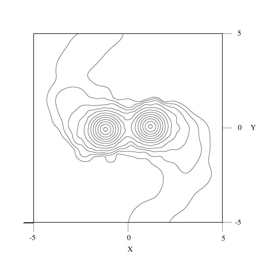
Figure 1: Density contours for the binary merger of two $n=3$ polytropes. This represents the gas configuration before friction was applied. The contours are evenly spaced two per decade, and range from densities (in the orbital plane of the binary) of $10^{-5}$ g/cm³ to 10 g/cm³.

2.2 Hydrostatic Evolution Calculations

To follow the subsequent phase of quiescent stellar evolution, we carried out a number of one-dimensional stellar evolution calculations. In order to create a realistic initial model, the helium distribution in the remnant from the hydrodynamical calculations had to be determined, and projected into a radial profile. To accomplish this (for remnants that were oblate, or had disks), we calculated the moment of inertia tensor for the particles bound to the remnant. The remnants always had a high degree of rotational symmetry, so we used the angular momentum vector to define the minor axis. The moments of inertia about the three principal axes were then used to calculate the oblateness of the remnant. For axis lengths $a\geq b\geq c$ (and moments of inertia $I_{3}\leq I_{2}\leq I_{1}$), the oblateness of the remnant was characterized by

$$\frac{a}{c}\simeq\frac{a+b}{2c}=\frac{\sqrt{I_{1}-I_{2}+I_{3}}+\sqrt{I_{1}+I_{2}-I_{3}}}{2\sqrt{-I_{1}+I_{2}+I_{3}}}.$$

The oblateness was typically computed for a small radial range near the center of mass of the remnant, because there were definite changes as a function of radius. It was most important to get the average oblateness of the core of the remnant to ensure that the helium profile there was computed as accurately as possible. Once this was done, the corrected radius of each particle was calculated, and the particle’s mass was put into bins. The helium profile calculated from this procedure was then mapped onto a pre-existing one-dimensional stellar model. To test the extreme case of complete mixing in BSSs, we computed the average helium mass fraction from helium profiles derived in our SPH simulations, and then imprinted the average helium abundance throughout.

These calculations were made with a version of the Eggleton stellar evolution code (Eggleton 1991). The Eggleton code utilizes an adaptive mesh, which is adjusted to put points where variations in mass, temperature, and pressure are the largest. In our calculations, we have followed the evolution of only ¹H, ⁴He, ¹²C, and ¹⁶O, as the error in the helium abundance introduced by the small reaction network is easily dwarfed by uncertainties in the hydrodynamical mixing, as we will discuss later.

We use the equation of state of Eggleton, Faulkner & Flannery (1973). More importantly, we use opacities for $\alpha$-enhanced compositions calculated by the OPAL group (Rogers 1996; see Iglesias, Rogers & Wilson 1992 for a description of the physics). We have chosen to use the most up-to-date opacities that are available because they are known to primarily affect the color of a star, which will be important later in comparisons with observational data. For low temperature opacities, we have used the tables of Weiss, Keady, & Magee (1990). This choice is not particularly important because surface temperatures for blue stragglers near the MS are higher than the low temperature edge of the OPAL tables. As a result, the position of our models in the HR diagram during the blue straggler phase will not be affected.

An $\alpha$-element enhancement of $+0.3$ dex was also included as globular clusters are known to have composition enhancements of this order (Pilachowski, Olszewski & Odell 1983; Gratton, Quarta & Ortolani 1986). These enhancements were taken into account explicitly in the ¹⁶O abundances in the reaction network and in the OPAL opacities. Model luminosities and effective temperatures were converted to the observational plane via bolometric corrections and color transformations from VandenBerg (1992). Table 1 lists data for evolutionary runs from the main sequence for these runs.

As suggested by Leonard & Livio (1995), the kinetic energy of the stellar interaction can be converted into thermal energy, causing the remnant to swell like a pre-main sequence star, potentially inducing convective mixing in the remnant. To test this hypothesis, we have computed models that start from a pre-main sequence configuration. This has been accomplished by turning off convective mixing of composition, and then gradually increasing the magnitude of a constant energy generation (per unit mass) term for each model zone until the star was placed well onto the Hayashi track. The constant energy generation term could then be turned off, allowing the star to contract back toward the main sequence on a thermal timescale.

We do not attempt to model the evolution of the remnant between the end of the SPH calculation and the beginning of this “pre-main sequence phase”. However, we believe that the details of this adjustment are not particularly important. First, any convective mixing will occur on timescales shorter than the thermal adjustment timescale. As such, if convective mixing occurs before the remnant becomes hydrostatic, it will almost certainly be convective to about the same extent at the beginning of the pre-main-sequence-like phase. Mass loss or angular momentum loss from the remnant could affect this argument, but we will examine it again in § 4.1. Second, as we will see later, for typical BSS masses, convection actually tends to be suppressed by the energy added during the collision. No energy input was applied to the completely-mixed models, as the thermal relaxation timescale is short compared to the nuclear evolution timescale, so that the energy input would not significantly change the expected BSS lifetime.

3 Results

Table 2 summarizes the SPH calculations that we have made or reanalyzed. Column (2) gives the mass of the most massive remnant in each interaction in units of the initial star mass. Column (3) gives the oblateness of the core of the remnant (taken to be any particles with a deprojected radius $r<0.5$ in units of the initial star radius). Columns (4) – (6) give the kinetic, internal and gravitational energies of the particles bound to the remnant (in units of $GM^{2}/R$, where $M$ and $R$ refer to the input stars). The table also lists energy values for polytropes having $\Gamma=5/3$. Finally, column (7) gives the helium mass fraction at the center of the remnant, assuming that the progenitor stars both had helium profiles matching that of a star at the turnoff ($0.794M_{\odot}$).

We have re-examined data from Goodman & Hernquist (1991) for collisions between equal-mass binary stars. These simulations involved polytropes of index $n=3/2$ with equal separations $a$, placed on parabolic orbits which brought them to pericenter separations between 0 and $3a$. Each star had a smaller number of particles than the ones in our two-star collisions, but tests indicate that this has little effect on the calculated helium profile. These simulations should be useful for checking the effects of multiple mergers, and for examining the differences introduced by the altered kinematics of the interaction. Runs 22 and 43 from Goodman & Hernquist have been omitted from consideration because one star involved in the merger had not completely merged into the remnant by the end of the simulation. As a result, a bump appears in the helium profile away from the core.

We have performed other simulations to test the effects of our parameter choices in the SPH formalism. One such comparison can be seen in the runs HCQ1 and HCQ1BH for $n=3/2$. These simulations tested the sensitivity of our choices relative to those of Benz & Hills (1987) — specifically with respect to the form of the artificial viscosity and the smoothing length for particles. With constant smoothing lengths $h$ (in time) and $\beta=0$ in the artificial viscosity, we have been able to essentially reproduce the energy evolution of Benz & Hills’s $R_{min}/(R_{1}+R_{2})=0.0$ and $V/V_{esc}=0.0$ run. We believe the form of the artificial viscosity we use is more realistic (Hernquist & Katz 1989), but it makes fairly little difference. We do find more mixing of hydrogen into the core, and more energy input into the remnant’s envelope.

Modeling of $n=3$ polytropes is difficult due to the large density contrast between core and surface. As a result, we have completed runs (HCQ1 and HCQ1EM) that test the effect of resolution on hydrodynamical mixing and envelope energy input. In run HCQ1, the SPH particles were given masses proportional to the density at their positions in the input stars. In run HCQ1EM, all particles had equal mass, giving us improved resolution of the core regions at the expense of less accurate modeling of the outer envelope. The amount of mixing is found to be larger in the HCQ1 run, and appears to be due to a small number of massive (helium-rich) core particles in the initial stars being pushed away from the core. The envelope energy input is also slightly higher in the HCQ1 run, which is probably due to the improved treatment of the initial contact between the two stars. We conclude that our use of unequal mass particles probably means that our estimates of envelope energy input are accurate, while our estimates of hydrodynamical mixing are overestimated (see Lombardi, Rasio, & Shapiro 1995 for a short discussion).

Figures 2 and 3 show the helium profiles derived from the simulations. The input stars were given helium profiles corresponding to a star near the cluster turnoff ($0.79M_{\odot}$) for a star with $Z=0.00041$ (corresponding to an $\alpha$-enhanced composition of [Fe/H] $=-1.91$) and $Y=0.235$. We will discuss this choice of composition in §4.2.

Figure 2: Helium profiles for two-star mergers. The solid line indicates the profile for the initial stars, the short dash lines show the profiles for the most- and least-mixed of the mergers during binary encounters (runs 54 and 57 respectively from Goodman & Hernquist 1991), the long dash line is an $n=\frac{3}{2}$ binary merger, and the dotted line is an $n=\frac{3}{2}$ head-on collision, and the dot-dashed line is an $n=3$ grazing collision (the $n=3$ head-on collision is virtually identical).

Figure 3: Helium profiles for three-star mergers. The two profiles shown are from simulations in Goodman & Hernquist (1991): run 6 (dotted line), and run 49 (dashed line).

Table 3 presents the results of the hydrostatic evolution for the blue straggler models. Figure 4 shows a comparison of some typical evolutionary tracks for our BSS models in the HR diagram. We find that the relaxation phase essentially follows the post-main sequence track to the point where the remnant restarts stable burning of its remaining core hydrogen. This is reasonable, given the similarity of pre-main sequence and post-main sequence tracks near the zero-age main sequence. This implies that collision or merger remnants that are relaxing back to a hydrostatic configuration would be indistinguishable from hydrostatic blue stragglers based on photometry alone. However, the relaxation phase is short compared to the hydrogen-burning stage.

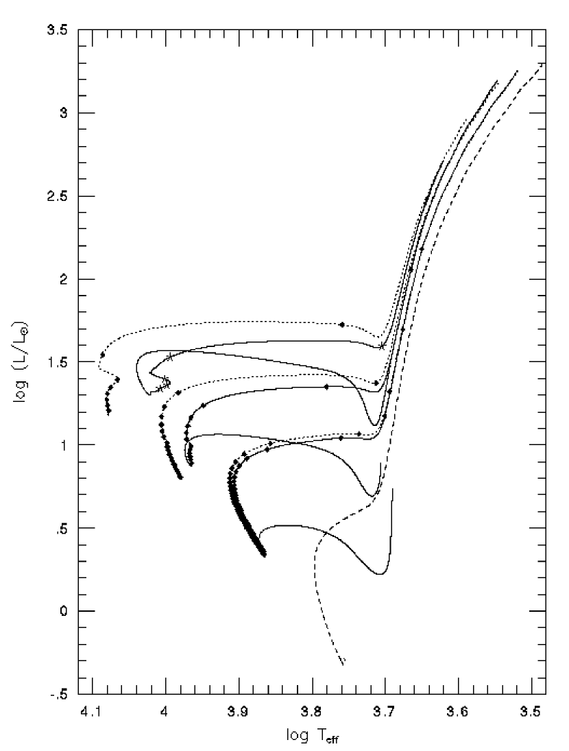
Figure 4: HR diagram comparing our mixed (dotted lines) and unmixed (solid lines) BSS models for masses of 1.47, 1.30, and 1.07 $M_{\odot}$ from most luminous to least luminous. Symbols on the evolutionary tracks indicate time intervals of $5\times 10^{7}$ yr for the 1.47 $M_{\odot}$ unmixed model (five-point stars), and $10^{8}$ yr for all other models (filled circles). A 0.79 $M_{\odot}$ track is also included (dashed line), which has an age of 14 Gyr at its turnoff from the main sequence.

The larger the amount of hydrogen remaining in the core, the higher the luminosity at which a hydrostatic structure is re-established on the evolutionary track. Based on our models, which predict little mixing, we find that the majority of the early (long) MS phase is avoided, considerably shortening the life of the BSS.

4 Discussion

4.1 Model Analysis and Fits

4.1.1 Helium Profiles

From the helium profiles shown in Figure 2, it appears that there is slightly more mixing in mergers involving $n=3/2$ polytropes than in $n=3$ polytropes in general. However, in every one of our SPH simulations, we find that high helium abundances in the cores of the progenitors are preserved during the interaction. This result is in agreement with the simulation of an $n=3$ GC by Lombardi, Rasio, & Shapiro (1995). Our result is, however, in contradiction to the “maximum mass-loss” simulation of Benz & Hills (1987) — an $n=3/2$ GC. The histogram they present indicates much greater mixing of helium-rich core material into the envelope.

Our simulations also show that the remnants of head-on collisions are among the least-mixed of the runs. Grazing collisions and binary mergers have slightly larger amounts of mixing, but have profiles that are qualitatively similar to each other. As a result, the remnants of grazing collisions and binary mergers should evolve in nearly identical ways. If we are to judge from the hydrodynamical mixing alone, neither fully-convective ($n\approx 3/2$; $M\leq 0.4M_{\odot}$) nor radiative ($n\approx 3$; $M\geq 1.0M_{\odot}$) globular cluster stars will completely mix during a typical encounter.

4.1.2 Convective Mixing

Leonard & Livio (1995) suggested that energy input from the interaction could drive an expansion of the remnant’s surface well beyond what would be expected for a passively evolving main-sequence star of the same mass. For a large enough expansion, the star is driven to the Hayashi track, where a surface convection zone develops that mixes much of the interior. If this convection zone is extensive enough, it could potentially mix core helium into the envelope. However, for the highest mass BSSs, a couple of factors work against convective mixing driven by this energy input.

First, energy input from the hydrodynamical interaction forces a temperature decrease in the core as the gas expands. As a result of the reduced core temperature, the core temperature gradient is lowered, which will completely quench core convection as long as thermal energy is being released by the bloated remnant. The more massive the remnant is, the hotter it is as a main-sequence star. Consequently, large energy inputs are necessary to force the star to expand to the point where a surface convection zone can move inward to reach helium-enriched layers. The reverse of this process occurs in the pre-main-sequence phase of evolution.

Second, we note that during pre-main-sequence contraction, it is the core of the star that becomes radiative first. This occurs when the central temperature is high enough that the matter is completely ionized, and the density is high enough that electron scattering is the dominant source of opacity. The resultant decrease in the total opacity allows radiation to efficiently carry thermal energy away from the core, eliminating the need for convection. A similar effect occurs for BSSs driven to the Hayashi track, but to a greater extent. Because of the high helium content of the core (mostly unaffected by the hydrodynamical part of the merger, and also untouched by core convection), the opacity is even lower than in a pre-main-sequence star for the same physical conditions ($\kappa\approx 0.20(1+X)\;\mbox{cm}^{2}/\mbox{g}$ for electron scattering in the Thomson limit). As a result, the higher core helium content can prevent a surface convection zone from penetrating into the core even on the Hayashi track if the remnant is massive enough.

The higher mass of the remnant also results in a different distribution of convective zones when it returns to the main sequence. For globular cluster ages of order 14 Gyr, turnoff stars have masses of approximately $0.8M_{\odot}$, with surface convection zones containing relatively little mass. However, main-sequence stars with mass greater than about $1M_{\odot}$ develop core convection, while the surface convection zone disappears. Although convective cores never achieve the extent necessary to completely mix the star in this range of masses, they can mix material into the core from regions that are richer in hydrogen. The higher the mass of the remnant, the larger the extent of the convective core when the remnant has re-established hydrogen burning via the CNO cycle. This effect can mix extra hydrogen into the core. We find that for our most massive model ($1.47M_{\odot}$), the core convection zone covers the innermost $0.2M_{\odot}$, and increases the core hydrogen mass fraction by about 0.1. In contrast, core convection enriches the core of our $1.30M_{\odot}$ model by only 0.02 (covering $0.07M_{\odot}$ of material), and core convection is never established in the $1.07M_{\odot}$ remnant.

There are undoubtedly errors in the total energies of the SPH runs of a few percent due to our use of adaptive smoothing lengths, and our use of entropy equation integrations in the $n=3/2$ runs (Hernquist 1993). However, the absolute accuracy of the total energies is not important for this study because of the large amount of energy necessary to drive the star back up the Hayashi track. The relatively small kinetic energies involved in collisions in globular clusters makes it unlikely that this energy input completely mixes the star except in the rarest of situations.

We have seen in the discussion so far that the remnant mass has a variety of implcations for the effectiveness of convection in the merger remnants. As a result, we expect that mass loss during the merger and later during spin-down will have some influence on the next stages of the remnant’s evolution. Hydrodynamical mass loss does not exceed about 7% in any of our simulations, which will not affect our conclusions. A merger can also produce a disk around the remnant, which could in turn be driven away via interaction with the central object and angular momentum transfer. However, disks are formed in few of the simulations, and even then the majority of the mass resides in the central object. So, we believe that mass loss during the merger process will not change our conclusions on the matter of mixing.

4.2 NGC 6397

NGC 6397 is one of the nearest globular clusters, and photometry of its BSSs has been carried out even into its dense core (Lauzeral et al. 1992; Rubenstein & Bailyn 1996). The core population of BSSs is significantly brighter than the majority of BSSs farther from the center. The high central density of the cluster may indicate that these stragglers are the result of stellar mergers. For these reasons, this cluster makes an excellent subject for comparison between our models and observations. Before proceeding with fits to the BSSs in NGC 6397, we briefly discuss the characteristics of the cluster that could influence the placement of the BSSs in a diagram of $M_{V}$ versus $(B-V)_{0}$.

We have chosen to use the Zinn & West (1984) metallicity [Fe/H] $=-1.91$. As summarized in Table 5 of that paper, the majority of other studies have found values slightly higher: [Fe/H] $\approx-1.8$. Some exceptions have been [Fe/H] $=-2.01$ (Smith 1984), $-2.24$ (Pilachowski 1984), and $-1.96$ (from one star; Lambert, McWilliam, & Smith 1992). Recently however, it has been found that the Zinn & West scale is decidedly nonlinear with respect to a consistently reduced set of high-dispersion spectroscopic determinations of cluster metallicities (Carretta & Gratton 1996b). If the Zinn & West value is corrected using the formula given by Carretta & Gratton, we derive [Fe/H] $=-1.69$. Carretta & Gratton (1996a) measure a value [Fe/H] $=-1.82\pm 0.04$. As a result we will consider the potential metallicity error to be $\pm 0.2$ dex, with somewhat higher probability going to higher metallicities.

We have also chosen to include enhancements of $\alpha$ elements in order to derive the value for Z used in our models. Although there have not been studies of these elements in NGC 6397, other globular clusters are known to posses enhancements of approximately [$\alpha$/Fe] $\sim+0.3$. On the whole, such enhancements make the models redder and fainter, almost exactly mimicking an increase in [Fe/H] (Chieffi, Straniero, & Salaris 1991).

Determinations of the reddening of the cluster can be encompassed with the value E$(B-V)=0.18\pm 0.02$ (Peterson 1993). We will use the Lauzeral, Aurière, & Coupinot (1993) distance modulus $(m-M)_{V}=12.50$, derived using the level of the horizontal branch (HB) and the $M_{V}$(HB) – [Fe/H] relation of Lee, Demarque, & Zinn (1990). There are two potential sources of error in this approach — the zero-point of the $M_{V}$(HB) – [Fe/H] is still uncertain, and the blue HB of NGC 6397 makes determination of the level of the HB difficult.

With this choice of distance modulus, reddening, and metal content, along with an age of 14 Gyr, we can reproduce the turnoff magnitude and color to good accuracy with a $0.794\;M_{\odot}$ model: $(B-V)_{TO}=0.59$ and $V_{TO}=16.6$, compared to 0.6 and 16.5 from the cluster CMD (Lauzeral et al. 1992). Figure 5 shows a comparison of our evolutionary tracks with the positions of NGC 6397 blue stragglers for this choice of parameters. We note that fitting metal-poor subdwarfs to the main sequence yields a different distance modulus $(m-M)_{V}=12.1$ (Anthony-Twarog, Twarog, & Suntzeff 1992).

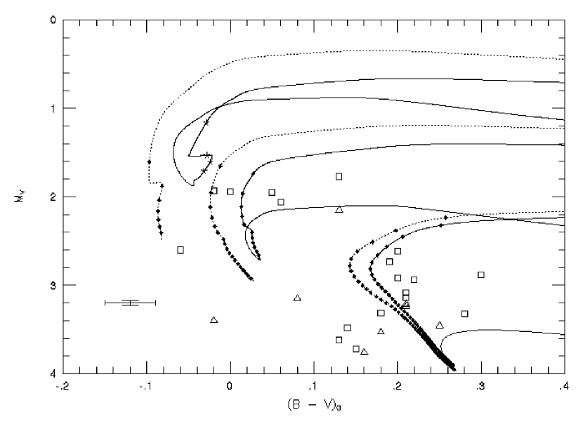
Figure 5: Color-magnitude diagram comparing our mixed and unmixed BSS models with observed BSSs in NGC 6397. The evolutionary tracks and filled symbols have the same meaning as in Figure 4. The blue straggler photometry is from Lauzeral et al. 1992 ($\Box$) and from Rubenstein & Bailyn 1996 ($\triangle$). The error bars indicate the maximum photometric errors for the BSSs quoted by Lauzeral et al. 1992.

4.2.1 Luminosity

A comparison of our evolutionary tracks with the photometry of BSSs in NGC 6397 is shown in Figure 5. Because of the overall helium enrichment in the remnants from prior evolution of the input stars, the luminosities of both the mixed and unmixed BSS models are higher than a zero-age star of the same mass. During the core hydrogen-burning phase, the luminosity of the unmixed model exceeds that of the mixed model, primarily because the early stages of core burning are avoided in the unmixed models. In any case, both sets of models can produce remnants of two-star collisions that have sufficient luminosity to explain the NGC 6397 observations.

The peak luminosities of our most massive BSS models ($\sim 2M_{TO}$) are larger than the brightest BSSs by nearly a magnitude. This could be explained if BSSs are not produced with this high a mass, or if the evolutionary timescales for high mass BSSs are very short compared to stragglers of lower mass. While we cannot directly test this first possibility, our BSS models show that our most massive unmixed model has a lifetime about 21% of the next most massive (a 12% decrease in mass). This may explain the lack of brighter blue stragglers.

If the no-mixing hypothesis is correct, then it may be necessary to invoke mass loss in excess of what is found in the hydrodynamical simulations. This could occur during spin-down of the merger remnant, possibly via a magnetic braking mechanism (Leonard & Livio 1995), even though our models never become fully convective. The energy input from the collision could cause the star to expand enough to have a significant convection zone (in mass and radius) without going deep enough to reach helium-enriched portions of the core. It is not currently known if BSSs in globular clusters are rotating rapidly or not, but BSSs in the open cluster M67 are known to have moderate rotation rates (between about 20 and 120 km/s; Peterson, Carney, & Latham 1984; Mathys 1991).

4.2.2 Absolute Colors

The evolutionary tracks for our most massive unmixed BSS models cover the colors of all but a few of the bluest stars. For the bright BSSs, the completely mixed models can cover even the bluest BSSs. However, for the faint BSSs though, neither set of models goes blue enough. Given that the total systematic uncertainties quoted by Lauzeral et al. (1993) are 0.1 mag in $(B-V)$, this color disagreement is not yet a serious problem. If the colors are accurately determined though, this must be explained.

Mass loss in addition to that resulting from the initial collision would further increase the disagreement. The metallicity we have used is probably at the low end of the acceptable range, so in all likelihood a change in the value of [Fe/H] for the cluster would also increase the disagreement. An abnormally low value of [$\alpha$/Fe] relative to other clusters could improve the color agreement, but this is unlikely.

The opacity data used in our models could also potentially affect the absolute colors. From comparisons that have been made between OPAL and Opacity Project datasets (Seaton et al. 1994), the opacities calculated using two different approaches agree to high accuracy. In addition, our comparisons of surface opacities (OPAL; Weiss et al. 1990; Alexander 1996) show that in the region of overlap that matters to our models, the agreement is also very good. For the surface temperatures of BSSs (relatively near the main sequence), uncertainties in surface opacities do not have an effect since molecular opacity, which is omitted in the OPAL calculations, does not become important until the star approaches the Hayashi track. We conclude that the opacities themselves are unlikely to explain the color mismatch.

4.2.3 Color Distribution

A quick examination of Figure 5 indicates that the models as they stand predict that BSSs should populate a smaller range of colors than is observed. In the past, this fact has not received much attention for several reasons. Photometric measurement and calibration errors both contribute to the scatter among the observed BSSs. In Figure 5, we have indicated the random errors in the BSS photometry of Lauzeral et al. (1992) to show that this source cannot explain the extra color scatter. In addition, observations have shown that there are other ways of producing objects that populate the regions where BSSs are found. Both detached and contact binaries are found among the BSS populations in NGC 4372 and NGC 5466. These examples show that stars that are in the process of merging can also be observed as blue stragglers. Our picture of merger remnants is undoubtedly confused by these stars in transit.

However, even among blue stragglers that are known to be single stars, the color scatter is real. SX Phe variables have been found in $\omega$ Cen (J$\o$rgensen 1982; J$\o$rgensen & Hansen 1984), NGC 5466 (Mateo et al. 1988), NGC 5053 (Nemec et al. 1995) and NGC 4372 (Kaluzny & Krzeminski 1993). The color distribution of samples of these stars provides a more definite indication of the color scatter, both because the pulsation mechanism can only operate in relatively relaxed single stars, and because these stars must be measured many times to derive light curves that show their identities.

In the globular cluster NGC 4372, 3 known SX Phe variables are significantly redder by about 0.2 in $(B-V)$ than the remaining 5, which may still form a fairly tight sequence (Kaluzny & Krzeminski 1993). One of the 5 known SX Phe variables in NGC 5466 (Nemec et al. 1995) is bluer than the others by about 0.15 in $(B-V$). The apparent bifurcation in color for these variables may be a result of different modes of pulsation. However, it does indicate significant color scatter among single stars.

Because stars evolve almost entirely to the red once core hydrogen has been exhausted, the apparent color width of the BSS sequence can indicate the amount of time a BSS spends completing core hydrogen burning compared to the time it spends as a subgiant. As can be seen from the evolutionary tracks shown in Figure 5, a completely-mixed remnant has a longer main-sequence lifetime, and spends a larger fraction of its remaining life close to a helium-enriched main sequence, prior to its turnoff from the main sequence. So, if massive BSSs were somehow completely mixed in all cases, they would define a comparatively thin extension of the cluster main sequence.

Our models, which show little mixing, are able to better explain the color width of the BSS sequence. If the high helium content of the core of a merger remnant is preserved, the main sequence phase is truncated, allowing the early subgiant branch phase of evolution to span a larger fraction of the remnant’s life. In addition, the pre-main-sequence-like phase of evolution follows the post-main-sequence evolution reasonably closely, slightly increasing the possibility that a remnant could be observed in the subgiant region of the CMD. But with the amount of mixing we find in our models, too much time is spent relatively close to the main sequence. This could be explained if the hydrodynamical mixing is overestimated in our simulations. This is possible, considering the arguments given in §3. It is also conceivable that one or both of the stars involved in a merger had evolved past the cluster turnoff, and hence has a higher core helium content to start. Due to their increased sizes, such stars have larger geometrical cross sections for collisions, and make binary mergers more likely due to increased tidal interactions.

As one looks fainter, the progenitor stars must become less massive. As a result, the cores of the remnant BSSs have lower helium contents. This means that unmixed models spend an increasing amount of time near the zero-age main sequence as the mass of the remnant decreases, which would lead to a definite concentration of stragglers toward the blue side of the region. As can be seen in Figure 4, the mixed and unmixed stars become more and more alike as BSS luminosity decreases. Unequal mass collisions would not help solve the problem — if the remnant is completely mixed, the lower mass star still contributes little helium, leading to a dilution; if unmixed, the lower entropy material of the low mass star would displace the relatively high entropy (and high helium content) matter at the core of the high mass star. In both cases, the core of the star still has a large amount of hydrogen, and will spend much of its life near the main sequence. An additional mechanism appears to be necessary to explain the color scatter at low BSS luminosity.

For the stars in NGC 6397 (and other clusters; Fusi Pecci et al. 1992), the scatter in the BSS colors appears to be inconsistent with both hypotheses as they stand, even if photometric scatter (0.03 mag in $V$ or $B-V$ at maximum; Lauzeral et al. 1992) is accounted for. Differential reddening is potentially more important for NGC 6397 because of its relatively large average reddening (E$(B-V)=0.18$; Peterson 1993). However, small color widths of the blue HB and of the RGB argue against this being a significant effect — variations of approximately 0.15 in E$(B-V)$ in the innermost $15^{\prime\prime}$ of the core would be necessary to make the brightest BSSs consistent with such a thin sequence. Further, the color scatter observed in the BSSs of many other clusters with much smaller reddenings cannot be explained this way.

For the distribution of blue stragglers to be explained by the evolution of stars more massive than the turnoff of the cluster, it seems that at least two things must occur. First, there must be a relatively large enrichment of helium in the envelope of the remnant star, which is required to explain the bluest of the stragglers. Second, there must also be nearly complete exhaustion of hydrogen in the core of the remnant, as required by the seemingly uniform color distribution of the stragglers in many clusters.

4.3 Advanced Evolutionary States

From our evolutionary tracks, we can predict regions in the color-magnitude diagram (CMD) where BSS progeny might be found. These topics have been discussed in other papers by Fusi Pecci et al. (1992) and Taam & Lin (1992). As red giants, evolved BSSs would be bluer than undisturbed cluster giants. As such, they would contribute to the color dispersion on the RGB (Taam & Lin 1992). Also, the most massive BSSs undergo helium flash at lower luminosities in our models than other stars. However, the RGB phase does not last long enough to be well-populated in cluster CMDs, and field stars also add to the confusion in the photometry, making it unlikely that evolved BSSs would be found on the RGB. Fusi Pecci et al. (1992) argue that clusters with the largest populations of BSSs will have an observable number of stars on the reddest end of the HB as a result of their higher mass relative to other cluster stars. Taam & Lin suggest that anomalous Cepheids may also be BSS progeny.

The mixing of helium into the stellar envelope will also affect the position of the HB stars in the CMD. In general, higher envelope helium abundance reduces the opacity, resulting in more compact, bluer stars. For massive HB stars though, increased helium abundance primarily increases the luminosity, but does not affect the color (Dorman 1992a). The complete mixing hypothesis would predict that the progeny of the most massive BSSs would have rather large envelope helium abundances, which would make them significantly more luminous than the rest of the HB, even to the point of looking like the faintest AGB stars.

More modest envelope enrichments occur in our unmixed models. The amount of enrichment is rather small (see §4.1.2), although slightly dependent on the energetics of the merger process, as higher energies imply slightly larger hydrodynamical mixing and, more importantly, deeper penetration of the convective envelope into helium-enriched regions during the pre-main-sequence-like phase.

From the models of Dorman (1992b), we can estimate the horizontal branch lifetime for massive BSS progeny. Assuming that there is mass loss between the RGB and HB of approximately $0.2M_{\odot}$ (which could produce the HB morphology of NGC 6397), an RGB mass of $1.5M_{\odot}$ could be reduced to $1.3M_{\odot}$. For an HB mass of $1.2M_{\odot}$, Dorman’s models predict that the core helium-burning lifetime is somewhat less than 90 Myr.

The two mixing hypotheses make different predictions for the relative number of BSSs and HB stars that are BSS progeny. Table 3 lists the ages of several points in the evolution of our BSS models — the start point, the first relaxed model (when the star begins a net absorption of thermal energy, as opposed to the thermal energy release during contraction), and the turnoff (bluest) model. The complete-mixing hypothesis predicts a BSS lifetime of approximately 0.65 Gyr for the most massive remnant. Our most massive model for the no-mixing hypothesis has a hydrogen burning lifetime of about 0.16 Gyr. Thus, unmixed models would predict approximately equal numbers of massive BSSs and their progeny, while completely-mixed models predict about 7 times as many massive BSSs as progeny.

The agreement of this ratio for completely-mixed models with the value of 6.6 from observations of globular clusters compiled by Fusi Pecci et al. (1992) should not be taken as evidence for that scenario, however. Because lower mass BSSs must also be present (inheriting lower core helium abundances, and thus longer lifetimes), unmixed models bracket the BSS lifetime predicted from HB models and observed BSS to BSS progeny ratios. Completely-mixed models have lifetimes that are in general too long.

5 Conclusions

1) From the results of our hydrodynamical simulations, we find that significant mixing from core to envelope does not occur in stellar interactions involving equal-mass stars, regardless of whether the interaction is a head-on or a grazing collision, or a binary merger. Grazing collisions and binary mergers result in slightly more mixing of helium into the envelope than do head-on collisions. (This result conflicts with the findings of Benz & Hills 1987.) Grazing collisions and binary mergers produce remnants that appear to be extremely similar.

Stars with lower central concentration (less dense cores) suffer slightly more hydrodynamical mixing, but not enough to alter the subsequent evolution of the remnant. Our analysis of the Goodman & Hernquist (1991) simulations of binary collisions indicate that these yield somewhat more hydrodynamical mixing than do single star collisions. As was found by Lombardi, Rasio, & Shapiro (1995) though, additional tests lead us to conclude that hydrodynamical mixing in our simulations is likely to be overestimated due to the finite spatial resolution of the gas in the model stars and the artificial diffusion that results.

2) Mass loss in our hydrodynamical simulations never exceeds 7% of the total mass of the merging stars, and so is insufficient to qualitatively alter our conclusions. Disks formed by stars colliding with the largest impact parameters can contain a significant amount of the total bound mass. In our analysis, we cannot estimate the amount of disk material that will be lost through angular momentum transfer during spin-down of the remnant. However, mass loss from a disk would only tend to increase the disagreement between our models and the observed colors of the hottest blue stragglers.

3) We have modeled the evolution of the merger remnants by imprinting helium profiles from hydrodynamical simulations onto one-dimensional stellar models. We have included effects of mass loss and energy input from the collision.

Typical energy inputs from the collisions are unable to provide the remnant with sufficient thermal energy to drive a convection zone large enough to mix core helium into the envelope. The energy input also temporarily quenches core convection in the more massive remnants by reducing the core temperature. The higher helium content of the core results in lower opacities, further preventing convective mixing of helium into the envelope even if the star does reach the Hayashi track. Additionally, thermally-relaxing remnants tend to reside in regions of the CMD populated by hydrostatic BSSs, making purely photometric separation impossible.

4) Unmixed models predict a lower limit for BSS lifetimes in NGC 6397 of about 0.1 Gyr for the most massive BSSs, while completely mixed models predict a minimum lifetime of about 0.6 Gyr.

For the most massive BSSs, completely mixed models can be as blue as the bluest BSSs, and the luminosity of the core hydrogen burning phase matches that of the brightest BSS in NGC 6397. However, these models cannot explain the reddest BSSs or the color scatter in the stragglers because they spend a large fraction of their time in the core hydrogen burning phase. The most massive unmixed models are more luminous than the brightest BSS during their main sequence phase, but also evolve rather quickly away from the main sequence which may make them less observable. Slightly lower mass models can reproduce the luminosity of the observed BSSs, but still have difficulty explaining the bluest BSSs, and the color scatter.

For faint BSS populations, the completely-mixed and unmixed evolutionary tracks have similar appearance because of the small amounts of core helium present in the progenitor stars. Both sets of models predict that the BSSs would inhabit a relatively large color range in the CMD, although with a concentration of stars on the blue side of the strip. Neither hypothesis is easily able to explain the bluest BSSs. This is in contradiction to the results of Proctor Sills, Bailyn, & Demarque (1995) because their study did not account for abundance enhancements in $\alpha$ elements that are known to occur in globular clusters.

The color width of the BSS sequences in many, if not all, globular clusters indicate that large portions of the lifetime of a blue straggler must be spent away from the zero-age main sequence. Completely mixed models cannot explain this observation because the star spends a large amount of time with comparatively high hydrogen content in the core, and hence lower luminosity and longer nuclear burning timescale. Unmixed models can potentially explain this observation because the vast majority of the core hydrogen-burning phase is avoided. Observations of SX Phe pulsating variables (which are presumably relatively relaxed single stars) in the clusters NGC 4372 and NGC 5466 indicate that there is significant color scatter among single star BSSs.

We must conclude that neither the completely mixed nor the unmixed hypothesis is able to consistently reproduce all details of the BSS distribution for NGC 6397, and that this would probably also apply to most other clusters. However, the main prediction of the complete mixing hypothesis — that blue stragglers produced by stellar collisions or binary mergers should populate a relatively thin locus in the CMD — appears to be untenable.

Table 1: Results of Main Sequence Stellar Evolution Calculations

$M/M_{\odot}$	Stage	Age (Gyr)	$E_{I}$	$E_{G}$	$\log R$ (cm)	$n_{eff}$
1.588	ZAMS	0.0	7.374	$-14.90$	10.844	3.06
	TO	1.1	7.377	$-14.85$	10.947	3.47
1.200	ZAMS	0.0	4.581	0$-9.25$	10.821	3.12
	TO	3.1	4.867	0$-9.79$	10.940	3.69
0.794	ZAMS	0.0	2.23	0$-4.50$	10.692	2.75
	TO	14.0	2.59	0$-5.20$	10.970	3.79
0.700	ZAMS	0.0	1.79	0$-3.62$	10.636	2.52
		14.0	1.91	0$-3.84$	10.702	2.99
0.596	ZAMS	0.0	1.37	0$-2.75$	10.563	2.18
0.401	ZAMS	0.0	0.73	0$-1.47$	10.412	1.61

Table 2: Results of SPH Calculations

Run	$M$	$\frac{(a+b)}{2c}$	$E_{K}$	$E_{I}$	$E_{G}$	$Y_{c}$
analytic polytrope models
$n=\frac{3}{2}$	1.000	1.000	0.000	0.429	$-0.857$
$n=3$	1.000	1.000	0.000	0.750	$-1.500$
$n=4$	1.000	1.000	0.000	1.500	$-3.000$
binary - binary collisions ($n=\frac{3}{2}$)
GH3	1.999	1.109	0.151	0.632	$-2.132$	0.78
GH6	2.928	1.049	0.130	0.630	$-3.213$	0.58
GH10	1.963	1.063	0.151	0.290	$-1.655$	0.79
GH22	3.812	1.017	0.139	0.892	$-4.329$	0.69
GH35	2.000	1.370	0.327	0.307	$-1.868$	0.79
GH43	2.940	1.301	0.409	0.446	$-2.768$	0.88
GH47	1.999	1.124	0.186	0.496	$-1.985$	0.74
GH49	2.945	1.204	0.335	0.624	$-3.283$	0.81
GH54	1.999	1.081	0.201	0.516	$-2.020$	0.70
GH57	1.971	1.142	0.201	0.412	$-1.846$	0.89
single star interactions ($n=\frac{3}{2}$)
HCQ1	1.948	1.019	0.003	0.505	$-1.922$	0.89
HCQ1BH	1.964	1.009	0.004	0.609	$-2.219$	0.96
GCQ1	1.986	1.104	0.159	0.162	$-1.421$	0.62
BMQ1	1.999	1.200	0.239	0.586	$-2.023$	0.94
single star interactions ($n=3$)
HCQ1	1.861	1.020	0.002	1.733	$-3.555$	0.83
HCQ1EM	1.855	1.007	0.004	1.894	$-3.814$	0.95
GCQ1	1.983	1.397	0.358	1.135	$-3.045$	0.85
BMQ1	1.996	1.297	0.354	1.388	$-3.557$	0.80

Table 3: Results of Blue Straggler Stellar Evolution Calculations

$M/M_{\odot}$	Stage	Age (yr)	$E_{I}$	$E_{G}$	$\log R$ (cm)	$n_{eff}$
unmixed models
1.478	ZA	0.0	0.61	0$-1.16$	11.719	2.15
	R	$2.2\times 10^{6}$	6.45	$-12.98$	11.007	3.69
	TO	$1.6\times 10^{8}$	6.45	$-12.97$	11.042	3.79
1.300	ZA	0.0	0.91	0$-1.83$	11.403	2.11
	R	$5.6\times 10^{6}$	5.45	$-10.98$	10.879	3.39
	TO	$7.8\times 10^{8}$	5.45	$-10.97$	10.957	3.66
1.071	ZA	0.0	0.59	0$-1.18$	11.358	1.63
	R	$1.4\times 10^{7}$	3.84	0$-7.75$	10.815	3.21
	TO	$3.65\times 10^{9}$	4.14	0$-8.32$	10.939	3.74
completely mixed models
1.478	ZA	0.0	6.97	$-14.06$	10.802	3.06
	TO	$6.5\times 10^{8}$	6.88	$-13.83$	10.918	3.49
1.300	ZA	0.0	5.44	$-10.99$	10.809	3.11
	TO	$1.57\times 10^{9}$	5.59	0$-11.25$	10.934	3.62
1.071	ZA	0.0	3.81	0$-7.70$	10.806	3.12
	TO	$4.07\times 10^{9}$	4.15	0$-8.34$	10.939	3.75

References

- (1)
- (2) Alexander, D. R. 1996, private communication
- (3)
- (4) Anthony-Twarog, B. J., Twarog, B. A., & Suntzeff, N. B. 1992, AJ, 103, 1264
- (5)
- (6) Aurière, M., Ortolani, S., & Lauzeral, C. 1990, Nature, 344, 638
- (7)
- (8) Bailyn, C. D. 1992, ApJ, 392, 519
- (9)
- (10) Bailyn, C. D. 1995, ARA&A, 33, 133
- (11)
- (12) Bailyn, C. D. & Pinsonneault, M. C. 1995, ApJ, 439, 705
- (13)
- (14) Benz, W. & Hills, J. G. 1987, ApJ, 323, 614
- (15)
- (16) Benz, W. & Hills, J. G. 1992, ApJ, 389, 546
- (17)
- (18) Carretta, E. & Gratton, R. G. 1996a, A&AS, in press
- (19)
- (20) Carretta, E. & Gratton, R. G. 1996b, in ASP Conf. Ser. 92, Formation of the Galactic Halo…Inside and Out, ed. H. Morrison and A. Sarajedini, (San Francisco: ASP), 363
- (21)
- (22) Chieffi, A., Straniero, O., & Salaris, M. 1991, in ASP Conf. Ser. 13, The Formation and Evolution of Star Clusters, ed. K. Janes (San Francisco: ASP), 219
- (23)
- (24) Dorman, B. 1992a, ApJS, 80, 701
- (25)
- (26) Dorman, B. 1992b, ApJS, 81, 221
- (27)
- (28) Eggleton, P. P. 1991, private communication
- (29)
- (30) Eggleton, P. P., Faulkner, J., & Flannery, B. P. 1973, A&A, 23, 325
- (31)
- (32) Ferraro, F. R., Fusi Pecci, F., Cacciari, C., Corsi, C., Buonanno, R., Fahlman, G. G., & Richer, H. B. 1993, AJ, 106, 2324
- (33)
- (34) Fusi Pecci, F., Ferraro, F. R., Corsi, C. E., Cacciari, C., & Buonanno, R. 1992, AJ, 104, 1831
- (35)
- (36) Goodman, J. & Hernquist, L. 1991, ApJ, 378, 637
- (37)
- (38) Gratton, R. G., Quarta, M. & Ortolani, S. 1986, A&A, 169, 208
- (39)
- (40) Hernquist, L. 1993, ApJ, 404, 717
- (41)
- (42) Hernquist, L. & Katz, N. 1989, ApJS, 70, 419
- (43)
- (44) Hodder, P. J. C., Nemec, J. M., Richer, H. B., & Fahlman, G. G. 1992, AJ, 103, 460
- (45)
- (46) Hut, P., et al. 1992, PASP, 104, 981
- (47)
- (48) Iglesias, C. A., Rogers, F. J. & Wilson, B. G. 1992, ApJ, 397, 717
- (49)
- (50) Jrgensen, H. E. 1982, A&A, 108, 99
- (51)
- (52) Jrgensen, H. E. & Hansen, L. 1984, A&A, 133, 165
- (53)
- (54) Kaluzny, J. & Krzeminski, W. 1993, MNRAS, 264, 785
- (55)
- (56) Lai, D., Rasio, F. A., & Shapiro, S. L. 1993, ApJ, 412, 593
- (57)
- (58) Lambert, D. L., McWilliam, A., & Smith, V. V. 1992, ApJ, 386, 685
- (59)
- (60) Lauzeral, C., Aurière, M., & Coupinot, G. 1993, A&A, 274, 214
- (61)
- (62) Lauzeral, C., Ortolani, S., Aurière, M., & Melnick, J. 1992, A&A, 262, 63
- (63)
- (64) Lee, Y.-W., Demarque, P., & Zinn, R. 1990, ApJ, 350, 155
- (65)
- (66) Leonard, P. J. T. & Livio, M. 1995, ApJ, 447, L121
- (67)
- (68) Lombardi, J. C., Rasio, F. A., & Shapiro, S. L. 1995, ApJ, 445, L117
- (69)
- (70) Mateo, M., Harris, H. C., Nemec, J., Olszewski, E., & Schombert, J. 1988, BAAS, 20, 717
- (71)
- (72) Mateo, M., Harris, H. C., Nemec, J., & Olszewski, E. W. 1990, AJ, 100,469
- (73)
- (74) Mathys, G. 1991, A&A, 245, 467
- (75)
- (76) Monaghan, J. J. 1992, ARA&A, 30, 543
- (77)
- (78) Monaghan, J. J. & Lattanzio, J. C. 1985, A&A, 149, 135
- (79)
- (80) Nemec, J. M. & Cohen, J. G. 1989, ApJ, 336, 780
- (81)
- (82) Nemec, J. M., Mateo, M., Burke, M., & Olszewski, E. W. 1995, AJ, 110, 1186
- (83)
- (84) Niss, B., Jrgensen, H. E., & Lausten, S. 1978, A&AS, 32, 387
- (85)
- (86) Paresce, F., et al. 1991, Nature, 352, 297
- (87)
- (88) Peterson, C. J. 1993, in ASP Conf. Ser. 50, Structure and Dynamics of Globular Clusters, ed. S. G. Djorgovski and G. Meylan (San Francisco: ASP), 337
- (89)
- (90) Peterson, R. C., Carney, B. W., & Latham, D. W. 1984, ApJ, 279, 237
- (91)
- (92) Pilachowski, C. A. 1984, ApJ, 281, 614
- (93)
- (94) Pilachowski, C. A., Olszewski, E. W. & Odell, A. 1983, PASP, 95, 713
- (95)
- (96) Proctor Sills, A., Bailyn, C. D., & Demarque, P. 1995, ApJ, 455, L163
- (97)
- (98) Rasio, F. A. & Shapiro, S. L. 1995, 438, 887
- (99)
- (100) Rogers, F. J., 1996, private communication
- (101)
- (102) Rubenstein, E. P. & Bailyn, C. D. 1996, AJ, 111, 260
- (103)
- (104) Seaton, M. J., Yan, Y., Mihalas, D., & Pradhan, A. K. 1994, MNRAS, 266, 805
- (105)
- (106) Smith, H. A. 1984, ApJ, 281, 148
- (107)
- (108) Stryker, L. L. 1993, PASP, 105, 1081
- (109)
- (110) Taam, R. E. & Lin, D. N. C. 1992, ApJ, 390, 440
- (111)
- (112) VandenBerg, D. A. 1992, ApJ, 391, 685
- (113)
- (114) Weiss, A., Keady, J. J., & Magee, N. H. 1990, Atomic Data and Nuclear Data Tables, 45, 209
- (115)
- (116) Yan, L. & Mateo, M. 1994, AJ, 108, 1810
- (117)
- (118) Yan, L. & Reid, I. N. 1996, MNRAS, 279, 751
- (119)
- (120) Yanny, B., Guhathakurta, P., Bahcall, J. N., & Schneider, D. P. 1994a, AJ, 107, 1745
- (121)
- (122) Yanny, B., Guhathakurta, P., Schneider, D. P, & Bahcall, J. N. 1994b, ApJ, 435, 59
- (123)
- (124) Zinn, R. & West, M. J. 1984, ApJS, 55, 45
- (125)