Molecular Hydrogen in the Direction of $\zeta$ Ori A

Abstract

A spectrum of $\zeta$ Ori A over the wavelength interval 950$-$1150Å recorded by Interstellar Medium Absorption Profile Spectrograph (IMAPS) on the ORFEUS-SPAS I mission shows Lyman and Werner band absorption features from molecular hydrogen in rotational levels $J=0$, 1, 2, 3 and 5. Most of the molecules are found in two distinct velocity components. One is at a heliocentric radial velocity of about $-$1 km s^-1 with $\log N({\rm H}_{2})=14.5$ and a rotational temperature $T_{\rm rot}=950$K, while the other is at +25 km s^-1 with $\log N({\rm H}_{2})=15.9$ and $T_{\rm rot}=320$K. Some extra H₂ exists in a much weaker component ($\log N({\rm H}_{2})=14.0$) between the two main peaks.

The H₂ component at $-$1 km s^-1 exhibits profile shapes that become broader and show small displacements toward more negative velocities as $J$ increases. These changes are inconsistent with a simple interpretation that uv optical pumping in an optically thin, uniform medium creates the H₂ in excited rotational levels. Differential shielding of the uv radiation at certain velocities does not appear to be a satisfactory explanation for the effect.

Evidence from atomic features at other velocities may offer some insight on the origin of this unusual behavior exhibited by the H₂ profiles. Absorption features from moderately ionized atoms at $-$94 km s^-1 and more highly ionized species at about $-$36 km s^-1 suggest that along the line of sight to $\zeta$ Ori A there may be a standing bow shock with an initial compression ratio of 2.6. This shock is probably created when a negative-velocity gas flow collides with an obstruction, in this case a neutral cloud at 0 km s^-1. If this interpretation is correct, the H₂ with the changing profiles may represent molecules forming in the postshock gas flow that is undergoing further compression as it recombines and cools. We suggest that molecules can form initially by associative detachment of H^- in a moving, warm, partly ionized medium behind the front. The H₂ in this area is most conspicuous in the higher $J$ levels. Later, when the gas becomes very cool, neutral, and more compressed as it comes nearly to a halt, it is more easily seen in the lowest $J$ levels. In this part of the medium, the principal way of producing H₂ should be from reactions on the surfaces of dust grains, as one expects for quiescent interstellar clouds.

1 Introduction

The first detection of hydrogen molecules in space came from a distinctive pattern of absorption features that appeared in a low resolution uv spectrum of $\xi$ Per recorded by a spectrometer on a sounding rocket (Carruthers 1970). Starting with that pioneering discovery, the Lyman and Werner bands of H₂ in the spectra of early-type stars have led us down a trail of new discoveries about this most abundant molecule in space. Progressively more refined observations by the Copernicus satellite have given us a fundamental understanding on this molecule’s abundances in various diffuse cloud environments (Spitzer et al. 1973; York 1976; Savage et al. 1977), how rapidly it is created and destroyed in space (Jura 1974), and the amount of rotational excitation that is found in different circumstances (Spitzer & Cochran 1973; Spitzer, Cochran, & Hirshfeld 1974; Morton & Dinerstein 1976). The observed populations in excited rotational levels have in turn led to theoretical interpretations about how this excitation is influenced by such conditions as the local gas density, temperature and the flux of uv pumping radiation from nearby stars (Spitzer & Zweibel 1974; Jura 1975a, b). Many of the highlights of these investigations have been reviewed by Spitzer & Jenkins (1975) and Shull & Beckwith (1982). The Lyman and Werner bands of H₂ can even be used to learn more about the properties of very distant gas systems whose absorption lines appear in quasar spectra (Foltz, Chaffee, & Black 1988; Songaila & Cowie 1995), although the frequency of finding these H₂ features is generally quite low (Levshakov et al. 1992).

In addition to the general conclusions just mentioned, there were some intriguing details that came from the observations of uv absorption lines. The early surveys by the Copernicus satellite indicated that toward a number of stars the H₂ features became broader as the rotational quantum number $J$ increased (Spitzer & Cochran 1973; Spitzer, Cochran, & Hirshfeld 1974). An initial suggestion by Spitzer & Cochran (1973) was that the extra broadening of the higher $J$ levels could arise from new molecules that had a large kinetic energy that was liberated as they formed and left the grain surfaces. However, a more detailed investigation by Spitzer & Morton (1976) showed that, as a rule, the cases that exhibited the line broadening with increasing $J$ were actually composed of two components that had different rotational excitations and a velocity separation that was marginally resolved by the instrument. In general, they found that the component with a more negative radial velocity was relatively inconspicuous at low $J$, but due to its higher rotation temperature it became more important at higher $J$ and made the composite profile look broader.

By interpreting the rotational populations from the standpoint of theories on collisional and uv pumping, Spitzer & Morton (1976) found a consistent pattern where the components with the most negative velocity in each case had extraordinarily large local densities and exposure to unusually high uv pumping fluxes. They proposed that these components arose from thin, dense sheets of H₂-bearing material in the cold, compressed regions that followed shock fronts coming toward us. These fronts supposedly came from either the supersonic expansions of the stars’ H II regions or perhaps from the blast waves caused by supernova explosions in the stellar associations.

Now, some twenty years after the original investigations with the Copernicus satellite, we have an opportunity to study once again the behavior of the H₂ profiles, but this time with a wavelength resolution that can cleanly separate the components. We report here the results of an investigation of H₂ toward $\zeta$ Ori A, one of the stars studied earlier that showed the intriguing behavior with the H₂ components discussed above. Once again, the concept of the H₂ residing in the dense gas behind a shock comes out as a central theme in the interpretation, but our description of the configuration given in §5.2 is very different from that offered by Spitzer & Morton (1976).

2 Observations

The Lyman and Werner band absorptions of H₂ in the spectrum of $\zeta$ Ori A were observed with the Interstellar Medium Absorption Profile Spectrograph (IMAPS). IMAPS is an objective-grating echelle spectrograph that was developed in the 1980’s as a sounding rocket instrument (Jenkins et al. 1988, 1989) and was recently reconfigured to fly in orbit. It can record the spectrum of a star over the wavelength region 950$-$1150Å at a resolving power of about 200,000. This instrument flew on the ORFEUS-SPAS carrier launched on 12 September 1993 by the Space Shuttle flight STS-51. Jenkins, et al. (1996) have presented a detailed description of IMAPS, how it performed during this mission and how the data were reduced. Their article is especially useful for pointing out special problems with the data that were mostly overcome in the reduction. It also shows an image of a portion of the echelle spectrum of $\zeta$ Ori A.

The total exposure time on $\zeta$ Ori was 2412 s, divided among 63 frames, each of which covered ¼ of the echelle’s free spectral range. Spectra were extracted using an optimal extraction routine described by Jenkins, et al. (1996), and different measurements of the intensity at any given wavelength were combined with weights proportional to their respective inverse squares of the errors. Samples of some very restricted parts of the final spectrum are shown in Fig. 1, where lines from $J$ = 0, 1, 3 and 5 may be seen.

Figure 1: Sample wavelength intervals covering four H₂ lines in the spectrum of $\zeta$ Ori recorded by IMAPS. The intensity scale is in photons per detector pixel. Except for the transition out of $J=5$, two prominent velocity components are seen in each H₂ line, one at a heliocentric radial velocity of about $-$1 km s^-1 (labeled with marks that identify the transitions) and another at +25 km s^-1. Detector pixels are oversampled by a factor of two in this figure. Dashed lines show the amplitude of ten times the expected standard deviation of the points resulting from photon counting statistics.

3 Data Reduction

3.1 Wavelength Scale and Resolution

Since IMAPS is an objective-grating instrument, there is no way that we can use an internal line emission light source to provide a calibration of the wavelength scale. However, as explained in Jenkins, et al. (1996), we have an accurate knowledge of how the apparent detector coordinates map into real geometrical coordinates on the image plane, and we also know the focal length of the cross-disperser grating and the angles of incidence and diffraction for the echelle grating. The only unknown parameter that we must measure is a zero offset that is driven by the pointing of IMAPS relative to the target. We determined this offset by measuring the positions of telluric absorption features of O I in excited fine-structure levels. These features are rarely seen in the interstellar medium, but there is enough atmospheric oxygen above the orbital altitude of 295 km to produce the absorption features in all of our spectra.

To obtain a wavelength scale that would give heliocentric velocities for all of our lines, we adjusted the zero offset so that the telluric features appeared at +27.0 km s^-1, a value that was appropriate for the viewing direction and time of our observations. The general accuracy of our wavelength scale is indicated by the fact that oxygen lines in 4 different multiplets all gave velocities within 0.5 km s^-1 of the average. Also, for H₂ lines out of a given $J$ level that had roughly comparable transition strengths, the dispersion of measured velocities was about 0.5 km s^-1. The measured position of the strongest component (for all $J$ levels) of 24.5 km s^-1 compares favorably with the heliocentric velocity of a strong, but complex absorption feature of Na I centered on 24 km s^-1 (Welty, Hobbs, & Kulkarni 1994).

The excited O I lines can also be used to give an indication of the wavelength resolution of our observations. We measured equivalent widths of 10.5 and 7.25mÅ for the O I^∗ and O I^∗∗ lines at 1040.9 and 1041.7Å, respectively. For the applicable densities and temperatures of the Earth’s upper atmosphere, the occupation of the singly excited level (O I^∗) should be 3 times that of the doubly excited level (O I^∗∗), i.e., their relative numbers are governed by just their statistical weights $g$. Making use of this fact allows us to apply a standard curve of growth analysis to derive log N(O I^∗∗) = 14.19 and $b=0.99~{}{\rm km~{}s}^{-1}$ (equivalent to a doppler broadening for $T=950$K). The observed profiles have widths that correspond to $b=3.0~{}{\rm km~{}s}^{-1}$, which leads to the conclusion that the instrumental spread function is equivalent to a profile with

$$b_{\rm inst}=\sqrt{3.0^{2}-1.25^{2}}=2.7~{}{\rm km~{}s}^{-1}$$ (1)

(The representative $b$ for the excited O I lines has been elevated to 1.25 km s^-1 to account for the small broadening caused by saturation).

The wavelength resolving power that we obtained is lower than what is achievable in principle with IMAPS and the pointing stability of the spacecraft. We attribute the degradation to small motions of the echelle grating during the exposures, caused by a sticky bearing that relieved mechanical stresses at random times. The magnitude and character of this effect is discussed in detail by Jenkins, et al. (1996).

3.2 Absorption Line Measurements

We used the MSLAP analysis program to define the continuum level $I_{0}$ and re-express the intensities $I(v)$ in terms of the apparent absorption optical depths $\tau_{a}$ as a function of radial velocity,

$$\tau_{a}(v)=\ln\Bigl{(}{I_{0}\over I(v)}\Bigr{)}~{}.$$ (2)

For the ideal case where the instrument can resolve the finest details in velocity, $\tau_{a}(v)$ usually gives an accurate depiction of a differential column density per unit velocity through the relation

$$N_{a}(v)=3.768\times 10^{14}{\tau_{a}(v)\over f\lambda}{\rm cm}^{-2}({\rm km~{}s}^{-1})^{-1}~{},$$ (3)

where $f$ is the transition’s $f$-value and $\lambda$ is expressed in Å. However, if there are saturated, fine-scale details that are not resolved, the true optical depths $\tau(v)$ averaged over velocity will be underestimated, and one will miscalculate the true column density $N(v)$. One can ascertain that this is happening if the application of Eq. 3 for weaker lines indicates the presence of more material than from the strong ones (Savage & Sembach 1991; Jenkins 1996). As will be evident in §4.1, this appears to happen for the strongest features of H₂ in the $J$ = 0, 1 and 2 levels of rotational excitation.

For $J$ levels 0 through 3, we were able to draw together the results for many different absorption lines, each going to different rotational and vibrational levels in the upper electronic states, 2p$\sigma\,B\,^{1}\Sigma_{u}^{+}$ and 2p$\pi\,C\,^{1}\Pi_{u}$. In so doing, it was important to keep track of the errors in the measured $I(v)$ and combine redundant information at each velocity in a manner that lowered the error in the final result. To achieve this goal, we evaluated for every individual velocity point the $\chi^{2}$ from a summation over the separate transitions,

$$\chi^{2}(\tau_{a})=\sum\biggl{(}{\exp(-\tau_{a})-I/I_{0}\over\epsilon(I/I_{0})}\biggr{)}^{2}~{}.$$ (4)

The expected errors in intensity $\epsilon(I/I_{0})$ represented a combination of several sources of error: (1) the noise in the individual measurements of $I$, (2) an error in the placement of the continuum $I_{0}$, and (3) an error in the adopted value of zero spectral intensity (which is a finite value of real intensity extracted from the echelle order). The errors in $I$ (item 1) were measured from the dispersion of residual intensities on either side of the adopted continuum at points well removed in velocity from the absorption feature. This error generally becomes larger at progressively shorter wavelengths, because the sensitivity of IMAPS decreases. (Variations of sensitivity also result from being away from the center of the echelle blaze function.) In every case, the noise errors were assumed to be the same magnitude at low $I/I_{0}$ at the centers of lines because statistical fluctuations in the background illumination are important. (Generally, the background was about as large as $I_{0}$, so the noise amplitude would decrease only by a factor of $\sqrt{2}$.) In a number of cases, the computed S/N was higher than 50 (see Tables 1$-$4). Because there might be some residual systematic errors that we have not recognized, we felt that it was unwarranted to assume that these cases had the full reliability as indicated by the calculation of S/N, when compared with other measurements at lower S/N. To account for this, we uniformly adopted an estimate for the relative noise level consistent with the value

$${\rm adopted~{}S/N}=1/\sqrt{({\rm computed~{}S/N})^{-2}+50^{-2}}.$$ (5)

The error in $I_{0}$ (item 2 in the above paragraph) represents the uncertainty of the continuum level that arises from a pure vertical translation that would be permitted by the noise in the many intensity measurements that define $I_{0}$. It does not include errors in the adopted curvature of the continuum [see a discussion of this issue in the appendix of Sembach & Savage (1992)]. For most cases, the curvature was almost nonexistent. The error in the adopted background level (item 3) was judged from the dispersion of residual intensities of saturated atomic lines elsewhere in the spectrum. At every velocity point, the worst combinations of the systematic errors (i.e., both the adopted continuum and background levels are simultaneously too high or, alternatively, too low) were combined in quadrature with the random intensity errors (item 1), as modified in Eq. 5, to arrive at the net $\epsilon(I/I_{0})$.

Tables 1$-$4 show the transitions for the four lowest rotational levels of H₂ covered in our spectrum of $\zeta$ Ori. Laboratory wavelengths are taken from the calculated values of Abgrall, et al. (1993a) for the Lyman band system and Abgrall, et al. (1993b) for the Werner bands. Transition $f$-values are from Abgrall & Roueff (1989). The listed values of S/N are those computed as described above, but without the modification from Eq. 5.

All of the lines for $J$ = 4 were too weak to measure. Only one line from $J$ = 5 was strong enough to be useful (the Werner 0$-$0 Q(5) line at 1017.831Å with $\log(f\lambda)$ = 1.39), although weaker lines showed very noisy profiles that were consistent with this line.

Many lines (or certain portions thereof) were unsuitable for measurement. These lines and the reasons for their rejection are discussed in the endnotes of the tables. Table 4 omits some lines that are far too weak to consider.

Table 1: Lines from J=0

Ident.	$\lambda$ (Å)	Log ($f\lambda$)	S/N
0$-$0 R(0)	1108.127	0.275	50
1$-$0 R(0)string	1092.195	0.802	77
2$-$0 R(0)string	1077.140	1.111	46
3$-$0 R(0)string	1062.882	1.282	45
4$-$0 R(0)string	1049.367	1.383	30
5$-$0 R(0)string	1036.545	1.447	39
6$-$0 R(0)string	1024.372	1.473	36
7$-$0 R(0)string	1012.810	1.483	81
8$-$0 R(0)string	1001.821	1.432	32
9$-$0 R(0)	991.376	1.411	$\cdots$
10$-$0 R(0)	981.437	1.314	23
11$-$0 R(0)	971.985	1.289	$\cdots$
12$-$0 R(0)	962.977	1.098	14
13$-$0 R(0)	954.412	1.126	20
W 0$-$0 R(0)	1008.552	1.647	31
W 1$-$0 R(0)	985.631	1.833	$\cdots$
W 2$-$0 R(0)	964.981	1.823	$\cdots$

Table 2: Lines from J=1

Ident.	$\lambda$ (Å)	Log ($f\lambda$)	S/N
0$-$0 P(1)	1110.062	$-$0.191	46
1$-$0 P(1)	1094.052	0.340	40
2$-$0 P(1)string	1078.927	0.624	33
3$-$0 P(1)string	1064.606	0.805	48
4$-$0 P(1)string	1051.033	0.902	48
5$-$0 P(1)string	1038.157	0.956	78
6$-$0 P(1)	1025.934	0.970	$\cdots$
7$-$0 P(1)string	1014.325	0.960	62
8$-$0 P(1)string	1003.294	0.931	19
9$-$0 P(1)	992.808	0.883	14
10$-$0 P(1)	982.834	0.825	14
11$-$0 P(1)	973.344	0.759	3
12$-$0 P(1)	964.310	0.683	12
13$-$0 P(1)	955.707	0.604	9
W 0$-$0 Q(1)string	1009.770	1.384	36
W 1$-$0 Q(1)	986.796	1.551	8
W 2$-$0 Q(1)	966.093	1.529	10
0$-$0 R(1)	1108.632	0.086	39
1$-$0 R(1)	1092.732	0.618	69
2$-$0 R(1)string	1077.700	0.919	55
3$-$0 R(1)string	1063.460	1.106	59
4$-$0 R(1)string	1049.960	1.225	64
5$-$0 R(1)string	1037.149	1.271	56
6$-$0 R(1)	1024.986	1.312	11
7$-$0 R(1)string	1013.434	1.307	48
8$-$0 R(1)string	1002.449	1.256	16
9$-$0 R(1)	992.013	1.252	19
10$-$0 R(1)	982.072	1.138	14
11$-$0 R(1)	972.631	1.134	5
12$-$0 R(1)	963.606	0.829	12
13$-$0 R(1)	955.064	0.971	9W 0$-$0 R(1)	1008.498	1.326	$\cdots$
W 1$-$0 R(1)	985.642	1.512	$\cdots$
W 2$-$0 R(1)	965.061	1.529	$\cdots$

Table 3: Lines from J=2

Ident.	$\lambda$ (Å)	Log ($f\lambda$)	S/N
0$-$0 P(2)	1112.495	$-$0.109	39
1$-$0 P(2)	1096.438	0.420	51
2$-$0 P(2)string	1081.266	0.706	55
3$-$0 P(2)	1066.900	0.879	65
4$-$0 P(2)string	1053.284	0.982	35
5$-$0 P(2)string	1040.366	1.017	38
6$-$0 P(2)	1028.104	1.053	13
7$-$0 P(2)	1016.458	1.007	34
8$-$0 P(2)string	1005.390	0.998	29
9$-$0 P(2)	944.871	0.937	18
10$-$0 P(2)	984.862	0.907	5
11$-$0 P(2)	975.344	0.809	7
12$-$0 P(2)	966.273	0.798	13
13$-$0 P(2)	957.650	0.662	12
W 0$-$0 P(2)	1012.169	0.746	23
W 1$-$0 P(2)	989.086	0.904	8
W 2$-$0 P(2)	968.292	0.843	14
W 0$-$0 Q(2)string	1010.938	1.385	29
W 1$-$0 Q(2)	987.972	1.551	7
W 2$-$0 Q(2)	967.279	1.530	11
0$-$0 R(2)	1110.119	0.018	45
1$-$0 R(2)	1094.243	0.558	56
2$-$0 R(2)	1079.226	0.866	35
3$-$0 R(2)string	1064.994	1.069	53
4$-$0 R(2)string	1051.498	1.168	76
5$-$0 R(2)string	1038.689	1.221	72
6$-$0 R(2)	1026.526	1.267	$\cdots$
7$-$0 R(2)string	1014.974	1.285	52
8$-$0 R(2)string	1003.982	1.232	40
9$-$0 R(2)string	993.547	1.228	20
10$-$0 R(2)string	983.589	1.072	18
11$-$0 R(2)	974.156	1.103	4
12$-$0 R(2)	965.044	0.161	$\cdots$
13$-$0 R(2)	956.577	0.940	10
W 0$-$0 R(2)string	1009.024	1.208	32
W 1$-$0 R(2)	986.241	1.409	3W 2$-$0 R(2)string	965.791	1.490	16

Table 4: Lines from J=3

Ident.	$\lambda$ (Å)	Log ($f\lambda$)	S/N
0$-$0 P(3)	1115.895	$-$0.083	45
1$-$0 P(3)	1099.787	0.439	31
2$-$0 P(3)	1084.561	0.734	$\cdots$
3$-$0 P(3)string	1070.141	0.910	26
4$-$0 P(3)string	1056.472	1.006	56
5$-$0 P(3)string	1043.502	1.060	48
6$-$0 P(3)string	1031.192	1.055	41
7$-$0 P(3)string	1019.500	1.050	57
8$-$0 P(3)	1008.383	1.004	$\cdots$
9$-$0 P(3)	997.824	0.944	18
10$-$0 P(3)	987.768	0.944	10
11$-$0 P(3)	978.217	0.817	20
12$-$0 P(3)	969.089	0.895	10
13$-$0 P(3)	960.449	0.673	12
W 0$-$0 P(3)string	1014.504	0.920	54
W 1$-$0 P(3)	991.378	1.075	$\cdots$
W 2$-$0 P(3)	970.560	0.974	10
W 0$-$0 Q(3)string	1012.680	1.386	31
W 1$-$0 Q(3)	989.728	1.564	$\cdots$
W 2$-$0 Q(3)	969.047	1.530	8
0$-$0 R(3)	1112.582	$-$0.024	$\cdots$
1$-$0 R(3)	1096.725	0.531	$\cdots$
2$-$0 R(3)string	1081.712	0.840	47
3$-$0 R(3)string	1067.479	1.028	42
4$-$0 R(3)string	1053.976	1.137	37
5$-$0 R(3)string	1041.157	1.222	49
6$-$0 R(3)string	1028.985	1.243	24
7$-$0 R(3)string	1017.422	1.263	35
8$-$0 R(3)string	1006.411	1.207	18
9$-$0 R(3)string	995.970	1.229	33
10$-$0 R(3)	985.962	0.908	4
11$-$0 R(3)	976.551	1.104	$\cdots$
12$-$0 R(3)	967.673	1.347	10
13$-$0 R(3)	958.945	0.931	10
W 0$-$0 R(3)	1010.129	1.151	40
W 1$-$0 R(3)	987.445	1.409	6W 2$-$0 R(3)	966.780	0.883	16

4 Results

Figs. 2$-$6 show gray-scale representations of $\chi^{2}-\chi_{\rm min}^{2}$ as a function of $\log N_{a}(v)$ and the heliocentric radial velocity $v$. The minimum value $\chi_{\rm min}^{2}$ was determined at each velocity, and our representation that shows how rapidly $\chi^{2}$ increases on either side of the most probable $\log N_{a}(v)$ (i.e., the value where $\chi_{\rm min}^{2}$ is achieved) is a valid measure of the relative confidence of the result (Lampton, Margon, & Bowyer 1976). Since we are measuring a single parameter, the $\chi^{2}$ distribution function with 1 degree of freedom is appropriate, and thus, for example, 95% of the time we expect the true intensity to fall within a band where $\chi^{2}-\chi_{\rm min}^{2}<3.8$, i.e., the “$\pm 2\sigma$” zone. To improve on the range of the display without sacrificing detail for low values of $\chi^{2}-\chi_{\rm min}^{2}$, the actual darknesses in the figures and their matching calibration squares on the right are scaled to the quantity $\log(1+\chi^{2}-\chi_{\rm min}^{2})$. Measurements at velocities separated by more than a single detector pixel (equivalent to 1.25 km s^-1) should be statistically independent. This separation is less than the wavelength resolving power however. Thus, reasonable assumptions about the required continuity of the profiles for adjacent velocities can, in principle, restrict the range of allowable departures from the minimum $\chi^{2}$ even further than the formal confidence limits.

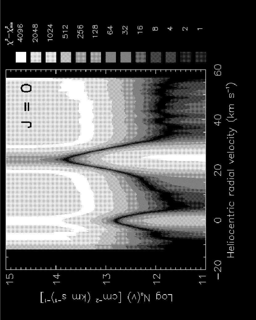
Figure 2: A composite of 8 absorption profiles from H₂ in the $J$ = 0 rotational level. Transitions listed in Table 1 were used, except where noted. Shades of gray, as indicated by the boxes on the right, map out the changes in $\chi^{2}-\chi_{\rm min}^{2}$ as a function of $\log N_{a}(v)$ for each value of $v$. For reasons discussed in §4.1 the strong peak on the right-hand side probably understates the true amount of H₂ that is really present.

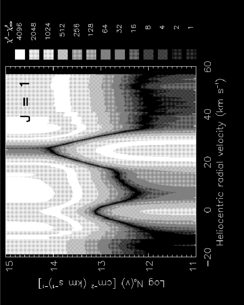
Figure 3: Same as for Fig. 2, except that the applicable transitions, listed in Table 2, are from the $J$ = 1 level. Thirteen transitions were combined to make this figure. As with Fig. 2, the rightmost, strong peak probably under-represents the true amount of H₂.

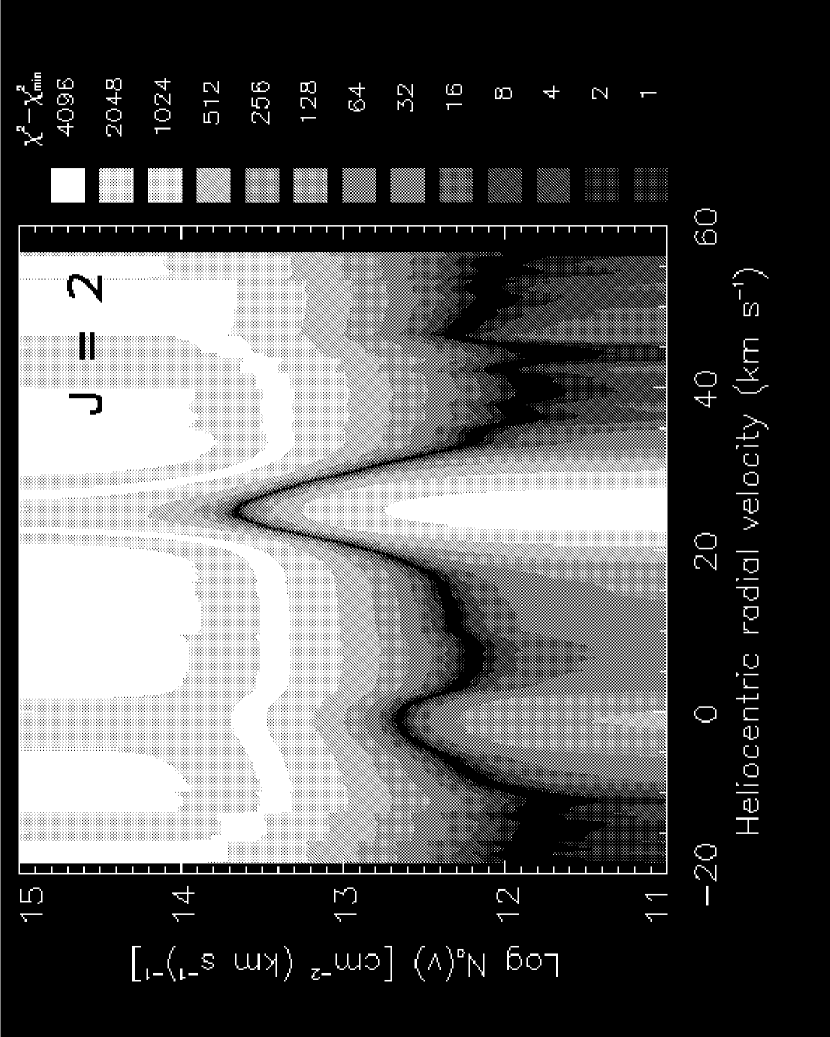
Figure 4: Same as for Fig. 2, except that the applicable transitions, listed in Table 3, are from the $J$ = 2 level. A total of 19 transitions were used to construct this figure, but because of interference problems only 14 of them covered Components 1 and 2.

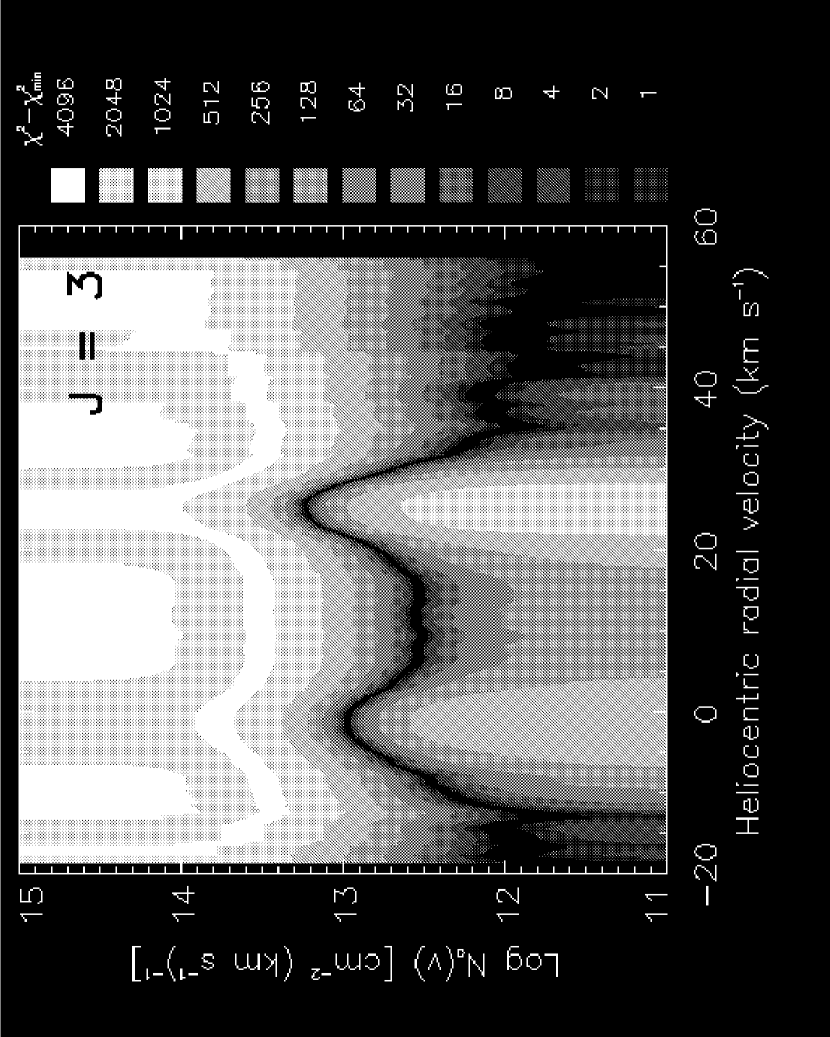
Figure 5: Same as for Fig. 2, except that the 15 applicable transitions, listed in Table 4, are from the $J$ = 3 level. Unlike the cases for $J$ = 0, 1 or 2, the right-hand peak does not show any disparities in the height from one transition to another, indicating that the representation is probably correct.

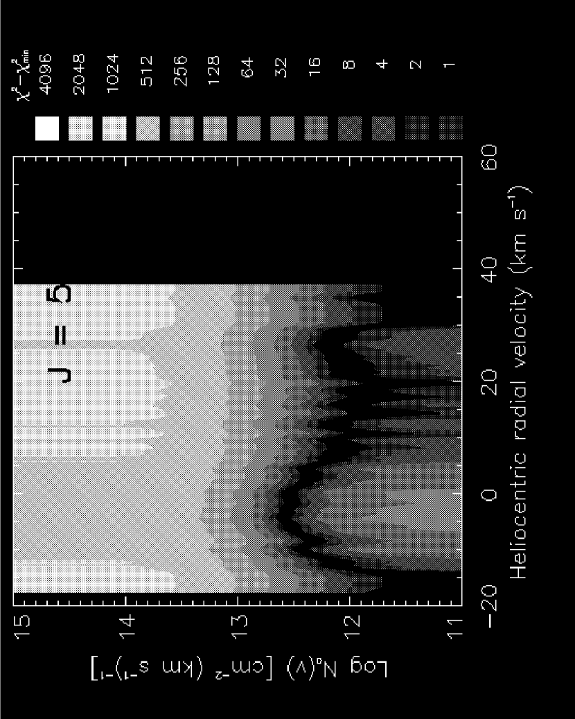
Figure 6: Same as for Fig. 2, except that only one transition, the Werner 0$-$0 Q(5) line, was used.

The profiles that appear in Figs. 2$-$6 indicate that there are two prominent peaks in H₂ absorption, with the left-hand one holding molecules with a higher rotational temperature than the one on the right. This effect, one that creates dramatic differences in the relative sizes of the two peaks with changing $J$, was noted earlier by Spitzer, et al. (1974). There is also some H₂ that spans the velocities between these two peaks. For the purposes of making some general statements about the H₂, we identify the material that falls in the ranges $-$15 to +5, +5 to +15, and +15 to +35 km s^-1 as Components 1, 2 and 3, respectively. While some residual absorption seems to appear outside the ranges of the 3 components, we are not sure of its reality. Some transitions seemed to show convincing extra absorption at these large velocities, while others did not.

Component 1 shows a clear broadening as the profiles progress from $J=0$ to 5. Precise determinations of this effect and the accompanying uncertainties in measurement will be presented in §4.2. The widths of the profiles for Component 3 also seem to increase with $J$, but the effect is not as dramatic as that shown for Component 1. We are reluctant to present any formal analysis of the broadening for Component 3 because we believe the $N_{a}(v)$ profile shapes misrepresent the true distributions of molecules with velocity for $J=0$, 1 and 2, for reasons given in §4.1. As a rough indication of the trend, we state here only that the apparent profile widths are 4.5, 5.8, 5.8 and $7.7~{}{\rm km~{}s}^{-1}$ (FWHM) for $J=0$, 1, 2 and 3, respectively. These results for this component only partly agree with the finding by Spitzer, et al. (1974) that the velocity width of molecules in the $J=1$ state is higher than those in both $J=0$ or $J=2$. The latter conclusions were based on differences in the $b$ parameters of the curves of growth for the lines.

Table 5 lists our values for the column densities $\int N_{a}(v)\,dv$, obtained for profiles that follow the valley of minimum $\chi^{2}$. Exceptions to this way of measuring $N({\rm H}_{2})$ are discussed in §4.1 below. We also list in the table the results that were obtained by Spitzer, et al. (1974) and Spitzer & Morton (1976). With only two significant exceptions, our results seem to be in satisfactory agreement with these previous determinations. One of the discrepancies is the difference between our determination $\log N(J=5)=13.70$ for Component 1, compared with the value of 13.32 found by Spitzer, et al. (1974). We note that latter was based on lines that had special problems: either the lines had discrepant velocities or the components could not be resolved. The second discrepancy is between our value of $\log N(J=0)=15.09$ (Method A discussed in §4.1.1) or 14.79 (Method B given in §4.1.2) for Component 3 and the value 15.77 found by Spitzer & Morton (1976) from an observation of just the Lyman 4$-$0 R(0) line. However, this line is very badly saturated (the central optical depth must be about 12 with our value of $\log N$ and $b=2~{}{\rm km~{}s}^{-1}$), and thus it is not suitable, by itself, for measuring a column density.

Table 5: Log Column Densities  and Rotational Temperatures

	Component 1	Component 2	Component 3
$J$	($-15<v<+5$ km s-1)	($+5<v<+15$ km s-1)	($+15<v<+35$ km s-1)
0	13.53 (13.46B, 13.48 )	12.86 (13.23 )	15.09, 14.79 (15.21A, 15.77 )
1	13.96 (14.15B, 14.20 )	13.44 (13.85 )	15.72, 15.69 (15.43B )
2	13.64 (13.64B, 13.68 )	13.27 (13.36 )	14.78, 14.66 (14.74B, 14.87 )
3	13.99 (14.05A, 14.08 )	13.55 (13.69 )	14.19 (14.14A, 14.34 )
4	$\cdots$ (13.22A, 13.11 )	$\cdots$ ($-\infty$ )	$\cdots$ (12.95A, 12.85 )
5	13.70 (13.32A, 13.45 )	13.13 (12.48 )	13.21 ($<$12.79,$-\infty$ )
Total	14.52	14.01	15.86, 15.79
Rot. Temp.	950K	960K	320K, 340K

4.1 Unresolved Saturated Substructures in Component 3

For the right-hand peaks (Component 3) in $J$ = 0, 1 and 2, the weakest transitions show more H₂ than indicated in Figs. 2 to 4, which are based on generally much stronger transitions. This behavior reveals the presence of very narrow substructures in Component 3 that are saturated and not resolved by the instrument. Jenkins (1996) has shown how one may take any pair of lines (of different strength) that show a discrepancy in their values of $N_{a}(v)$, as evaluated from Eqs. 2 and 3, and evaluate a correction to $\tau_{a}(v)$ of the weaker line that compensates for the under-representation of the smoothed real optical depths $\tau(v)$. In effect, this correction is a method of extrapolating the two distorted $N_{a}(v)$’s to a profile that one would expect to see if the line’s transition strength was so low that the unresolved structures had their maximum (unsmoothed) $\tau(v)\ll 1$.

Unfortunately, we found that for each of the three lowest $J$ levels, different pairs of lines yielded inconsistent results. In each case, an application of the analysis of the first and second weakest lines gave column densities considerably larger than the same procedure applied to the second and third weakest lines. We list below a number of conjectures about the possible cause(s) for this effect:

1. The functional forms of the distributions of subcomponent amplitudes and velocity widths are so bizarre, and other conditions are exactly right, that the assumptions behind the workings of the correction procedure are not valid. As outlined by Jenkins (1986, 1996), these distributions would need to be very badly behaved.

2. We have underestimated the magnitudes of the errors in the determinations of scattered light in the spectrum, which then reflect on the true levels of the zero-intensity baselines and, consequently, the values of $\tau_{a}(v)$ near maximum absorption.

3. The transition $f$-values that we have adopted are wrong. The sense of the error would be such that the weakest lines are actually somewhat stronger than assumed, relative to the $f$-values of the next two stronger lines. Another alternative is that the second and third strongest lines are much closer together in their $f$-values than those that were adopted.

While we can not rigorously rule out possibilities (1) and (2) above, we feel that they are unlikely to apply. Regarding possibility (3), the $f$-values are the product of theoretical calculations, and to our knowledge only some of the stronger transitions have been verified experimentally (Liu et al. 1995). It is interesting to see if there is any observational evidence outside of the results reported here that might back up the notion that alternative (3) is the correct explanation.

We are aware of two potentially useful examples where the weakest members of the Lyman series have been seen in the spectra of astronomical sources. One is in a survey of many stars by Spitzer, Cochran & Hirshfeld (1974), and another is an array of H₂ absorption features identified by Levshakov & Varshalovich (1985) and Foltz, et al. (1988) at $z$ = 2.811 in the spectrum of the quasar PKS 0528$-$250. The quasar absorption lines have subsequently been observed at much higher resolution by Songaila & Cowie (1995) using the Keck Telescope.

In the survey of Spitzer et al. (1974), the only target that showed lines from $J$=0 that were not on or very close to the flat portion of the curve of growth (or had an uncertain measurement of the Lyman 0$-$0 R(0) line) was 30 CMa. The 10mÅ equivalent width measured for this line is above a downward extrapolation of the the trend from the stronger lines. If the line’s value of $\log f\lambda$ were raised by 0.28 in relation with the others, the measured line strength would fall on their adopted curve of growth. Unfortunately, we can not apply the same test for the Lyman 0$-$0 P(1) or 0$-$0 R(2)lines, the two weakest lines that we could use here for the next higher $J$ levels, because these lines were not observed by Spitzer et al.

The H₂ lines that appear in the spectrum PKS 0528$-$250 are created by a heavy-element gas system that is moving at only 2000 to 3000 km s^-1 with respect to the quasar (and hence one that is not very far away from the quasar). The overall widths of the H₂ lines of about 20 km s^-1 were resolved in the R = 36,000 spectrum of Songaila & Cowie (1995), but the shallow Lyman 0$-$0, 1$-$0 and 2$-$0 R(0) features showed a strengthening that was far less than the changes in their relative $f$-values. Songaila & Cowie interpreted this behavior as the result of saturation in the lines if they consisted of a clump of 5 unresolved, very narrow features, each with $b$ = 1.5 km s^-1, distributed over the observed velocity extent of the absorption. One might question how plausible it is to find gas clouds with such a small velocity dispersion that could cover a significant fraction the large physical dimension of the continuum-emitting region of the quasar. As an alternative, we might accept the notion that the lines do not contain unresolved saturated components, but instead, that the real change in the $f$-values is less than assumed.

Finally, we turn to our own observations. In our recording of the Lyman 0$-$0 R(0) line in our spectrum of $\zeta$ Ori, the amplitude of the $\tau_{a}(v)$ profile of Component 1 (about $4\sigma$ above the noise), in relation to that of Component 3, is not much different than what may be seen in the next stronger line, 1$-$0 R(0). If significant distortion caused by unresolved, saturated substructures were occurring for Component 3 in the latter, the size difference for the two components would be diminished, contrary to what we see in the data. If one were to say that the difference in $\log(f\lambda)$ for the two lines were smaller by 0.4, we would obtain $N_{a}(v)$’s that were consistent with each other.

We regard the evidence cited above as suggestive, but certainly not conclusive, evidence that our problems with the disparity of answers for $N_{a}(v)$ might be caused by incorrect relative $f$-values. Even if this conjecture is correct, we still do not know whether the stronger or weaker $f$-values need to be revised. In view these uncertainties, we chose to derive $N(v)$ for Component 3 by two different methods, Method A and Method B, outlined in the following two subsections. Total column densities $\int N(v)\,dv$ derived each way are listed in Table 5.

4.1.1 Method A

Method A invokes the working assumption that the adopted $f$-value for the weakest line is about right, and that there is a problem with the somewhat stronger lines. If this is correct, then our only recourse is to derive $N_{a}(v)$ from this one line through the use of Eqs. 2 and 3 and assume that the correction for unresolved saturated substructures is small. For $J=0$, 1 and 2, we used the Lyman 0$-$0 R(0), 0$-$0 P(1) and 0$-$0 R(2) lines, respectively. (The weakest line for $J=2$, 0$-$0 P(2) could not be used; see note $b$ of Table 3.)

4.1.2 Method B

Here we assume that the published $f$-value for the weakest line is too small, but that the values for the next two stronger lines are correct. We then derive corrections for $\tau_{a}(v)$ for the weaker line using the method of Jenkins (1996). While the errors in this extrapolation method can be large, especially after one considers the effects of the systematic deviations discussed earlier [items (2) and (3) covered in §3.2], under the present circumstances they are probably not much worse than the arbitrariness in the choice of whether Method B is any better than Method A or some other way to derive $N_{a}(v)$. Lyman band line pairs used for this method were 1$-$0 R(0) and 2$-$0 R(0) for $J=0$, 0$-$0 R(1) and 1$-$0 P(1) for $J=1$, and 1$-$0 P(2) and 1$-$0 R(2) for $J=2$.

4.2 Profile Changes with $J$ for Component 1

Figures 2 to 6 show very clearly that the profiles for Component 1 have widths that progressively increase as the rotational quantum numbers go from $J=0$ to $J=5$. Figure 7 shows a consolidation of the results from Figs. 2 to 6: the valleys of $\chi^{2}-\chi^{2}_{\rm min}$ are depicted as lines [now in a linear representation for $N_{a}({\rm H}_{2})$], and the profiles are stacked vertically to make comparisons for different $J$ in Component 1 more clear. In addition to showing the changes in profile widths, this figure also shows that there is a small ($\sim 1~{}{\rm km~{}s}^{-1}$) shift toward negative velocities with increasing $J$ up to $J=3$, followed by a more substantial shift for $J=5$.

Figure 7: Plots of $\log N_{a}(v)$ versus $v$ scaled such that the heights of the peaks for Component 1 are nearly identical. To facilitate comparisons of widths and velocity centers across different $J$ levels, the two vertical, dotted lines mark the half amplitude points of the $J=0$ profile.

A simple, approximate way to express numerically the information shown in Fig. 7 is to assume that most of the H₂ at each $J$ level has a one-dimensional distribution of velocity that is a Gaussian function characterized by a peak value for $N(v)$, $N_{\rm max}$, a central velocity, $v_{0}$, and a dispersion parameter, $b$. We can then ascertain what combinations of these 3 parameters give an acceptable fit to the data as defined, for example, by values $\chi^{2}-\chi^{2}_{\rm min}<7.8$ that lead to a 95% confidence limit. We carried out this study with $\chi^{2}$’s, of the type displayed in Figs. 2 to 6, summed over velocity points spaced 1.6 km s^-1 apart to assure statistical independence. Table 6 summarizes the results of that investigation. The quantities $v_{\rm min}$ and $v_{\rm max}$ are the velocity limits over which the fits were evaluated. The error bounds are defined only by the $\chi^{2}$ limits and do not include systematic errors, such as those that arise from errors in $f$-values or our overall adopted zero-point reference for radial velocities. For given $J$ levels, there are small differences between the preferred $\log(N_{\rm max}\sqrt{\pi}b)$ and the log column densities given in Table 5 caused by real departures from the Gaussian approximations ($J=5$ shows the largest deviation, 0.08 dex, as one would expect from the asymmetrical appearance shown in Fig. 7).

Table 6: Gaussian Fits to Component 1

	$J=0$	$J=1$	$J=2$	$J=3$	$J=5$
$v_{\rm max}$ (km s-1)	+4	+4	+5	+5	+7
$v_{\rm min}$	$-$5	$-$6	$-$8	$-$8	$-$14
Largest $\log N_{\rm max}~{}[{\rm cm}^{-2}({\rm km~{}s}^{-1})^{-1}]$	12.82	13.12	12.68	13.00	12.66
Most probable $\log N_{\rm max}$	12.77	13.09	12.62	12.96	12.56
Smallest $\log N_{\rm max}$	12.72	13.06	12.58	12.94	12.46
Largest $v_{0}$ (km s-1)	$-$0.3	$-$0.9	$-$1.0	$-$1.0	$-$1.0
Most probable $v_{0}$	$-$0.5	$-$1.0	$-$1.5	$-$1.3	$-$2.9
Smallest $v_{0}$	$-$0.7	$-$1.2	$-$2.0	$-$1.6	$-$4.4
Largest $b$ (km s-1)	3.2	4.2	7.0	6.8	14
Most probable $b$	2.9	3.9	6.0	6.5	9.4
Smallest $b$	2.6	3.8	5.2	6.0	7.2

To determine the real widths of the profiles, one must subtract in quadrature two sources of broadening in the observations. First, there is the instrumental broadening of each line in the spectrum that we recorded, as discussed in §3.1. Adding to this effect are the small errors in registration of the lines, as they are combined to create the $\chi^{2}-\chi^{2}_{\rm min}$ plots (Figs. 2 to 6). From the apparent dispersion of line centers at a given $J$, we estimate the rms registration error to be 0.5 km s^-1. We estimate that the effective $b$ parameter for these two effects combined should be about 2.8 km s^-1, and thus the formula given in note $a$ of Table 6 should be applied to obtain a best estimate for the true $b$ of each H₂ profile (the results for the lowest $J$ levels will not be very accurate, since $b_{\rm obs}$ is only slightly greater than 2.8 km s^-1).

The results shown in Fig. 7 and Table 6 show two distinct trends of the profiles with increasing $J$. First, the most probable values for the widths $b$ increase in a steady progression from $J=0$ to $J=5$. Second, the most probable central velocities $v_{0}$ become steadily more negative with increasing $J$, except for an apparent reversal between $J=2$ and $J=3$ that is much smaller than our errors. It is hard to imagine that systematic errors in the observations could result in these trends. The absorption lines for different $J$ levels appear in random locations in the spectral image formats, so any changes in the spectral resolution or distortions in our wavelength scale should affect all $J$ levels almost equally.

5 Discussion

5.1 Preliminary Remarks

The information given in Table 5 shows that the 3 molecular hydrogen velocity components toward $\zeta$ Ori A have populations in different $J$ levels that, to a reasonable approximation, conform to a single rotational excitation temperature in each case. This behavior seems to reflect what has been observed elsewhere in the diffuse interstellar medium. For instance, in their survey of 28 lines of sight, Spitzer, et al. (1974) found that for components that had $N(J=0)\lesssim 10^{15}{\rm cm}^{-2}$, a single excitation temperature gave a satisfactory fit to all of the observable $J$ levels. By contrast, one generally finds for much higher column densities that there is bifurcation to two temperatures, depending on the $J$ levels [see, e.g., Fig. 2 of Spitzer & Cochran (1973)]. This is a consequence of the local density being high enough to insure that collisions dominate over radiative processes at low to intermediate $J$ and thus couple the level populations to the local kinetic temperature, whereas for higher $J$ the optical pumping can take over and yield a somewhat higher temperature. For cases where the total column densities are exceptionally low [$N({\rm H}_{2})\approx 10^{13}{\rm cm}^{-2}$ for such stars as $\zeta$ Pup, $\gamma^{2}$ Vel and $\tau$ Sco], the rotation temperatures can be as high as about 1000K. This behavior is consistent with what we found for our Components 1 and 2. Our Component 3 has a somewhat lower excitation temperature, but one that is in accord with other lines of sight that have $N({\rm H}_{2})\approx 10^{15}{\rm cm}^{-2}$ in the sample of Spitzer, et al. (1974).

It is when we go beyond the information conveyed by just the column densities and study changes in the profiles for different $J$ that we uncover some unusual behavior. Here, we focus on Component 1, where the widths and velocity centroids show clear, progressive changes with rotational excitation. While Component 3 also shows some broadening with increasing $J$, the magnitude of the effect is less, and it is harder to quantify because there are probably unresolved, saturated structures that distort the $N_{a}(v)$ profiles. The changes in broadening with $J$ are inconsistent with a simple picture that, for the most diffuse clouds, the excitation of molecular hydrogen is caused by optical pumping out of primarily the $J=0$ and 1 levels by uv starlight photons in an optically thin medium.

We might momentarily consider an explanation where the strength of the optical pumping could change with velocity, by virtue of some shielding in the cores of some of the strongest pumping lines. However, in the simplest case we can envision, one where the light from $\zeta$ Ori dominates in the pumping, the shielding is not strong enough to make this effect work. For example, in Component 1 we found $\log N({\rm H}_{2})=13.53$ (Table 5) and a largest possible real value of $b=1.55~{}{\rm km~{}s}^{-1}$ for molecules in the $J=0$ level. We would need to have a pumping line from $J=0$ with a characteristic strength $\log f\lambda=3.0$ to create an absorption profile $1-I(v)/I_{0}$ that is saturated enough to have it appear, after a convolution with our instrumental profile, as broad as the observed $N_{a}(v)$ for molecules in the $J=2$ state. In reality, the strongest lines out of $J=0$ have $\log f\lambda$ only slightly greater than 1.8 (see Table 1). Likewise, the width of the $N_{a}(v)$ profile for $J=3$ can only be matched with a pumping line out of $J=1$ with $\log f\lambda=2.0$, again a value that is much higher than any of the actual lines out of this level (see Table 2). Thus, if we are to hold on to the notion that line shielding could be an important mechanism, we must abandon the idea that $\zeta$ Ori is the source of pumping photons.

We could, of course, adopt a more imaginative approach and propose that light from another star is responsible for the pumping. Then, we could envision that a significant concentration of H₂ just off our line of sight could be shielding (at selective velocities) the radiation for the molecules that we can observe. While this could conceivably explain why the profiles for $J>1$ look different from those of $J=0$ or 1, it does not address the problem that the profile for $J=1$ disagrees with that of $J=0$. (The coupling of these two levels by optical pumping is very weak.) As indicated by the numbers in Table 6, both the velocity widths and their centroids for these lowest two levels differ by more than the measurement errors.

Another means for achieving a significant amount of rotational excitation is heating due to the passage of a shock — one that is slow enough not to destroy the H₂ (Aannestad & Field 1973). Superficially, we might have imagined that Component 1 is a shocked portion of the gas that was originally in Component 3, but that is now moving more toward us, relatively speaking. However this picture is in conflict with the change in velocity centroids with $J$, for the gas would be expected to speed up as it cools in the postshock zone where radiative cooling occurs. Our observations indicate that the cooler (rear) part of this zone that should emphasize the lower $J$ levels is actually traveling more slowly.

From the above argument on the velocity shift, it is clear that if we are to invoke a shock as the explanation for the profile changes, we must consider one that is headed in a direction away from us. If this is so, we run into the problem that we are unable to see any H₂ ahead of this shock, i.e, at velocities more negative than Component 1. Thus, instead of creating a picture where existing molecules are accelerated and heated by a shock, we must turn to the idea that perhaps the molecules are formed for the first time in the dense, compressed postshock zone, out of what was originally atomic gas undergoing cooling and recombination. In this case, one would look for a shock velocity that is relatively large, so that the compression is sufficient to raise the density to a level where molecules can be formed at a fast rate.

5.2 Evidence of a Shock that could be Forming H₂

5.2.1 Preshock Gas

There is some independent evidence from atomic absorption lines that we could be viewing a bow shock created by the obstruction of a flow of high velocity gas coming toward us, perhaps a stellar wind or a wind-driven shell (Weaver et al. 1977). A reasonable candidate for this obstruction is a cloud that is responsible for the low-ionization atomic features that can be seen near $v=0~{}{\rm km~{}s}^{-1}$.

In the IMAPS spectrum of $\zeta$ Ori A, there are some strong transitions of C II (1036.337Å) and N II (1083.990Å) that show absorption peaks at $-$94 km s^-1, plus a smaller amount of material at slightly lower velocities (Jenkins 1995). Features from doubly ionized species are also present at about the same velocity, i.e., C III, N III, Si III, S III (Cowie, Songaila, & York 1979) and Al III (medium resolution GHRS spectrum in the HST archive). Absorption by strong transitions of O I and N I are not seen at $-$94 km s^-1 however. The moderately high state of ionization of this rapidly moving gas, a condition similar to that found for high velocity gas in front of 23 Ori by Trapero et al. (1996), may result from either photoionization by uv radiation from the Orion stars or collisional ionization at a temperature somewhat greater than $10^{4}$K.

Figure 8 shows spectra that we recovered from the HST archive in the vicinity of the C IV doublet (1548.2, 1550.8Å). We determined an upper limit $\log N({\rm C~{}IV})<12.2$ at $v\approx-90~{}{\rm km~{}s}^{-1}$. When this result is compared with the determination $\log N({\rm C~{}II})=13.84$ (Cowie, Songaila, & York 1979) or 13.82 (IMAPS spectrum), we find that $T<20,000$K if we use the collisional ionization curves of Benjamin & Shapiro (1996) for a gas that is cooling isobarically. (A similar argument arises from an upper limit for N V/N II, but the resulting constraint on the temperature is weaker.) There is considerably more Si III than Si II in the high velocity gas (Cowie, Songaila, & York 1979), but this is may be due to photoionization. Thus, to derive a lower limit for the temperature of the gas, we must use a typical equilibrium temperature for an H II region, somewhere in the range $8,000<T<12,000$K (Osterbrock 1989).

Figure 8: A medium resolution (R = 20,000) recording of the C IV doublet in a spectrum of $\zeta$ Ori A taken with the G160M grating of GHRS on the Hubble Space Telescope. A correction of +0.06Å has been added to the wavelength scale of calibrated file for exposure Z1650307T to reflect the offset in a 1554.9285Å calibration line that may be seen in exposure Z1650306T.

5.2.2 Immediate Postshock Gas

Figure 8 shows that there is a broad absorption from C IV centered at a velocity of about $-36~{}{\rm km~{}s}^{-1}$, in addition to a narrower peak at about +20 km s^-1. The equivalent widths of 50 and 22 mÅ for the broad, negative velocity components for the transitions at 1548.2 and 1550.8Å, respectively, indicate that $\log N({\rm C~{}IV})=13.1$, a value that is in conflict with the upper limit $\log N({\rm C~{}IV})=11.9$ obtained by Cowie, et al. (1979). Absorptions by Si III (1206.5Å) and Al III (1854.7Å) are also evident at $-20$ and $-15~{}{\rm km~{}s}^{-1}$, respectively. We propose that these high ionization components arise from collisionally ionized gas behind the shock front. (Ultraviolet radiation from the shock front also helps to increase the ionization of the downstream gas.) The width of the C IV feature shown in Fig. 8 reflects the effects of thermal doppler broadening, instrumental smearing, and the change in velocity as the gas cools to the lowest temperature that holds any appreciable C IV.

5.2.3 Properties of the Shock

We return to our conjecture that the preshock gas flow is being intercepted by an obstacle at $v\approx 0~{}{\rm km~{}s}^{-1}$, and thus the front itself is at this velocity. (While this assumption is not backed up by independent evidence, it is nevertheless a basic premise behind our relating the atomic absorption line data to our interpretation in §5.3 and §5.4 of how the H₂ in Component 1 is formed in a region where there is a large compression and a temperature that is considerably lower than that of the immediate postshock gas.) The fact that the C IV feature does not appear at ¼ times that of the high velocity (preshock) C II and N II features indicates that the compression ratio is less than the value 4.0 for strong shocks with an adiabatic index $\gamma=5/3$. This is probably a consequence of either the ordinary or Alfvén Mach numbers (or both) not being very high. For example, if the preshock magnetic field and density were 5$\mu$G and $n_{0}=0.1~{}{\rm cm}^{-3}$, the Alfvén speed would be 29 km s^-1. For $T=20,000$K, the ordinary sound speed would be 21 km s^-1, and under these conditions the compression ratio would be only 2.67 [cf. Eq. 2.19 of Draine & McKee (1993)] if the magnetic field lines are perpendicular to the shock normal. This value is close to the ratio of velocities of the preshock and postshock components, $(-94~{}{\rm km~{}s}^{-1})/(-36~{}{\rm km~{}s}^{-1})=2.6$. The immediate postshock temperature would be about $2.3\times 10^{5}$K.

Our simple picture of a shock that is moderated by a transverse magnetic field adequately explains the velocity difference between the two atomic components, but it fails when we try to fit the kinematics of the much cooler gas where we find H₂. If we follow the material in the postshock flow to the point that radiative cooling has lowered the temperature to that of the preshock gas or below, we expect to have a final compression ratio equal to 3.7, i.e., the number that we would expect for an “isothermal shock” [cf. Eq. 2.27 of Draine & McKee (1993)]. This limited amount of compression would mean that the cool, H₂-bearing gas would appear at a velocity of $(-94~{}{\rm km~{}s}^{-1})/3.7$ = $-25~{}{\rm km~{}s}^{-1}$, a value that is clearly inconsistent with what we observe.

A resolution of the inconsistency between the kinematics noted above and the theoretical picture of a shock dominated by magnetic pressure could be obtained if, instead of having the initial magnetic field lines perpendicular to the shock normal, the field orientation is nearly parallel to the direction of the flow. (Intuitively, this arrangement seems more plausible, since the field lines are likely to be dragged along by the gas.) The picture than can then evolve to the more complex situation where there is a “switch-on” shock, giving an initial moderate compression and a sudden deflection of the velocity flow and direction of the field lines. As described by Spitzer (1990a, b), this phase may then be followed by a downstream “switch-off” shock that redirects the flow and field lines to be perpendicular to the front and allows further compression of the gas up to values equal to the square of the shock’s ordinary Mach number, i.e., the compression produced by a strong shock without a magnetic field.

In order to obtain a solution for a switch-on shock, one must satisfy the constraint that the Alfvén speed must be greater than slightly more than half of the shock speed [cf. Eq. 2.21 of Draine & McKee (1993)]. Thus, we must at least double the Alfvén speed of the previous example by either raising the preshock magnetic field, lowering the density, or both. If this speed equalled $58~{}{\rm km~{}s}^{-1}$, the compression ratio in the switch-on region should be $(94/58)^{2}=2.6$, i.e., the square of the Alfvén Mach number, a value that is again very close to our observed ratio of gas velocities on either side of the front. [There is a complication in deriving a compression ratio from an observation taken at some arbitrary viewing direction through a switch-on shock. Behind the front, the gas acquires a velocity vector component that is parallel to the front. For an inclined line of sight, this component can either add to or subtract from the projection of the component perpendicular to the front, which is the quantity that must be compared to the (again projected) preshock velocity vector when one wants to obtain a compression ratio. However in our situation it seems reasonable to suppose that a wind from $\zeta$ Ori is the ultimate source of high velocity gas, and this in turn implies that the shock front is likely to be nearly perpendicular to the line of sight.] While this picture is still rather speculative, we will adopt the view that, through the mechanism of the switch-off shock, the magnetic fields do not play a significant role in limiting the amount of compression at the low temperatures where H₂ could form.

One additional piece of information is a limit on the preshock density $n_{0}$. Cowie, et al. (1979) obtained an upper limit for the electron density $n_{\rm e}<0.3~{}{\rm cm}^{-3}$ from the lack of a detectable absorption feature from C II in an excited fine-structure level (assuming $T=10^{4}$K). Since there is virtually no absorption seen for lines of N I or O I at the high velocities in front of the shock, we can be confident that the hydrogen is almost fully ionized and thus the limit for $n_{\rm e}$ applies to the total density. For the purposes of argument in the discussions that follow, we shall adopt a value $n_{0}=0.1~{}{\rm cm}^{-3}$, as we have done earlier.

5.3 Formation of H₂ in a Warm Zone

5.3.1 Reactions and their Rate Constants

In the light of evidence from the atomic lines that a standing shock may be present, we move on to explore in a semiquantitative way the prospects that H₂ forming behind this front could explain our observations. For several reasons, we expect that an initial zone where $T\gtrsim 10^{4}$K will produce no appreciable H₂. At these temperatures the gas is mostly ionized, and for $T>18,000$K collisions with electrons will dissociate H₂ very rapidly (Draine & Bertoldi, in preparation). Furthermore, the column density of material at $T>6500$K is not large because the cooling rate is high. As soon as the gas has reached 6500K, there is a significant, abrupt reduction in the cooling rate while there is still some heating of the gas by ionizing radiation produced by the much hotter, upstream material. These effects create a plateau in the general decrease of temperature with postshock distance [see Fig. 3 of Shull & McKee (1979)].

The 6500K plateau, extending over a length of approximately $2\times 10^{16}n_{0}^{-1}{\rm cm}$, seems to be a favorable location for synthesizing the initial contribution of H₂ that we could be viewing in the upper $J$ levels. Its velocity with respect to much cooler gas should be about $(-36~{}{\rm km~{}s}^{-1})\times(6500{\rm K})/(2.3\times 10^{5}{\rm K})=-1.0~{}{\rm km~{}s}^{-1}$ if the conditions are approximately isobaric. This velocity difference is consistent, to within the observational errors, with the shift between the peaks at $J=5$ and $J=0$, with the latter emphasizing molecules in the material that has cooled much further and come nearly to a halt. Considering that the fractional ionization over the temperature range $6500>T>2000$K is $0.5\gtrsim n_{\rm e}/n_{\rm H}\gtrsim 0.03$ (Shull & McKee 1979), we anticipate that potentially important sources of H₂ arise from either the formation of a negative hydrogen ion,

$${\rm H}+e \rightarrow {\rm H}^{-}+h\nu$$

$$C_{\ref{c8}} = 1.0\times 10^{-15}T_{3}\exp(-T_{3}/7)~{}{\rm cm}^{3}{\rm s}^{-1}$$ (6)

($T_{3}$ is the gas’s temperature in units of $10^{3}$K) followed by the associative detachment,

$${\rm H}^{-}+{\rm H} \rightarrow {\rm H}_{2}+e$$

$$C_{\ref{c9}} = 1.3\times 10^{-9}{\rm cm}^{3}{\rm s}^{-1}$$ (7)

or the production of H${}_{2}^{+}$ by radiative association,

$${\rm H}+{\rm H}^{+} \rightarrow {\rm H}_{2}^{+}+h\nu$$

$$C_{\ref{c2}} = 4.1\times 10^{-17}{\rm cm}^{3}{\rm s}^{-1}$$ (8)

followed by its reaction with neutral atoms,

$${\rm H}_{2}^{+}+{\rm H} \rightarrow {\rm H}_{2}+{\rm H}^{+}$$

$$C_{\ref{c3}} = 1.0\times 10^{-10}{\rm cm}^{3}{\rm s}^{-1}$$ (9)

(Black 1978; Black, Porter, & Dalgarno 1981). The rate constants for the above reactions (plus the destruction reactions 5.3.1 and 5.3.1 below) are the same as those adopted by Culhane & McCray (1995) in their study of H₂ production in a supernova envelope. Later, as the gas becomes cooler, denser and mostly neutral, we expect that the formation of H₂ on the surfaces of dust grains,

$$2{\rm H}+{\rm grain} \rightarrow {\rm H}_{2}+{\rm grain}$$

$$[{\rm applicable~{}to}~{}n({\rm H})^{2}]~{}~{}C_{\ref{cg}} = {10^{-16}T_{3}^{0.5}\over 1+1.3T_{3}^{0.5}+2T_{3}+8T_{3}^{2}}~{}{\rm cm}^{3}{\rm s}^{-1}$$ (10)

should start to become more important (Hollenbach & McKee 1979). We will address this possibility in §5.4.

In order to evaluate the effectiveness of reactions 5.3.1 and 5.3.1 in producing H₂ in the warm gas, we must consider the most important destruction processes that counteract the production of the feedstocks H^- (reaction 5.3.1) and H${}_{2}^{+}$ (reaction 5.3.1). Radiative dissociation of H^- by uv starlight photons (i.e., the reverse of reaction 5.3.1),

$${\rm H}^{-}+h\nu \rightarrow {\rm H}+e$$

$$\beta_{\ref{c8-1}} = 1.9\times 10^{-7}{\rm s}^{-1}$$ (11)

is generally the most important mechanism for limiting the eventual production of H₂ in partially ionized regions of the interstellar medium. The value for $\beta_{\ref{c8-1}}$ is adopted from an estimate for this rate of destruction in our part of the Galaxy by Fitzpatrick & Spitzer (1994). Less important ways of destroying H^- include recombination with protons,

$${\rm H}^{-}+{\rm H}^{+} \rightarrow 2{\rm H}$$

$$C_{\ref{c10}} = 7\times 10^{-8}T_{3}^{-0.4}{\rm cm}^{3}{\rm s}^{-1}$$ (12)

and, of course, the production of H₂ (reaction 5.3.1). H${}_{2}^{+}$ is destroyed by the reaction with electrons,

$${\rm H}_{2}^{+}+e \rightarrow 2{\rm H}$$

$$C_{\ref{c5}} = 1.4\times 10^{-7}T_{3}^{-0.4}{\rm cm}^{3}{\rm s}^{-1}$$ (13)

and the creation of H₂ in reaction 5.3.1. We can safely disregard the interaction of H${}_{2}^{+}$ with H₂,

$${\rm H}_{2}^{+}+{\rm H}_{2} \rightarrow {\rm H}_{3}^{+}+{\rm H}$$

$$C_{\ref{c4}} = 2.1\times 10^{-9}{\rm cm}^{3}{\rm s}^{-1}$$ (14)

because $C_{\ref{c4}}n({\rm H}_{2})\ll C_{\ref{c5}}n(e)+C_{\ref{c3}}n(H)$. Finally, our end product H₂ is destroyed by photodissociation,

$${\rm H}_{2}+h\nu \rightarrow 2{\rm H}$$

$$({\rm optically~{}thin})~{}~{}\beta_{\ref{c17}} = 3.4\times 10^{-11}{\rm s}^{-1}~{}.$$ (15)

Our adopted general value for $\beta_{\ref{c17}}$ makes use of Jura’s (1974) calculation of $\beta_{\ref{c17}}=5.4\times 10^{-11}{\rm s}^{-1}$ for a flux of $4\pi J_{\lambda}=2.4\times 10^{-6}{\rm erg~{}cm}^{-2}{\rm s}^{-1}{\rm\AA}^{-1}$ at 1000Å, but rescaled to a local flux of $1.5\times 10^{-6}{\rm erg~{}cm}^{-2}{\rm s}^{-1}{\rm\AA}^{-1}$ calculated by Mezger, et al. (1982). A large fraction of this background may come from sources that are behind or within cloud complexes containing H₂. If this is true, the stellar radiation in the cores of the most important Werner and Lyman lines is converted to radiation at other wavelengths via fluorescence (Black & van Dishoeck 1987), leading to a lower value for $\beta_{\ref{c17}}$. The reduction in $\beta_{\ref{c17}}$ caused by self shielding of material within Component 1 is small: for $\log N({\rm H}_{2})=14.52$ and $b=3~{}{\rm km~{}s}^{-1}$ it is only 32% (Draine & Bertoldi 1996). We will discuss in §5.3.3 how much the photodissociation of H₂ could be increased by the gas’s proximity to the hot, bright stars in the Orion association.

5.3.2 Expected Amount of H₂

We now investigate whether or not it is plausible that the above reactions can produce the approximate order of magnitude of H₂ that we observe in the higher $J$ levels of Component 1. For the condition that the preshock density $n_{0}=0.1~{}{\rm cm}^{-1}$ (§5.2), we expect that the time scale for perceptible changes in temperature and ionization when $6500>T>2000$K is about $4\times 10^{11}{\rm s}$, a value that is much greater than the equilibration time scales $\beta_{\ref{c17}}^{-1}$ for the production of H₂, $[\beta_{\ref{c8-1}}+C_{\ref{c10}}n({\rm H}^{+})+C_{\ref{c9}}n({\rm H})]^{-1}$ for H^-, or $[C_{\ref{c5}}n(e)+C_{\ref{c3}}n({\rm H})]^{-1}$ for H${}_{2}^{+}$. Thus, for a total density $n_{\rm H}\equiv n({\rm H}^{+})+n({\rm H})$ and a fractional ionization $f=n({\rm H}^{+})/n_{\rm H}$ the density of H₂ at any particular location is given by a straightforward equilibrium equation

$$n({\rm H}_{2})=f(1-f)^{2}n_{\rm H}^{2}[F({\rm H}^{-})+F({\rm H}_{2}^{+})+F({\rm grain})]/\beta_{\ref{c17}}$$ (16a)

with

$$F({\rm H}^{-})={C_{\ref{c9}}C_{\ref{c8}}\over\beta_{\ref{c8-1}}/n_{\rm H}+C_{\ref{c10}}f+C_{\ref{c9}}(1-f)}~{},$$ (16b)

$$F({\rm H}_{2}^{+})={C_{\ref{c3}}C_{\ref{c2}}\over C_{\ref{c5}}f+C_{\ref{c3}}(1-f)}~{},$$ (16c)

and

$$F({\rm grain})=C_{\ref{cg}}/f$$ (16d)

In order to make an initial estimate for the amount of H₂ that could arise from the warm, partly ionized gas, we must evaluate the integral of the right-hand side of Eq. 16a through the relevant part of the cooling, postshock flow. The structure of this region is dependent on several parameters that are poorly known and whose effects will be discussed in §5.3.3. As a starting point, however, we can define a template for the behavior of $f$, $n_{\rm H}$ and $T$ with distance by adopting the information displayed by Shull & McKee (1979) for a 100 ${\rm km~{}s}^{-1}$ shock with $n_{0}=10~{}{\rm cm}^{-3}$ and solar abundances for the heavy elements (their Model E displayed in Fig. 3). To convert to our assumed $n_{0}=0.1~{}{\rm cm}^{-3}$, we scale their densities $n({\rm H})$ and $n({\rm H}^{+})$ down by a factor of 100 and the distance scale up by the same factor.

Over all temperatures, we discover that $F({\rm H}_{2}^{+})$ is at least 100 times smaller than $F({\rm H}^{-})$, and hence this term is not significant for our result. $F({\rm grain})$ is negligible compared to $F({\rm H}^{-})$ at high temperatures, but its importance increases as the temperatures decrease: the two terms equal each other at $T=2000$K, and $F({\rm grain})=3.7F({\rm H}^{-})$ at 1000K. Within the $F({\rm H}^{-})$ term, the terms for photodestruction and recombination with H⁺ in the denominator are about equal at $T=6500$K, but the photodestruction becomes much more important at lower temperatures.

The integral of the predicted $n({\rm H}_{2})$ (Eq. 16a) over a path that extends down to $T=2000$K equals $3.6\times 10^{13}{\rm cm}^{-2}$. This value is substantially lower than the amount of H₂ that we observed in the higher $J$ levels in Component 1 [$\sum_{J=2}^{5}N({\rm H}_{2})=2\times 10^{14}{\rm cm}^{-2}$; see Table 5].

5.3.3 Ways to Reconcile the Expected and Observed H₂

There are several effects that can cause significant deviations from the simple prediction for $N({\rm H}_{2})$ given above. First, if we accept the principle that the origin of the preshock flow at $-94~{}{\rm km~{}s}^{-1}$ is from either a stellar wind produced by $\zeta$ Ori (plus perhaps other stars in the association) or some explosive event in Orion, we must then acknowledge that the H₂ production zone is probably not very distant from this group of stars that produce a very strong uv flux. As a consequence, we must anticipate that $\beta_{\ref{c17}}$ could be increased far above that for the general interstellar medium given in Eq. 5.3.1. Eq. 16a shows that this will give a reduction in the expected yield of H₂ in direct proportion to this increase. (For a given enhancement of $\beta_{\ref{c17}}$, we expect that the increase in $\beta_{\ref{c8-1}}$ will be very much less because the cross section for this process is primarily in the visible part of the spectrum where the contrast above the general background is relatively small.) Working in the opposite direction, however, is the fact that the stars’ Lyman limit fluxes will supplement the ionizing radiation produced by the hot part of the shock front, thus providing heating and photoionization rates above those given in the model. The resulting higher level of $f$ and the increase of the length of the warm gas zone will result in an increase in the expected $N({\rm H}_{2})$.

To see how important these effects might be, we can make some crude estimates for the relevant increases in the uv fluxes. In the vicinity of 1000Å  i.e., the spectral region containing the most important transitions that ultimately result in photodissociation of H₂, the fluxes from $\epsilon$ and $\sigma$ Ori at the Earth are $5.6\times 10^{-8}$ and $1.8\times 10^{-8}{\rm erg~{}cm}^{-2}{\rm s}^{-1}{\rm\AA}^{-1}$, respectively (Holberg et al. 1982). We can assume that other very luminous stars that might make important contributions, such as $\delta$, $\zeta$, $\kappa$ and $\iota$ Ori, have uv fluxes consistent with that of $\epsilon$ Ori after a scaling according to the differences in visual magnitudes. The probable distance of the H₂ from the stars is probably somewhere in the range 60 to 140 pc, as indicated by various measures of the transverse dimensions of shell-like structures seen around the Orion association (Goudis 1982) (and assuming that the Orion association is at a distance of 450 pc from us). If we compare the far-uv extinction differences for $\delta$ and $\epsilon$ Ori reported by Jenkins, Savage & Spitzer (1986) to these stars’ color excesses E(B$-$V) = 0.075, we infer from the uv extinction formulae of Cardelli, Clayton & Mathis (1989) that $R_{\rm V}$=4.6 and, again using their formulae, that $A_{\rm 1000\AA}=0.96~{}{\rm Mag.}$ In the absence of such extinction, these plus the other stars should produce a net flux $F_{\rm 1000\AA}=1.0\times 10^{-5}r_{100}^{-2}~{}{\rm erg~{}cm}^{-2}{\rm s}^{-1}{\rm\AA}^{-1}$, where $r_{100}$ is the distance away from the stars divided by 100 pc. With $r_{100}=1$, $\beta_{\ref{c17}}$ is enhanced over the value in Eq. 5.3.1 by a factor of 7.

Stars in the Orion association produce about $3.8\times 10^{49}$ Lyman limit photons ${\rm s}^{-1}$, and only a small fraction of this flux is consumed by the ionization of hydrogen in the immediate vicinity of the stars (Reynolds & Ogden 1979). From this estimate, one may conclude that the ionizing flux of $\sim 10^{6}{\rm photons~{}cm}^{-2}{\rm s}^{-1}$ radiated by the immediate postshock gas (Shull & McKee 1979) could be enhanced by a factor approaching $30r_{100}^{-2}$, thus increasing the thickness of the region over which there is a significant degree of ionization and heating.

Another parameter that can influence the length of the zone where reactions 5.3.1 and 5.3.1 are important is the relative abundances of heavy elements. Here, the cooling is almost entirely from the radiation of energy by forbidden, semi-forbidden and fine-structure lines from metals – see Fig. 2 of Shull & McKee (1979). If these elements are depleted below the solar abundance ratio because of grain formation, the length of the warm H₂ production zone must increase (Shull & Draine 1987). It is unlikely that the grains will been completely destroyed as they passed through a $90~{}{\rm km~{}s}^{-1}$ shock (Jones et al. 1994).

Finally, it is important to realize that the outcome for $N({\rm H}_{2})$ should scale roughly in proportion to $n_{0}^{2}$. The reason for this is that over most of the path, we found that $\beta_{\ref{c8}}/n_{\rm H}$ was the most important term within denominator of the dominant production factor $F({\rm H}^{-})$. This in turn makes $n({\rm H}_{2})$ scale in proportion to $n_{\rm H}^{3}$ almost everywhere (note that $\int n_{\rm H}dl$ does not vary with $n_{0}$).

5.3.4 Independent Information from an Observation of Si II^∗

It is important to look for other absorption line data that can help to narrow the uncertainties in the key parameters discussed above. One such indicator is the column density of ionized silicon in an excited fine-structure level of its ground electronic state (denoted as Si II^∗). This excited level is populated by collisions with electrons, and the balance of this excitation with the level’s radiative decay (and collisional de-excitations) results in a fractional abundance

$$\log\left({N({\rm Si~{}II}^{*})\over N({\rm Si~{}II})}\right)=\log n(e)-0.5\log T_{3}-2.54$$ (17)

(Keenan et al. 1985). In conditions where the hydrogen is only partially ionized, we expect that $n({\rm Si}^{++})/n{(\rm Si}^{+})$ will be much less than $n({\rm H}^{+})/n({\rm H})$ because ionized Si has a larger recombination coefficient (Aldrovandi & Péquignot 1973) and a smaller photoionization cross section (Reilman & Manson 1979) (its ionization potential of 16.34 eV is also greater than that of hydrogen). Thus, for situations where $f$ is not very near 1.0, it is reasonably safe to assume that virtually all of the Si is singly ionized. If, for the moment, we also assume that the Si to H abundance ratio is equal to the solar value, we expect that

$$n({\rm Si~{}II}^{*})=10^{-7}fn_{\rm H}^{2}T_{3}^{-1/2}~{}{\rm cm}^{-3}~{}.$$ (18)

As we did for H₂, we can integrate the expression for $n({\rm Si~{}II}^{*})$ through the modeled cooling zone to find an expectation for the column density $N({\rm Si~{}II}^{*})=5.8\times 10^{11}{\rm cm}^{-2}$.

A very weak absorption feature caused by Si II^∗ at approximately the same velocity as our Component 1 can be seen in a medium resolution HST spectrum of $\zeta$ Ori A that covers the very strong transition at 1264.730Å. Our measurement of this line’s equivalent width was $13.4\pm 3$mÅ, leading to $N({\rm Si~{}II}^{*})=1.0\times 10^{12}{\rm cm}^{-2}$, a result that is almost twice the prediction stated above.

From our result for Si II^∗, we conclude that the combined effect of the stars’ ionizing flux and a possible increase in $n_{0}$ over our assumed value of $0.1~{}{\rm cm}^{-3}$ could raise $\int n(e)n_{\rm H}dl$ by not much more than a factor of two. However, we have no sensitivity to the possibility that metals are depleted since the decrease in the abundance of Si would be approximately compensated by the increase in the characteristic length for the zone to cool (assuming the primary coolants and Si are depleted by about the same amount). Thus, it is still possible that the our calculation based on a model with solar abundances will result in an inappropriate (i.e., too low) value for the expected $N({\rm H}_{2})$.

5.3.5 Coupling of the Rotational Temperature to Collisions

One remaining task is to establish that the conditions in the H₂-formation zone are such that collisional excitation of the higher $J$ levels can overcome the tendency for the molecules to move to other states through either radiative decay or the absorption of uv photons. Tawara et al. (1990) summarize the collision cross sections as a function of energy for excitations $J=0\rightarrow 2$ and $J=1\rightarrow 3$ by electrons. We calculate that these cross sections should give a rate constant of about $1\times 10^{-10}T_{3}^{3/2}{\rm cm}^{3}{\rm s}^{-1}$ for $T_{3}\gtrsim 2$. Thus, for $n_{e}\gtrsim 1~{}{\rm cm}^{-3}$ and $T_{3}\approx 5$ the collisions can dominate over radiative transition rates of about $3\times 10^{-10}~{}{\rm s}^{-1}$ for $J=2$ and 3. To collisionally populate $J=5$ which can decay at a rate of $1\times 10^{-8}~{}{\rm s}^{-1}$ to $J=3$, we would need to have $n_{e}\gtrsim 10~{}{\rm cm}^{-3}$ just to match the radiative rate, assuming that the collisional rate constant is not significantly lower than what we calculated for $J=2$ and 3.

5.4 Further Formation of H₂ in a Cool Zone

Additional formation of H₂ molecules probably takes place in gas that has cooled well below 2000K and is nearly fully recombined. We are unable to distinguish between this gas and the material that was originally present as an obstruction to the high velocity flow to create the bow shock. To obtain an approximate measure of the total amount of cool, mostly neutral gas, we determined $\int N_{a}(v)dv$ over the velocity interval $-10<v<+5~{}{\rm km~{}s}^{-1}$ for the N I line at 1134.165Å which does not appear to be very strongly saturated. The relative ionization of nitrogen should be close to that of hydrogen (Butler & Dalgarno 1979), and this element is not strongly depleted in the interstellar medium (Hibbert, Dufton, & Keenan 1985). Our conclusion that $\log N({\rm N~{}I})=14.78$ leads to an inferred value for $\log N({\rm H})$ equal to 18.73. According to a model for a 90 km s^-1 shock of Shull & McKee (1979), $\log N({\rm H})=18.40$ is the amount of material that accumulates by the time $T$ reaches 1000K. Hence, from our measure of the total N(H) (but indeed an approximate one), we estimate that the amount of gas at $T<1000$K is about comparable to that at the higher temperatures.

An insight on the conditions in the cool, neutral zone is provided by the populations of excited fine-structure levels of C I. Jenkins & Shaya (1979) found that $\log p/k=4.1$ in the part of our Component 1 that carries most of the neutral carbon atoms. If we take as a representative temperature $T=300$K, the local density should be $n_{\rm H}\approx 40~{}{\rm cm}^{-3}$ and $C_{\ref{cg}}=1.8\times 10^{-17}{\rm cm}^{3}{\rm s}^{-1}$. With the general interstellar value for $\beta_{\ref{c17}}$, we expect an equilibrium concentration $n({\rm H}_{2})/n_{\rm H}=2\times 10^{-5}$. When we multiply this number by our estimate $N({\rm H})=3\times 10^{18}{\rm cm}^{-2}$, we find that we should expect to observe $\log N({\rm H}_{2})=13.8$, a value that, after considering the crudeness of our calculations, is acceptably close to our actual measurements of H₂ in $J=0$ and 1, the levels that arise primarily from the coolest gas. If $\beta_{\ref{c17}}$ is significantly enhanced by radiation from the Orion stars (§5.3.3), we would then have difficulty explaining the observations.

6 Summary

We have observed over 50 absorption features in the Lyman and Werner bands of H₂ in the uv spectrum of $\zeta$ Ori A. An important aspect of our spectrum is that it had sufficient resolution to detect in one of the velocity components (our Component 1) some important changes in the one-dimensional velocity distributions of the molecules with changing rotational excitation $J$. The main focus of our investigation has been to find an explanation for this result, since it is a departure from the usual expectation that the rotational excitation comes from uv pumping, an effect that would make the profiles look identical. A smaller amount of broadening for higher $J$ is also seen for Component 3, a component that has much more H₂ than Component 1.

In Component 1, we have found that as $J$ increases from 0 to 5 there is a steady increase in the width of the velocity profile, combined with a small drift of the profile’s center toward more negative velocities. We have shown that the pumping lines are not strong enough to make differential shielding in the line cores a satisfactory explanation for the apparent broadening of the $J$ levels that are populated by such pumping. While one might resort to an explanation that unseen, additional H₂ could be shielding light from a uv source (or sources) other than $\zeta$ Ori, we feel that this interpretation is implausible, and, moreover, it does not adequately explain the differences that we see between the profiles of $J=0$ and 1.

One could always argue that the absorption that we identify as Component 1 is really a chance superposition of two, physically unrelated regions that have different rotation temperatures and central velocities. While not impossible, this interpretation is unattractive. It requires a nearly exact coincidence of the two regions’ velocity centers to make up a component that stands out from the rest of the H₂ absorption and, at the same time, shows smoothly changing properties with $J$ at our velocity resolution. We feel that the most acceptable interpretation is the existence of a coherent region of gas that, for some particular reason that has a rational explanation, has systematic changes in the properties of the material within it that could produce the effects that we observe. One phenomenon that fits this picture is the organized change in temperature and velocity for gas that is cooling and recombining in the flow behind a shock front. The excess width of the higher $J$ lines could arise from both higher kinetic temperatures and some velocity shear caused by the steady compression of the gas as it cools.

Our concept of a shock is supported by evidence from atomic absorption lines in the spectrum of $\zeta$ Ori A. We see features that we can identify with both the preshock medium and the immediate postshock gas that is very hot. If this interpretation is correct (and not a misguided attempt to assign a significant relationship between atomic components with different levels of ionization at very different velocities), we can use the atomic features to learn much more about the shock’s general properties.

We start with the expectation that the coolest molecular material, that which shows up in the lowest $J$ levels at $v=-1~{}{\rm km~{}s}^{-1}$, is in a region containing gas that is very strongly compressed and thus nearly at rest with respect to the shock front. The atomic features of C II and N II that we identify with the preshock flow appear at a velocity of $-94~{}{\rm km~{}s}^{-1}$ with respect to the cool H₂. Hence this is the value that we normally associate with the “shock velocity.” This preshock gas also shows up in the lines of C III, N III, Si III, S III and Al III. An upper limit to its temperature $T<20,000$K results from the apparent lack of C IV that would arise from collisional ionization at slightly higher temperatures. The temperature could be as low as typical H II region temperatures ($8,000<T<12,000$K) if uv photons are the main source of ionization.

Absorption features from more highly ionized gas at around $-36~{}{\rm km~{}s}^{-1}$ that show up in the C IV doublet indicate that the initial compression factor is only 2.6, a value that is significantly lower than the usual 4.0 expected for a shock with a high Mach number. Reasonable numbers for the preshock density, temperature and magnetic field strength ($0.1~{}{\rm cm}^{-3}$, 20,000K and $10\mu$G) can explain this lower compression factor and establish a switch-on shock. However, except for a limit $n_{0}<0.3~{}{\rm cm}^{-3}$ that comes from the lack of C II^∗ absorption, we have no independent information that can distinguish between these somewhat arbitrary assignments and other, equally acceptable combinations.

To overcome the problem that there seems to be a low initial compression of the gas but eventually the densities are allowed to increase to the point that H₂ can form, we invoke the concept of an oblique magnetic shock, where the theoretical models outline the existence of two discontinuities, a “switch on” front and a “switch off” front. However, we do not attempt to explore the validity of this picture in any detail.

Neglecting complications that are introduced by the oblique shock picture, we expect that as the gas flow cools to temperatures significantly below the immediate postshock temperature, it decelerates and begins to show ions that have ionization potentials below that of C IV, such as Si III (at $-20~{}{\rm km~{}s}^{-1}$) and Al III ($-15~{}{\rm km~{}s}^{-1}$). At temperatures somewhat below $10^{4}$K, the gas should be still partially ionized and at a density $n_{\rm H}>60n_{0}$. These conditions favor the production of H₂ via the formation of H^- and its subsequent reaction with H to produce the molecule plus an electron, rather than the usual formation on grains that dominates in cool clouds. Our observation of the Si II^∗ absorption feature at a velocity near $0~{}{\rm km~{}s}^{-1}$ indicates that it is unlikely that $n_{0}\ll 0.1~{}{\rm cm}^{-3}$, and thus the density in the molecule forming region is high enough to insure that the photodetachment of H^- does not deplete this feed material to the point that the expected abundance of H₂ is well below the amount that we observe.

It is possible that the uv flux from the Orion stars could enhance the H₂ photodissociation rate $\beta_{\ref{c17}}$ to a level that is far above that which applies to the average level in our part of the Galaxy. If this is true, then we must make a downward revision to our prediction that $\log N({\rm H}_{2})=13.56$. At the same time, however, additional ionizing photons from the stars could lengthen the warm H₂ production zone, and this effect may gain back a large amount of the lost H₂. A reduction in the metal abundance in the gas may also lengthen the zone, giving a further increase in the expected H₂.

As the gas compresses further and becomes almost fully neutral, the H^- production must yield to grain surface reactions as the most important source of molecules. Using information from the C I fine-structure excitation, we can infer that the density in the cool gas is sufficient to give $n({\rm H}_{2})/n_{\rm H}$ equal to about half of what we observed, if we assume that most of the H₂ in the $J=0$ and 1 states comes from the cool region.

On the basis of a diverse collection of evidence and some rough quantitative calculations, we have synthesized a general description of the cooling gas behind the shock and have shown that H₂ production within it could plausibly explain the unusual behavior in the profiles that we observed. Obviously, if one had the benefit of detailed shock models that incorporated the relevant magnetohydrodynamic, atomic and molecular physics, it would be possible to substantiate this picture (or perhaps uncover some inconsistencies?) and narrow the uncertainties in various key parameters. Also, more detailed models should allow one to address certain questions that are more difficult to answer, such as whether or not more complex chemical reactions play an important role in modifying the production of H₂; we have identified only a few good prospects. For instance, is there enough Ly-$\alpha$ radiation produced in the front (or in the H II region ahead of it) to make the formation by excited atom radiative association (i.e., H($n=1$) + H($n=2$) $\rightarrow$ H₂ + $h\nu$) an important additional production route (Latter & Black 1991)? On the observational side, we expect to see very soon a vast improvement in the amount and quality of data on atomic absorption lines toward $\zeta$ Ori A. Very recently, the GHRS echelle spectrograph on HST obtained observations of various atomic lines at extraordinarily good resolution and S/N.