The Peculiar Motions of Early-Type Galaxies in Two Distant Regions. IV. The Photometric Fitting Procedure

Abstract

The EFAR project is a study of 736 candidate early-type galaxies in 84 clusters lying in two regions towards Hercules-Corona Borealis and Perseus-Cetus at distances $cz\approx 6000-15000$ km/s. In this paper we describe a new method of galaxy photometry adopted to derive the photometric parameters of the EFAR galaxies. The algorithm fits the circularized surface brightness profiles as the sum of two seeing-convolved components, an $R^{1/4}$ and an exponential law. This approach allows us to fit the large variety of luminosity profiles displayed by the EFAR galaxies homogeneously and to derive (for at least a subset of these) bulge and disk parameters. Multiple exposures of the same objects are optimally combined and an optional sky-fitting procedure has been developed to correct for sky subtraction errors. Extensive Monte Carlo simulations are analyzed to test the performance of the algorithm and estimate the size of random and systematic errors. Random errors are small, provided that the global signal-to-noise ratio of the fitted profiles is larger than $\approx 300$. Systematic errors can result from 1) errors in the sky subtraction, 2) the limited radial extent of the fitted profiles, 3) the lack of resolution due to seeing convolution and pixel sampling, 4) the use of circularized profiles for very flattened objects seen edge-on and 5) a poor match of the fitting functions to the object profiles. Large systematic errors are generated by the widely used simple $R^{1/4}$ law to fit luminosity profiles when a disk component, as small as 20% of the total light, is present.

The size of the systematic errors cannot be determined from the shape of the $\chi^{2}$ function near its minimum because extrapolation is involved. Rather, we must estimate them by a set of quality parameters, calibrated against our simulations, which take into account the amount of extrapolation involved to derive the total magnitudes, the size of the sky correction, the average surface brightness of the galaxy relative to the sky, the radial extent of the profile, its signal-to-noise ratio, the seeing value and the reduced $\chi^{2}$ of the fit. We formulate a combined quality parameter $Q$ which indicates the expected precision of the fits. Errors in total magnitudes $M_{TOT}$ less than 0.05 mag and in half-luminosity radii $R_{e}$ less than 10% are expected if $Q=1$, and less than 0.15 mag and 25% if $Q=2$; 89% of the EFAR galaxies have fits with $Q=1$ or $Q=2$. The errors on the combined Fundamental Plane quantity $FP=\log R_{e}-0.3\langle SB_{e}\rangle$, where $\langle SB_{e}\rangle$ is the average effective surface brightness, are smaller than 0.03 even if $Q=3$. Thus systematic errors on $M_{TOT}$ and $R_{e}$ only have a marginal effect on the distance estimates which involve $FP$.

We show that the sequence of $R^{1/n}$ profiles, recently used to fit the luminosity profiles of elliptical galaxies, is equivalent (for $n\leq 8$) to a subsample of $R^{1/4}$ and exponential profiles, with appropriate scale lengths and disk-to-bulge ratios. This suggests that the variety of luminosity profiles shown by early-type galaxies may be due to the presence of a disk component.

1 Introduction

This is the fourth paper of a series where the results of the EFAR project are presented. In Wegner et al. (1996, hereafter Paper I) the galaxy and cluster sample was described, together with the related selection functions. Wegner et al. (1997, hereafter Paper II) reports the analysis of the spectroscopic data. Saglia et al. (1997, hereafter Paper III) derives the photometric parameters of the galaxies. In this paper we describe the fitting technique used to derive these last quantities.

A large number of papers have been dedicated to galaxy photometry. The reader should refer to the Third Reference Catalogue of Bright Galaxies (RC3, de Vaucouleurs et al. 1991) for a complete review of the subject. By way of introduction we give here only a short summary of the methods and tests adopted and performed in the past to derive the photometric parameters of galaxies.

Using photoelectric measurements, photometric parameters have been derived by fitting curves of growth. The RC3 values are computed by choosing the optimal curve between a set of 15 (for $T=-5$ to $T=10$, see Buta et al. 1995), one for each type $T$ of galaxies. Photoelectric data are practically free from sky subtraction errors ($<0.5$%), but can suffer from contamination by foreground objects. Typically, 5-10 data points are available per galaxy, with apertures which do not exceed 100 arcsec and do not always bracket the half-luminosity diameter. Burstein et al. (1987) (who fit the $R^{1/4}$ curve of growth to derive the photometric parameters of a set of ellipticals) discuss the systematic effects associated with these procedures. The total magnitudes $M_{TOT}$ and effective radii $R_{e}$ derived are biased depending on the set of data fitted. The errors in both quantities are strongly correlated, so that $\Delta\log R_{e}-0.3\Delta\langle SB_{e}\rangle\approx$ constant, where $\langle SB_{e}\rangle=M_{TOT}+5\log R_{e}+2.5\log(2\pi)$ is the average surface brightness inside $R_{e}$. This constraint (Michard 1979, Kormendy & Djorgovski 1989 and references therein) stems from the fact that the product $R{\langle I\rangle}^{0.8}$ varies only by $\pm$5% for all reasonable growth curves (from $R^{1/4}$ to exponential laws) in a radius range $0.5R_{e}\leq R\leq 1.5R_{e}$ (see Figure 1 of Saglia, Bender & Dressler 1993). Here $\langle I\rangle$ is the average surface brightness inside $R$. If the galaxies considered are large ($R_{e}>10$ arcsec), no seeing corrections are needed (see Saglia et al. 1993).

Until the use of CCD detectors, differential luminosity profiles of galaxies were obtained largely from photographic plates. The procedure required to calibrate the nonlinear response of the plates and to digitize them is very involved. As a consequence, it was possible to derive accurate luminosity profiles or two-dimensional photometry only for a small number of galaxies (see, for example, de Vaucouleurs & Capaccioli 1979). Using this sort of data, Thomsen & Frandsen (1983) derived $R_{e}$ and $M_{TOT}$ for a set of brightest elliptical galaxies in clusters at redshifts $<0.15$. They fit a two-dimensional $R^{1/4}$ law convolved with the appropriate point-spread function and briefly investigated the systematic effects of sampling (pixel size), signal-to-noise ratio, and shape of the profile on the derived photometric quantities. Lauberts & Valentijn (1989) digitized and calibrated the blue and red plates of the ESO Quick Schmidt survey to derive the photometric parameters of a large set of southern galaxies. Here the total magnitudes are not corrected for extrapolation to infinity, but are defined as the integrated magnitude at the faintest measured surface brightness (beyond the 25 B mag arcsec^-2 isophote) for which the luminosity profile is monotonically decreasing. In addition, the catalogue gives the parameters derived by fitting a “generalized de Vaucouleurs law” ($I=I_{0}\exp(-(r/\alpha)^{N})$; compare to Eq. 16) to the surface brightness profiles.

The last 15 years have seen the increased use of CCDs for photometry. CCDs are linear over a large dynamic range, can be flatfielded to better than 1% and allow one to eliminate possible foreground objects during the analysis of the data. Large samples of CCD luminosity profiles for early-type galaxies have been collected by Djorgovski (1985), Lauer (1985), Bender, Döbereiner & Möllenhoff (1988), Peletier et al. (1990), Lucey et al. (1991), Jørgensen, Franx & Kjærgaard (1995). Using CCDs one can derive photometric parameters by fitting a curve-of-growth to the integrated surface brightness profile. One major concern of CCD photometry is sky subtraction. If the CCD field is not large enough compared to the half-luminosity radii of the galaxies, then the sky value determined from the frame may be systematically overestimated (due to contamination of the sky regions by galaxy light), leading to systematically underestimated $R_{e}$ and $M_{TOT}$. This problem might however be solved with the construction of very large chips or mosaics of CCDs (see MacGillivray et al. 1993, Metzger, Luppino & Miyazaki 1995).

Among the most recent studies of galaxy photometry is the Medium Deep Survey performed with the Hubble Space Telescope. Casertano et al. (1995) analyse 112 random fields observed with the Hubble Space Telescope Wide Field Camera prior to refurbishment to study the properties of faint galaxies. They construct an algorithm which fits the two-dimensional matrix of data points to perform a disk/bulge classification. The $R^{1/4}$ and exponential components are convolved with the point spread function (psf) of the HST and Monte Carlo simulations are performed to test the results. Disk-bulge decomposition is attempted only for a few cases (see Windhorst et al. 1994), because the data are in general limited by the relatively low signal-to-noise and by the spatial resolution.

In order to derive total magnitudes, galaxy photometry involves extrapolation of curves of growth to infinity, and therefore relies on fits to the galaxy luminosity profiles. Recently, Caon, Capaccioli & D’Onofrio (1993, hereafter CCO) and D’Onofrio, Capaccioli & Caon (1994) focused on the use of the $R^{1/4}$ law to fit the photometry of ellipticals. CCO find a correlation with the galaxy size and argue that if an $R^{1/n}$ law (Sersic 1968, see Eq. 16) is used to fit the luminosity profiles, then smaller galaxies ($\log R_{e}[{\rm kpc}]<0.5$) are best fitted with exponents $1<n<4$, while larger ones ($\log R_{e}[{\rm kpc}]>0.5$) have $n>4$. Half-light radii and total magnitudes derived using these results may differ strongly from those using $R^{1/4}$ extrapolations. Finally, Graham et al. (1996) find that the extended shallow luminosity profiles of BCG are best fit by $R^{1/n}$ profiles with $n>4$.

To summarize, the EFAR collaboration has collected photoelectric and CCD photometry for 736 galaxies (see Colless et al. 1993 and Paper III), 31% of which appear to be spirals or barred objects. The remaining 69% can be subdivided in cD-like (8%), pure E (12 %) and mixed E/S0 (49%); the precise meaning of these classifications is explained in detail in §3.4 of Paper III. We derived circularly averaged luminosity profiles for all of the objects. Isophote shape analysis can only be reliably performed for the subset of our objects which are large and bright enough, and will be discussed in a future paper. Since 96% of the EFAR galaxies have ellipticities smaller than 0.4, the use of circularized profiles does not introduce systematic errors on the photometric parameters derived (see §3.7) and has the advantage of giving robust results for even the smaller, fainter objects in our sample. The galaxies show a large variety of profile shapes. Typically, each object has been observed several times, using a range of telescopes, CCD detectors, and exposure times, under different atmospheric and seeing conditions, with different sky surface brightnesses.

Deriving homogeneous photometric parameters from the large EFAR data set has required the construction of a sophisticated algorithm to (i) optimally combine the multiple photoelectric and CCD data of each object, (ii) fit the resulting luminosity profiles with a model flexible enough to describe the observed variety of profiles, (iii) classify the galaxies morphologically and (iv) produce reliable magnitudes and half-luminosity radii.

This paper describes our method as applied in Paper III. It explores the sources of random and systematic errors by means of Monte Carlo simulations, and develops a scheme to quantify the precision of the derived parameters objectively. The fitting algorithm searches for the best combination of the seeing-convolved, sky-corrected $R^{1/4}$ and exponential laws. This approach fulfils the requirement (ii) above: it produces convenient fits to the extended components of cD luminosity profiles, it models the profile range observed in E/S0 galaxies (from galaxies with flat cores to clearly disk-dominated S0s), and it reproduces the surface brightness profiles of spirals. Moreover, for the E/S0s and spirals, this approach determines the parameters of their bulge and disk components, to assist classification (requirement (iii)). Finally, this approach minimizes extrapolation (requirement (iv)) which is the main source of uncertainty involved in the determination of magnitudes and half-luminosity radii.

Would it be possible to reach the same goals with another choice of fitting functions? We demonstrate here (§3.8) that the $R^{1/n}$ profiles quoted above can be seen as a “subset” of the $R^{1/4}$ plus exponential models and therefore might not meet requirement (ii). In addition, for $n>4$ they require large extrapolations and therefore might fail to meet requirement (iv). What is the physical interpretation of the two components of our fitting function? There are cases (the above cited cD galaxies and the galaxies with cores) where our two-component approach provides a good fitting function, but the “disk-bulge” decomposition is not physical. However, we argue that the systematic deviations from a simple $R^{1/4}$ law observed in the luminosity profiles of our early-type galaxies are the signature of a disk. We will investigate this question further in a future paper, where the isophote shape analysis of the largest and brightest galaxies in the sample will be presented. Would it be worth improving the present scheme by, for example, allowing for a third component (a second $R^{1/4}$ or exponential) to be fit? This could produce better fits to barred galaxies or to galaxies with cores and extended shallow profiles. However, it is not clear that the systematic errors related to extrapolation and sky subtraction could be reduced. Summarizing, the solution adopted here fulfils our requirements (i)-(iv).

This paper is organized as follows. §2 describes the three-step fitting technique. This involves the algorithm for the combination of multiple profiles of the same object (§2.1), our two-component fitting technique with the additional option of sky fitting (§2.2), and the objective quality assessment of the derived parameters (§2.3). §3 presents the results of the Monte Carlo simulations performed to test the fitting procedure and assess the precision of the derived photometric parameters. We explore a large region of the parameter space ($R_{eB},h$, D/B, $\Gamma$, see §2.2 for a definition of the parameters) and test the performance of the fitting algorithm (§3.1). In §3.2 we investigate the systematic effects introduced by possible errors on sky subtraction and test the algorithm to correct for this effect (see §2.2). The influence of the limited radial extent of the profiles (§3.3), of the signal-to-noise ratio (§3.4), and of seeing and pixellation (§3.5) are also investigated. The profile combination algorithm is tested in §3.6. In §3.7 we assess the effectiveness of using the fitting algorithm to derive the parameters of bulge and disk components of a simulated galaxy. A number of different profiles are considered in §3.8 to test their systematic effect on the photometric parameters. We show that the $R^{1/n}$ profiles can be reproduced by a sequence of $R^{1/4}$ plus exponential profiles, with small systematic differences ($<0.2$ mag arcsec^-2) over the radial range $R_{e}/20<R<5R_{e}$ (see discussion above). In §3.9 we discuss how to estimate the precision of the derived photometric parameters. In §4 we summarize our results in terms of the expected uncertainties on the derived photometric parameters.

2 The fitting procedure

The algorithm devised to fit the luminosity profiles of EFAR galaxies (see Paper III) involves three connected steps, (i) the combination of multiple profiles, (ii) the two-component fitting, and (iii) the quality estimate of the results. In the first step, the multiple CCD luminosity profiles available for each object are combined taking into account differences in sensitivity or exposure time, and sky subtraction errors. A set of multiplicative and additive constants is determined ($k_{i}$, $\Delta_{i}$), which describe respectively the relative scaling due to sensitivity and exposure time and the relative difference in sky subtraction errors. The absolute value of the scaling is the absolute photometric calibration of the images. This is accomplished as described in Paper III, making use of the photoelectric aperture magnitudes and absolute CCD calibrations. The absolute value of the sky correction can be fixed either to zero or to a percentage of the mean sky, or passed to the second step to be determined as a result of the fitting scheme.

The second step fits these combined profiles. The backbone of the fitting algorithm is the sum of the seeing-convolved $R^{1/4}$ and the exponential laws. We have discussed the advantages of this choice in the Introduction. This combination produces a variety of luminosity profiles which can fit a large number of realistic profiles to high accuracy. The photometric parameters derived from this approach do not require large extrapolations, if the available profiles extend to at least $4R_{e}$. When galaxies with disk and bulge components (E/S0s and spirals) are seen at moderate inclination angles (as it is the case for the EFAR sample, where 96% of galaxies have ellipticities less than 0.4, see Paper III), then the algorithm is also able, to some extent, to determine the parameters of the two components. In Paper III this information is used, together with the visual inspection of the images and, sometimes, the spectroscopic data, to classify each EFAR object as E, E/S0, or spiral. While we believe that in these cases the two components of the fits are indicative of the presence of two physical components, additional investigation is certainly required to test this conclusion. This will involve the isophote shapes analysis (Scorza & Bender 1995), the fitting of the two-dimensional photometry (Byun & Freeman 1995, de Jong 1996), the colors and metallicities (Bender & Paquet 1995), and the kinematics (Bender, Saglia & Gerhard 1994) of the objects. We intend to address some of these issues in future papers for a selection of large and bright EFAR galaxies.

The third step assigns quality parameters to the derived photometric parameters. Several factors determine how accurate these parameters can be expected to be. §3 explores in detail the effects of sky subtraction errors, radial extent, signal-to-noise ratio, seeing and sampling, and goodness of fit. A global quality parameter based on these results quantifies the precision of the final results.

2.1 Profile combination

The first step of the fitting algorithm is to combine the multiple profiles available for each galaxy. Fitting each profile separately, and averaging the results produces severely biased results if the fitted profiles differ in their signal-to-noise ratio, seeing and sampling, radial extent, and sky subtraction errors. Only a simultaneous fit can minimize the biasing effects of these factors (see §3.6).

Apart from the very central regions of galaxies, where seeing and pixel size effects can be important, the profiles of the same object taken with different telescopes and instruments differ by a normalization (or multiplicative constant) only and an additive constant. The first takes into account differences in the efficiency and transparency, while the second adjusts for the relative errors in the sky subtraction. Let $I_{i}(R)$, $i=1$ to $n$ denote the $n$ available profiles in counts per arcsec² at a distance $R$ from the center, and consider the profile $I_{max}(R)$ as the one having the maximum radial extent. In general the radial grids on which the profiles $I_{i}(R)$ have been measured will not be the same, but it will always be possible to (spline) interpolate the values of $I_{max}(R)$ on each of the grid points of the other profiles $I_{i}(R)$. The normalization $k_{i}$ of the profiles $I_{i}(R)$ relative to the profile $I_{max}(R)$ and the quantity $\Delta_{i}$ (related to $\Delta_{i}/k_{i}$ the correction to the sky value of the profile $I_{i}(R)$) are the multiplicative and additive constants to be sought, so that:

$$I_{i}^{\prime}(R)=k_{i}I_{i}(R)-\Delta_{i}.$$ (1)

The $k_{i}$ and $\Delta_{i}$ constants are determined by minimizing the $\chi^{2}$-like functions (see the related discussion for Eq. 8):

$$\chi^{2}_{i}=\sum_{R>R_{c}}w_{i}(R)\left(I_{max}(R)-k_{i}I_{i}(R)+\Delta_{i}\right)^{2}.$$ (2)

The inner cutoff radius $R_{c}$ is 6 arcsec or half of the maximum extent of the profile, if this is less than 6 arcsec. This cutoff minimizes the influence of seeing, while retaining a reasonable number of points in the sums. Here $w_{i}(R)=1/\sigma_{i}(R)^{2}$ are the relative weights of the data points, which are related to the expected errors for the profile $I_{i}$:

$$\sigma_{i}(R)=\frac{\sqrt{G_{i}I_{i}(R)+G_{i}\hbox{Sky}_{i}+RON_{i}^{2}/S_{i}^{2}}}{\sqrt{2\pi R/S_{i}}},$$ (3)

where $S_{i}$, $G_{i}$ and $RON_{i}$ are the scale (in arcsec/pixel), the gain and the readout noise of the CCD used to obtain the profile $I_{i}$ (see Table 2 of Paper III). The denominator of Eq. 3 assumes that all of the pixels in the annulus at radius $R\neq 0$ have been averaged to get $I(R)$ and therefore underestimates the errors if some pixels have been masked to delete background or foreground objects superimposed on the program galaxies. If $R=0$ (i.e., the central pixel) the following equation is used:

$$\sigma_{i}(R=0)={\sqrt{G_{i}I_{i}(R=0)+G_{i}\hbox{Sky}_{i}+RON_{i}^{2}/S_{i}^{2}}}.$$ (4)

The weight in this fit monotonically increases with radius. The errors $\sigma_{\mu_{i}}$ on the surface brightness magnitudes $\mu_{i}=-2.5\log I_{i}$ are related to Eqs. 3 and 4 through:

$$\sigma_{\mu_{i}}=\frac{2.5\sigma_{i}(R)\log e}{I_{i}(R)},$$ (5)

By requiring $\partial\chi^{2}_{i}/\partial k_{i}=0$ and $\partial\chi^{2}_{i}/\partial\Delta_{i}=0$ we solve the linear system for $k_{i}$ and $\Delta_{i}$.

At this stage the relative sky corrections are known for all of the profiles except the most extended one. This last correction $\Delta_{max}$ can either be computed as part of the fitting program (see Eqs. 11 and 12), or fixed to a given value.

In §3 the strategy of setting the mean percentage sky errors (for a given galaxy) to zero will be tested extensively against the above. For this case one requires:

$$\frac{\Delta_{max}}{\hbox{Sky}_{max}}+\sum_{i}\frac{\Delta_{i}}{k_{i}\hbox{Sky}_{i}}=0.$$ (6)

In general, Eq. 6 is not a good choice and gives rise to systematic errors (see Fig. 6), however it is preferred when the sky fitting solution (Eq. 12) requires excessively large extrapolations. Forty percent of the fits presented in Paper III are performed using Eq. 6.

Note that for both Eq. 6 and 12 described below, the value of $\Delta_{max}$ is determined iteratively, by minimizing Eq. 2, having redefined $I_{max}(R)$ as $I^{\prime}_{max}(R)$, where $I^{\prime}_{max}(R)=I_{max}(R)-\Delta_{max}$, and repeating the procedure until it convergences. Four or five iterations are needed to reach a precision $<10^{-5}$ when Eq. 6 is used. Convergence is reached while performing the non-linear fitting of §2.2, when using Eq. 12. Sky corrections, as computed in Paper III, are less than 1 % for 80% of the cases examined.

The absolute scaling, $k_{max}$, of the $I_{max}(R)$ profile represents the photometric calibration of the profiles. This is performed as described in Paper III using the photoelectric aperture magnitudes and CCD zero-points. In the following we set $k_{max}=1$.

2.2 $R^{1/4}+$exponential law fitting

The surface brightness profiles of each galaxy are modeled simultaneously by assuming that they can be represented by the sum of a de Vaucouleurs law (the “bulge” component indicated by B) and an exponential component (the “disk” component indicated by D):

$$f(R,R_{eB},h,D/B,\Gamma,S)_{B+D}=f_{B}+f_{D},$$ (7)

where $R_{eB}$ is the half-luminosity radius of the bulge component, $h$ the exponential scale length of the disk component, $D/B$ the disk to bulge ratio, $\Gamma$ the FWHM of the seeing profile, and $S$ the pixel size. Both laws are seeing-convolved as described by Saglia et al. (1993) and take into account the effects of finite pixel size. Definitions and numerical details can be found in the Appendix. The results presented in Paper III show that Eq. 7 gives fits with respectably small residuals. The differences in surface brightness $\Delta\mu=\mu-\mu_{fit}$ are typically less than 0.05 mag arcsec^-2, while those between the integrated aperture magnitudes are a factor two smaller. However our formal values of reduced $\chi^{2}$ (see discussion below) indicate that very few galaxies (less than 10%) have luminosity profiles that are fit well by the model disk and bulge. Over 90% of the fits have reduced $\chi^{2}$ larger than 2. In this sense Eq. 7 is not a statistically good representation of the galaxy profiles.

A hybrid non-linear least squares algorithm is used to find the $R_{eB}$, $h$, D/B and the vector of seeing values which gives the best representation $f_{B+D}(R)$ of the profiles $I_{i}(R)$, taking into account the sky corrections $\Delta_{i}/k_{i}$. The algorithm uses the Levenberg-Marquardt search (Press et al. 1986), repeated several times starting from randomly scattered initial values of the parameters. The search is repeated using the Simplex algorithm (Press et al. 1986). The best of the two solutions found is finally chosen. This approach minimizes the biasing influence of the possible presence of several nearly-equivalent minima of Eq. 8, a problem present especially when low disk-to-bulge ratios are considered (see discussion in §3.1).

All of the profiles $I_{i}(R)$ available for a given galaxy are fitted simultaneously determining the appropriate value of the seeing $\Gamma_{i}$, for each single profile $i$. The minimization is performed on the function:

$$\chi^{2}_{totB+D}=\sum_{i}\left(\sum_{R,\lambda_{i}f_{B+D}>-\Delta_{i}/k_{i}}T_{>}^{2}+\sum_{R,\lambda_{i}f_{B+D}<-\Delta_{i}/k_{i}}T_{<}^{2}\right),$$ (8)

where:

$$T_{>}=-2.5\log\left[\frac{\lambda_{i}f_{B+D}(R,R_{eB},h,D/B,\Gamma_{i},S_{i})+\Delta_{i}/k_{i}}{I_{i}(R)}\right]\frac{p_{i}}{\sigma_{\mu_{i}}},$$ (9)

and:

$$T_{<}=-2.5\log\left[\frac{\lambda_{i}f_{B+D}(R,R_{eB},h,D/B,\Gamma_{i},S_{i})}{I_{i}(R)-\Delta_{i}/k_{i}}\right]\frac{p_{i}}{\sigma_{\mu_{i}}}$$ (10)

The penalty function $p_{i}$ is introduced to avoid unphysical solutions and increases $\chi^{2}_{totB+D}$ to very large values when $D/B<0$ or when the values of of $R_{eB}$ or $h$ become too large ($>300^{\prime\prime}$) or too small ($<1^{\prime\prime}$). The use of the $T_{>}$ and $T_{<}$ terms ensures that the arguments of the logarithm are always positive. The sky correction is usually applied to the fitting function (see Eq. 9). However, data points where $\lambda_{i}f_{B+D}+\Delta_{i}/k_{i}<0$ (this may happen when a negative sky correction $\Delta_{i}/k_{i}$ is applied) are included using Eq. 10, which applies the sky correction to the data points. Note also that Eq. 8 is the weighted sum of the squared magnitude residuals. This is to be preferred to the weighted sum of the squared linear residuals, which is dominated by the data points of the central parts of the galaxies.

The model normalization relative to the profile $I_{i}(R)$, $\lambda_{i}$, is determined by requiring $\partial\chi^{2}_{\lambda_{i}}/\partial\lambda_{i}=0$, where:

$$\chi^{2}_{\lambda_{i}}=\sum_{R}w_{i}(R)\left(I_{i}(R)-\lambda_{i}f_{B+D}(R)-\Delta_{i}/k_{i}\right)^{2}.$$ (11)

Note that the ratios $\lambda_{max}/\lambda_{i}$ can in principle differ from the constants $k_{i}$, because of (residual) seeing effects (see, e.g., $R_{c}$ in Eq. 2) and systematic differences between model and fitted profiles. In fact, the differences are smaller than 8% in 85% of the fits performed with more than one profile (see Paper III). When a bulge-only or a two-component model is used, the total magnitude of the fitted galaxy, in units of the $I_{max}(R)$ profile, is computed as $M_{TOT}=-2.5\log(L_{B}+L_{D})$, where $L_{B}=\lambda_{max}R_{eB}^{2}$ (see Eq. A1, with this normalization one has $I_{eB}=\lambda_{max}/(7.22\pi)$) is the luminosity of the bulge and $L_{D}=(D/B)L_{B}$ is the luminosity of the disk. When a disk-only model is used, then $M_{TOT}=-2.5\log L_{D}$, where $L_{D}=\lambda_{max}h^{2}$ (see Eq. A2, with this normalization one has $I_{0}=\lambda_{max}/(2\pi)$). Note again that the photometric calibration of these magnitudes $M_{TOT}$ to apparent magnitudes $m_{T}$ is performed in Paper III using photoelectric aperture magnitudes and CCD zero-points.

The sky correction to the profile $I_{max}$ can be set to a given value (zero for no sky correction, using Eq. 6 for zero mean percentage sky correction). Alternately, a fitted sky correction $\Delta_{max}$ can be determined by additionally requiring $\partial\chi^{2}_{\lambda_{max}}/\partial\Delta_{max}=0$, where:

$$\chi^{2}_{\lambda_{max}}=\sum_{R}w_{max}(R)\left(I_{max}(R)-\lambda_{max}f_{B+D}(R)-\Delta_{max}\right)^{2}.$$ (12)

If the resulting $\Delta_{max}$ produces $\lambda_{max}f_{B+D}+\Delta_{max}<0$ at any $R$, Eq. 10 is used to compute the corresponding contribution to Eq. 8. When using Eq. 12, the constants $k_{i}$ and $\Delta_{i}$ are computed again using $I^{\prime}_{max}(R)=I_{max}(R)-\Delta_{max}$ (see the profile combination iterative algorithm in §2.1). The Monte Carlo simulations of §3 show that Eq. 12 gives an unbiased estimate of the sky corrections when the $f_{B+D}$ is a good model of the fitted profiles. Eq. 6 is to be preferred when large extrapolations are obtained; 60% of the fits presented in Paper III are performed using Eq. 12.

One might use the equivalent of Eq. 12 for the profiles $I_{i}(R)$ to compute the corrections $\Delta_{i}$ directly from the fit, without having to go through Eq. 2. This would automatically take into account the seeing differences of the profiles. However, tests show that this approach does not produce the correct relative sky corrections between the profiles, if the fitting function does not describe the fitted profiles well. Finally, one might try deriving $\lambda_{i}$ and $\Delta_{i}$ by minimizing Eq. 8 for these two additional parameters. The adopted solution, however, speeds up the CPU intensive, non-linear minimum search, since $\lambda_{i}$ and $\Delta_{i}$ are computed analytically.

The fit is repeated using a pure de Vaucouleurs law (D/B=0) and a pure exponential law (B/D=0). In analogy with Eq. 8, two other $\chi^{2}_{tot}$ are considered for these fits, $\chi^{2}_{totB}$ and $\chi^{2}_{totD}$. A (conservative) $3\sigma$ significance test (see discussion after Eq. 14) is performed to decide whether the addition of the second component improves the fit significantly. The bulge-only fit is taken if:

$$\frac{\chi^{2}_{totB}}{\chi^{2}_{totB+D}}-1<3\sqrt{\frac{2}{N^{free}_{B+D}}}.$$ (13)

The disk-only fit is taken if:

$$\frac{\chi^{2}_{totD}}{\chi^{2}_{totB+D}}-1<3\sqrt{\frac{2}{N^{free}_{B+D}}}.$$ (14)

The number of degrees of freedom of the $R^{1/4}$ plus exponential law fit is $N^{free}_{B+D}=N_{data}-N_{sky}-3-2N_{prof}$, where $N_{data}$ is the number of data points involved in the sum of Eq. 8, $N_{sky}=1$ if the sky fitting is activated, zero otherwise, and $3+2N_{prof}$ are the number of parameters fitted ($R_{eB},h,D/B$, $M_{TOT}$, $N_{prof}$ seeing values and $N_{prof}-1$ normalization constants $\lambda_{i}$, where $N_{prof}$ is the number of fitted profiles). If the errors $\sigma_{\mu_{i}}$ are gaussian, $\chi^{2}_{totB+D}$ follows a $\chi^{2}$ distribution of $N^{free}_{B+D}$ degrees of freedom. If the bulge plus disk model is a good representation of the data, then the $\chi^{2}_{totB+D}\approx N^{free}_{B+D}$ in the mean, with an expected dispersion $\sqrt{2N^{free}_{B+D}}$. In this case Eqs. 13 and 14 are a 3$\sigma$ significance test on the conservative side, meaning that one-component models are preferred, if two-component models do not improve the fit by more than $3\sigma$. In fact, Paper III shows that only 10% of the fits are statistically “good” ($\chi^{2}_{totB+D}\approx N^{free}_{B+D}$). The median reduced $\chi^{2}$, $\hat{\chi}^{2}=\chi^{2}_{totB+D}/N^{free}_{B+D}$, is $\approx 6$, indicating the existence of statistically significant systematic deviations from the simple two-component models of Eq. 7. Fortunately, the tests performed in §3 show that reliable photometric parameters can be obtained even in these cases. Note that fits based on the $R^{1/n}$ profiles do not give better results: Graham et al. (1996) obtain reduced $\chi^{2}\approx 10$ for their sample of brightest cluster galaxies. Eqs. 13 and Eq. 14 as applied in Paper III select a bulge-only fit in 14 % of the cases, and a disk-only fit in less than 1%. In the 85% of the cases when both components are used, the median value of the significant test is 16$\sigma$, with significance larger than 5$\sigma$ in 90% of the cases. In the following sections and plots we shall indicate the reduced $\chi^{2}$ with $\chi^{2}$.

Total magnitudes of galaxies are extrapolated values. In order to quantify the effect of the extrapolation, we also derive the percentage contribution to $M_{TOT}=-2.5\log(L_{B}+L_{D})$ due to the extrapolated light beyond the radius $R_{max}$ of the last data point. In 80% of the galaxies examined in Paper III this extrapolation is less than 10%. The half-luminosity radius $R_{e}$ (and the $D_{n}$ diameter, see Paper III) of the best-fitting function is computed using Eqs. A3 and A4, so that seeing effects are taken into account. Finally, the contamination of the sky due to galaxy light is estimated by computing the mean surface brightness in the annulus with radii $R_{i}^{max}$ and $2R_{i}^{max}$, where $R_{i}^{max}$ is the radius of the last data point of the profile $i$. Galaxy light contamination is less than 0.5 % of the sky in 80% of the cases studied in Paper III.

Using the appropriate seeing-convolved tables (see §2.2), the fitting algorithm can also be used to fit a $f_{\infty}$ $\Psi=12$ model (see description in Saglia et al. 1993 and the appendix here) plus exponential, or a smoothed $R^{1/4}$ law plus exponential. These additional fitting models are useful to study the effects of the central concentration and radial extent of galaxies (see §3.5).

2.3 Quality parameters

The third step in the fitting procedure assigns quality estimates to the derived photometric parameters. Several factors determine their expected accuracy. (i) Low signal-to-noise images provide fits with large random errors. (ii) Images of small galaxies observed under poor seeing conditions and/or with inadequate sampling (a detector with large pixel size) give systematically biased fits. (iii) Images of large galaxies taken with a small detector give profiles with too little radial extent and fits involving large, uncertain extrapolations. (iv) Sky subtraction errors bias the faint end of the luminosity profiles and therefore the fitted parameters. Finally, (v) bad fits to the luminosity profiles provide biased quantities. The effects of these possible sources of errors are estimated by means of Monte Carlo simulations in §3.

Based on these results, one can assign the quality estimates $Q_{max}$, $Q_{\Gamma}$, $Q_{S/N}$, $Q_{\hbox{Sky}}$, $Q_{\delta\hbox{Sky}}$, $Q_{E}$, $Q_{\chi^{2}}$ according to the rules listed in Table 1, where increasing values of the quality estimates correspond to decreasing expected precision of the photometric parameters derived from the fits. The global quality parameter $Q$:

$$Q=Max(Q_{max},Q_{\Gamma},Q_{S/N},Q_{\hbox{Sky}},Q_{\delta\hbox{Sky}},Q_{E},Q_{\chi^{2}}),$$ (15)

assumes values $1,2,3$, corresponding to expected precisions on total magnitudes $\Delta M_{TOT}\approx 0.05,0.15,0.4$, on the logarithm of the half-luminosity radius $\Delta\log R_{e}\approx 0.04,0.1,0.3$ and on the combined quantity $FP=\log R_{e}-0.3\langle SB_{e}\rangle$ $\Delta FP\approx 0.005,0.01,0.03$ (see §3.9, Fig. 16). Paper III shows that 16% of EFAR galaxies have $Q=1$, 73% have $Q=2$ and 11% $Q=3$.

Note that $M_{TOT}$ and, therefore, $FP$ are subject to the additional uncertainty due to the photometric zero-point. In Paper III we extensively discuss this source of error and find that it is smaller than 0.03 mag per object, for all of the cases (86%) where a photoelectric or a CCD calibration has been collected.

Table 1: The definition of the quality parameters

$R_{max}/R_{e}^{f}$	$Q_{max}$	$R_{e}^{f}/\Gamma^{f}$	$Q_{\Gamma}$	$S/N$	$Q_{S/N}$	Extrap	$Q_{E}$
$\leq 1$	3	$\leq 2$	2	$\leq 300$	2	$\geq 0.3$	3
$>1$,$\leq 2$	2	$>2$	1	$>300$	1	$<0.3$	1
$>2$	1
$\chi^{2}$	$Q_{\chi^{2}}$	$\mu_{\hbox{Sky}}-\langle SB_{e}^{f}\rangle$	$Q_{\hbox{Sky}}$	$|\delta\hbox{Sky/Sky}|$	$Q_{\delta\hbox{Sky}}$
$\geq 25$	3	$\leq 0.75$	2	$>0.03$	3
$\geq 12.5$, $<25$	2	$>0.75$	1	$>0.01$,$<0.03$	2
$<12.5$	1			$<0.01$	1

3 Monte Carlo Simulations

The fitting procedure described in the previous section has been extensively tested on simulated profiles with the goals of checking the minimization algorithm and quantifying the effects of the errors described in §2.3. Luminosity profiles of models with known parameters have been fitted, to compare input and output values. In all of the following figures the output parameters of the fit are indicated with the superscript $f$ for “fit” (for example, $\Gamma^{f}$).

As a first step (§3.1-3.6, Figures 2-12), we ignore possible systematic differences between test profiles and fitting functions (such as the ones possibly present when fitting real galaxies, see discussion in Paper III) and generate a number of $R^{1/4}$ plus exponential model profiles of specified $R_{eB}$, $h$, $D/B$ ratio, seeing $\Gamma$ and total magnitude, using the seeing-convolved tables described in the Appendix. A constant can be added (subtracted) to simulate an underestimated (overestimated) sky subtraction. Given the pixel size, the sky value, the gain and readout noise, appropriate gaussian noise is added to the model profile following Eqs. 3 and 4. The maximum extent of the profiles can be specified to simulate the finite size of the CCD. The profile is truncated at the radius where noise (or the sky subtraction error) generates negative counts for the model. The signal-to-noise ratios computed in the following refer to the total number of counts in the model profile out to this radius. The parameter space explored in all of the simulations discussed in §3.1-3.5 is displayed in Figure 1 and covers the region where the EFAR galaxies are expected to reside (see Paper III). Different symbols identify the models (see caption of Fig. 1). As a second step (§3.7-3.8, Figures 13-15), we explore the influence of systematic differences between test profiles and fitting functions. In §3.7 we show that fitting circularized profiles of moderately flattened galaxies (as the ones observed in Paper III) allows good determinations of the photometric parameters and also of the bulge and disk components. In §3.8 we fit the $R^{1/n}$ profiles, achieving two results. First, we quantify the influence of the quoted systematic effects on the fitted photometric parameters. Second, we suggest that the possible correlation between galaxy sizes and exponent $n$ (see discussion in the Introduction) reflects the presence of a disk component in early-type galaxies. §3.9 summarizes the results by calibrating the quality parameter $Q$ of Eq. 15.

3.1 The parameter space

In this section we discuss the results obtained by fitting the models indicated by the crosses in Figure 1. For clarity the parameters are also given in Table 2. No sky subtraction errors are introduced and the sky correction algorithm is not used. The detailed analysis of the possible sources of systematic errors discussed in §3.2-3.4 is performed on the same sample of models. More extreme values of the parameters are used when testing the effects of seeing and resolution (§3.5). The profiles tested in this section extend out to $4R_{e}$, have a pixel size of 0.4 arcsec and normalization of $10^{7}$ counts, with $G_{i}=RON_{i}=1$ (see Eq. 3), corresponding to $S/N\approx 1000$.

Table 2: The parameters of the models indicated by the crosses of Figure 1 (see §3.1). A model for each combination of parameters in the two blocks separately has been generated. $D/B=\infty$ indicates exponential models ($B/D=0$).

Parameter	Values
$R_{eB}(^{\prime\prime})$	4, 8, 12, 16, 20, 32
$h(^{\prime\prime})$	4, 8, 12, 16, 20, 32
$D/B$	0, 0.1, …, 1, 1.2, 1.6, 2, 3.2, 5, $\infty$
$\Gamma(^{\prime\prime})$	1.5, 2.5
Sky/pixel	1000
$R_{eB}(^{\prime\prime})$	2, 3
$h(^{\prime\prime})$	3, 6
$D/B$	0, 0.2, 0.4, 0.8, 1.6, $\infty$
$\Gamma(^{\prime\prime})$	1.5, 2.5
Sky/pixel	500

Figure 2 shows the precision of the reconstructed parameters. Total magnitudes are derived with a typical accuracy of 0.01 mag, $R_{e}$ and $\Gamma$ to 3%, $R_{eB}$ and $h$ to $\approx 8$%, $D/B$ to $\approx 10$%. The errors $\Delta M_{TOT}=M_{TOT}-M_{TOT}^{f}$ and $\Delta R_{e}=\log R_{e}/R_{e}^{f}$ are highly correlated, with insignificant differences from the relation $\Delta FP=\Delta R_{e}-0.3(\Delta M_{TOT}+5\Delta R_{e})=\Delta R_{e}-0.3\Delta\langle SB_{e}\rangle$. Galaxies with faint ($D/B<0.3$) and shallow ($h/R_{eB}>2$) disks show the largest deviations. This partly reflects a residual (minimal) inability of the fitting program to converge to the real minimum $\chi^{2}$ (there are 3 points with $\chi^{2}>10$), but stems also from the degeneracy of the Bulge plus Disk fitting. Figure 3 (a) and (b) show the example of a model with $D/B=0.1$ and $h/R_{eB}=5$ where a very good fit is obtained ($\chi^{2}=1.3$) yet there is a 0.05 mag error on $M_{TOT}$ and the disk solution is significantly different from the input model. Note that the largest deviations $\Delta M_{TOT}$ and $\Delta R_{e}$ are associated with the largest extrapolations ($\approx 20$%). In the following sections we shall see that extrapolation is the main source of uncertainty, when determining total magnitudes and half-luminosity radii. The uncertainties $\Delta R_{eB}$ on the bulge scale length are smallest with bright bulges, while those on the disk scale length $\Delta h$ are smallest with bright disks. The algorithm to opt for one-component best-fits (Eqs. 13-14) identifies successfully all of the one-component models tested (bulges plotted at $\log D/B=-1.1$ and $\log h/R_{eB}=-1.1$, disks plotted at $\log D/B=1.1$ and $\log h/R_{eB}=1.1$ in Figure 2). For only two models (with $D/B=0.1$ and large $h/R_{eB}$) is the bulge-only fit preferred (using the 3$\sigma$ test) to the two-component fit (circled points in Figure 2).

Figure 4 shows the results obtained by fitting a pure bulge or a pure disk. As before, no sky subtraction error is introduced and the sky correction algorithm is not activated. Neglecting one of the two components strongly biases the derived total magnitudes and half-luminosity radii. In the case of the $R^{1/4}$ fits, already test models with values of D/B as small as $\approx 0.2$ give fitted magnitudes wrong by 0.2 mag, and $R_{e}$ by more than 30%. The systematic differences correlate with the amount of extrapolation involved, and large extrapolations yield strongly overestimated magnitudes and half-luminosity radii. However, the resulting correlated errors $|\Delta FP|$ are almost always smaller than 0.03. In the case of pure exponential fits, the derived total magnitudes and half-luminosity radii are always smaller than the true values, since very little extrapolation ($<1$%) is involved. Consequently, a positive, correlated error $\Delta FP$ ($\approx+0.03$) is obtained. Finally, note that pure bulge fits are bad fits of the surface brightness profiles ($\chi^{2}>10$), but may appear to give acceptable fits of the integrated magnitude profiles. (One can easily show that the differences in integrated magnitudes are the weighted mean of the differences in surface brightness magnitudes). Figure 3 (c) and (d) shows such an example for an $R^{1/4}$ fit to a model with $D/B=0.8$ and $h/R_{eB}=1$. The residuals in the integrated magnitude profile are always smaller than 0.07 mag, but a $\chi^{2}=181$ is derived, with $\Delta M_{TOT}=0.32$ and $R_{e}^{f}/R_{e}=1.65$. These considerations suggest that magnitudes and half-luminosity radii derived by fitting the $R^{1/4}$ curve of growth to integrated magnitude profiles (Burstein et al. 1987, Lucey et al. 1991, Jørgensen et al. 1995, Graham 1996) may be subject to systematic biases, as indeed Burstein et al. (1987) warn in their Appendix. This might be important for the sample of Jørgensen et al. (1995), where substantial disks are detected in a large fraction of the galaxies by means of an isophote shape analysis. It is certainly very important for the sample of cD galaxies studied by Graham (1996, see discussion in Paper III). These objects have luminosity profiles which differ strongly from an $R^{1/4}$ law.

Finally, note that the systematic errors shown in Figure 4 (and in the figures of the following sections) cannot be simply estimated by considering the shape of the $\chi^{2}$ function near the minimum. Figure 5 shows the $1,2,3,5\sigma$ contours of constant $\chi^{2}$ for an $R^{1/4}$ fit to a $h/R_{eB}=0.5$, $D/B=0.1$ $R^{1/4}$ plus exponential model. The reduced $\chi^{2}$ (8.47 at the minimum) has been normalized to 1, so that $1\sigma$ corresponds to a (normalized) $\chi^{2}=1+\sqrt{2/N_{free}}=1.11$. The errors, estimated at the $5\sigma$ contour, underestimate the differences between the fit and the model by a factor 2. This results from the extrapolation involved and can be as large as one order of magnitude for models with larger D/B ratios.

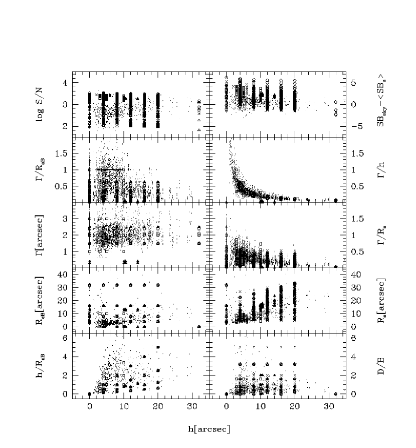
Figure 1: The parameter space of the $R^{1/4}$ plus exponential profile of the Monte Carlo simulations discussed in Figure 2-11. Models of Figs. 2-7: crosses (see also Table 2). Models of Fig. 8: skeletal triangles. Models of Fig. 9: open triangles. Models of Figs. 10-11: open squares. Models of Fig. 12: open pentagons. Models of Fig. 13: open hexagons. The small dots show the position of the EFAR galaxies as determined in Paper 3. The parameters of bulge only models are shown with $h=0$. The parameters of disk only models are shown at $R_{eB}=0$. See discussion in §3.

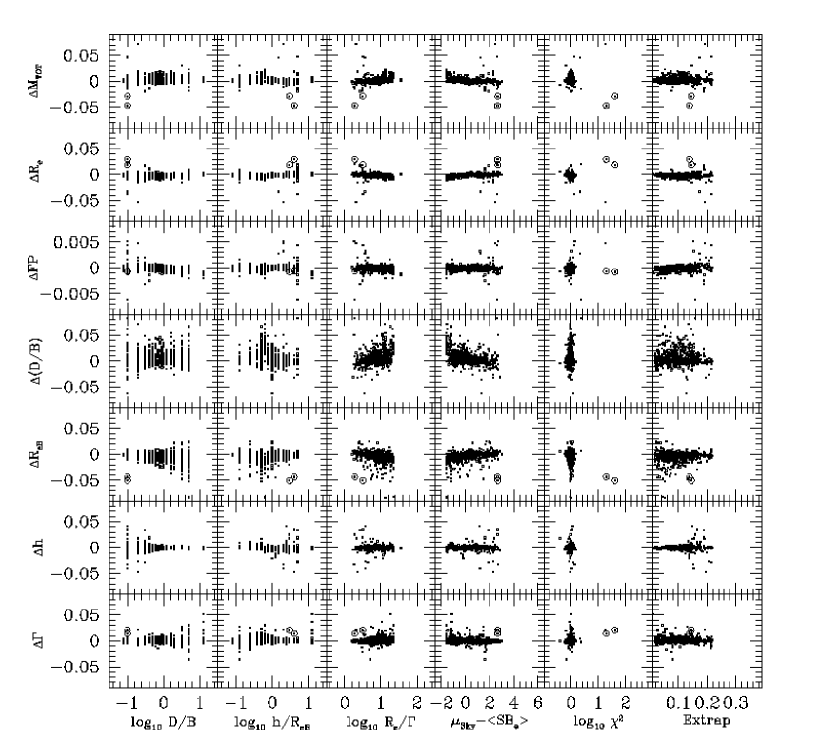
Figure 2: The reconstructed parameter space for the models indicated by the crosses in Fig. 1. No sky error is present. The quantities plotted on the y-axis are defined as $\Delta M_{TOT}=M_{TOT}-M_{TOT}^{f}$, $\Delta R_{e}=\log R_{e}/R_{e}^{f}$, $\Delta FP=\Delta R_{e}-0.3(\Delta M_{TOT}+5\Delta R_{e})=\Delta R_{e}-0.3\Delta\langle SB_{e}\rangle$, $\Delta(D/B)=\log[(D/B)/(D/B)^{f}$], $\Delta R_{eB}=\log R_{eB}/R_{eB}^{f}$, $\Delta h=\log h/h^{f}$, $\Delta\Gamma=\log\Gamma/\Gamma^{f}$. On the x-axis, the first three boxes show the input parameters of the models in the logarithm units ($\log D/B$, $\log h/R_{eB}$, $\log R_{e}/\Gamma$). The last three boxes show the differences in magnitudes between the assumed sky value and the average effective surface brightness of the models ($\mu_{\hbox{\rm Sky}}-\langle SB_{e}\rangle$), the logarithm of the reduced $\chi^{2}$, and the fraction of light extrapolated beyond $R_{max}$ used in the determination of $M^{f}_{TOT}$. Models with $D/B=0$ (pure $R^{1/4}$ laws) are plotted at $\log D/B=-1.1$ and $\log h/R_{eB}=-1.1$. Models with $B/D=0$ (pure exponential laws) are plotted at $\log D/B=1.1$ and $\log h/R_{eB}=1.1$. Models with $D/B\neq 0$ which have been fitted with one component are circled. See §3.1 for a discussion of the results.

Figure 3: (a) A circular disk plus bulge model with $D/B=0.1$ and $h/R_{eB}=5$ (crosses). The dotted curves show the luminosity profiles $\mu(R)=-2.5\log I(R)$ of the bulge and the disk components, the dashed curve the fitted disk component. (b) The differences $\Delta\mu$ (in mag arcsec^-2, open squares) between model surface brightness and the fitted one (dotted curve) (see §3.1). (c) The $R^{1/4}$ fit (solid curve) to the surface brightness magnitude profile of a circular disk plus bulge model with $D/B=0.8$ and $h/R_{eB}=1$ (crosses, one point in every four). (d) The differences $\Delta mag$ between the $R^{1/4}$ integrated magnitudes and the fitted ones (solid curve, see §3.1). Note that $|\Delta mag|<0.07$ even if large deviations $\Delta\mu$ are present. (e) The fit to the circularized profile of a flattened bulge plus an inclined disk model (see §. 3.7). The luminosity profile of the model (crosses, one point in every four; the bulge and the disk components, with the listed parameters, are the full curves) is best fitted by an $R^{1/4}$ plus exponential law (dashed curves) with parameters $R_{eB}^{f}=16.34$ arcsec, $h^{f}=13.93$ arcsec, $(D/B)^{f}=0.13$, $R_{e}=17.51$ arcsec. (f) The residuals $\Delta\mu$ of the fit (open squares, one point in every four) and the differences between the growth curves $\Delta mag$ (full curve).

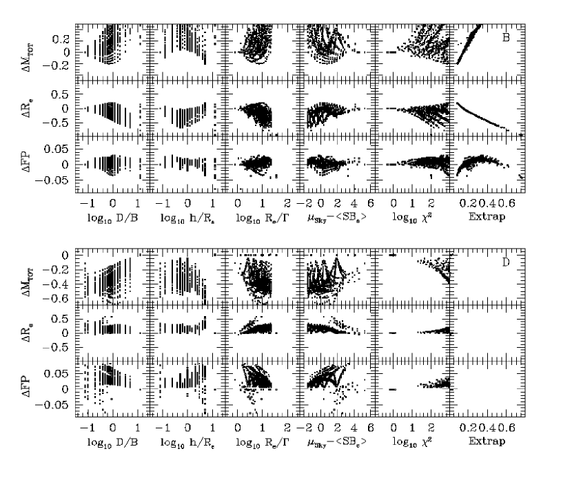
Figure 4: The effects of fitting disk plus bulge test profiles by either a single bulge (first three rows of plots) or a single disk (last three rows of plots) model. The test models are indicated by the crosses of Fig. 1. $\Delta M_{TOT}$, $\Delta R_{e}$, and $\Delta FP$ are defined as in Fig. 2, x-axis as in Fig. 2. See §3.1 for the a discussion of the results. Note the change of scale on the ordinate axis with respect to Figure 2.

Figure 5: Illustration of the underestimation of the errors. The contours of constant $\chi^{2}$ near the minimum of an $R^{1/4}$ fit to a $h/R_{eB}=0.5$, $D/B=0.1$ disk plus bulge model. The cross shows the best-fit solution, the circle near the upper left corner gives the real parameters of the model. The errors estimated at the $5\sigma$ contour underestimate the differences between the model and the fit by a factor 2 (see §3.1).

3.2 Sky subtraction errors

Sky subtraction errors can induce severe systematic errors on the derived photometric parameters of galaxies. Figure 6 shows the parameters derived from the $R^{1/4}$ plus exponential models examined in the previous section, where now the sky has been overestimated or underestimated by $\pm 1$%. The sky correction algorithm is not activated.

The biases become increasingly large as the sky brightness approaches the effective surface brightness of the models. As expected, underestimating the sky (a negative sky error) produces total magnitudes that are too bright and half-luminosity radii that are too large relative to the true ones. The size of the bias correlates with the extrapolation needed to derive $M_{TOT}^{f}$. The opposite happens when the sky is overestimated, but the amplitude of the bias is smaller, because there is no extrapolation. The correlated error $\Delta FP$ remains small ($\approx 0.05$), except for the cases where large extrapolations are involved. The D/B ratio is ill determined, with better precision for models with extended disks ($h/R_{eB}>2.5$). The scale length of the bulge is better determined for low values of $D/B$ (dominant bulge), the scale length of the disk component is better determined for large values of $D/B$ (dominant disk). The parameter least affected is the value $\Gamma$ of the seeing, which is determined in the inner, bright parts of the models, where sky subtraction errors are unimportant. Bulge-only or disk-only models appear to be fit best by two-component models (crosses and triangular crosses in Figure 6). Finally, note that reasonably good fits ($\chi^{2}<10$) to the surface brightness profiles are always obtained, in spite of the large errors on the reconstructed parameters.

The biases discussed above can be fully corrected when the sky-fitting algorithm of Eq. 12 is applied. Figure 7 shows the reconstructed parameters of the models considered in §3.1, where sky subtraction errors of 0, $\pm 1$%, $\pm 3$% have been introduced. For most of the models examined, the errors on the derived quantities are no more than a factor 2 larger than those shown in Fig. 2. The sky corrections are computed to better than 0.5% precision. Larger errors $\Delta M_{TOT}$ and $\Delta R_{e}$ are obtained for models with relatively weak ($D/B<0.3$) and extended disks ($h/R_{eB}>2.5$), where the degeneracy discussed in §3.1 is complicated by the sky subtraction correction. These cases give reasonably good fits ($\chi^{2}<10$), but are identified by the large extrapolation ($>0.3$) involved. Models with concentrated disks ($h/R_{eB}<0.2$) can also be difficult to reconstruct, when $h/\Gamma\approx 1$. For some of these problematic fits, one-component solutions are preferred by Eqs. 13-14 (circles in Eq. 7).

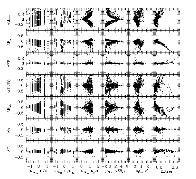
Figure 6: The biases introduced by a $\pm 1$% sky subtraction error. Quantities plotted as in Fig. 2. Models with $D/B=0$ which have been fitted with two components are shown as crosses. Models with $B/D=0$ which have been fitted with two components are shown as triangular crosses. Note the change of scale on the ordinate axis with respect to Figure 2. See discussion in §3.2.

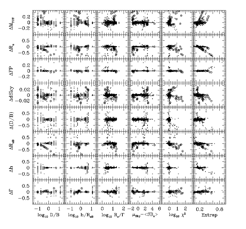
Figure 7: The effects of the sky fitting algorithm. The parameters of the models of Fig. 6 with the sky subtraction errors of 0, $\pm 1$%, $\pm 3$%, are reconstructed using the sky fitting algorithm. Quantities and symbols plotted as in Figures 2 and 6. In addition, the difference $\Delta$dSky=dSky/Sky-dSky${}^{f}/$Sky on the sky correction is plotted. Note the change of scale on the ordinate axis with respect to Figure 2. See discussion in §3.2.

A common problem of CCD galaxy photometry is the relatively small field of view, particularly with the older smaller CCDs. If the size (projected on the sky) of the CCD is not large enough compared to the half-luminosity radius of the imaged galaxy, then the sky as determined on the same frame will be contaminated by galaxy light and biased to values larger than the true one. Total magnitudes and half-luminosity radii can therefore be biased to smaller values, the effect being more important for intrinsically large galaxies, which tend to have low effective surface brightnesses. The mean surface brightness in the annulus with radii $R_{i}^{max}$ and $2R_{i}^{max}$ (see §2.2) predicted by the fit allows us to estimate the size of the contamination.

3.3 Radial extent

Photoelectric photometry of large, nearby galaxies rarely goes beyond 1 or 2 $R_{e}$ (Burstein et al. 1987) and the same applies for the surface photometry obtained with smallish CCDs. The typical profiles obtained in Paper III extend to a least 4 $R_{e}$, but a small fraction of them are less deep, reaching 1 or 2 $R_{e}$ only. Here we investigate the effect of the radial extent of the profiles, keeping the normalization of the profiles fixed ($10^{7}$ counts, $S/N\approx 10^{3}$). Sky subtraction errors of $0$, $\pm 3$% are introduced and the sky fitting is activated. Figure 8 shows the cumulative distributions of the errors on the derived photometric parameters as derived from the simulations, for a range of $R_{max}$ values. When $R_{max}=R_{e}$, rather large errors are possible (0.3 mag in the total magnitude, $>30$% in $R_{e}^{f}$). The main source of error is again the large extrapolation involved when $R_{max}\approx R_{e}$, coupled with the sky correction which becomes unreliable for these short radial extents. As soon as $R_{max}\geq 3R_{e}$ the errors reduce to the ones discussed in §3.1. The same kind of trend is observed for the parameters of the two component ($\Delta(D/B)$, $\Delta R_{eB}$, $\Delta h$). The seeing values are less affected, as they are sensitive to the central parts of the profiles only. Finally, note that in all cases very good fits are obtained ($\chi^{2}\approx 1$).

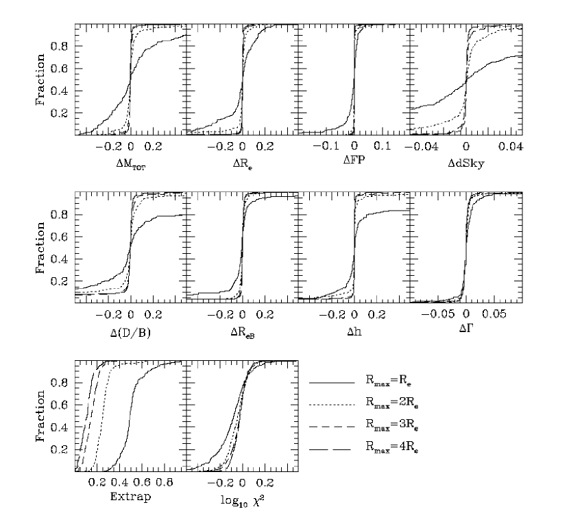
Figure 8: The effect of the radial extent of the profiles on the precision of the derived parameters. The cumulative distributions of the errors on the derived photometric parameters as derived from the simulations are shown for a range of $R_{max}$ values (full lines: $R_{max}=R_{e}$, dotted lines: $R_{max}=2R_{e}$, dashed lines $R_{max}=3R_{e}$, long-dashed lines: $R_{max}=4R_{e}$). Good reconstructions are obtained when $R_{max}/R_{e}>2$ (see §3.3).

3.4 Signal-to-noise ratio

For most of the galaxies discussed in Paper III, multiple profiles are available with integrated signal-to-noise ratios $S/N>300$, the normalization used in the previous sections. But for some of the luminosity profiles a smaller number of total counts has been collected (see Figure 1). Here we investigate how the signal-to-noise ratio of the profiles affects the outcome of the fits. As before, the subset of models of §3.2 is used with $R_{max}\leq 4R_{e}$ (see comment at the beginning of §3). Sky subtraction errors of $0$, $\pm 3$% are introduced and the sky fitting is activated. Figure 9 shows how the errors on the derived parameters increase when the signal-to-noise ratio is reduced. For fluxes as low as about $10^{5}$ ($S/N\approx 10^{2}$) all of the derived photometric parameters become uncertain (0.2 mag in the total magnitudes, 20% variations in the derived $R_{e}$, large spread $\Delta(D/B)$, $\Delta R_{eB}$, $\Delta h$, $\Delta\Gamma$), as large extrapolations and uncertain sky corrections are applied. In all cases very good fits are obtained ($\chi^{2}\approx 1$).

Figure 9: The effect of the signal-to-noise ratio of the profiles on the precision of the derived parameters. Good reconstructions are obtained when $S/N>300$ (see §3.4). Note the change of scale on the ordinate axis with respect to Figure 2.

3.5 Seeing and sampling effects

Some of the galaxies considered in Paper III are rather small, with $R_{e}<4^{\prime\prime}$. Here we investigate the effects of seeing and pixel sampling, when $R_{e}\approx\Gamma\approx$pixel size. Figure 10 shows that reliable parameters can be derived down to $R_{e}\approx\Gamma$, with pixel sizes 0.4-0.8 arcsec, with only a small increase of the scatter for $R_{e}<2\Gamma$.

A small systematic effect is caused by the choice of the psf. Saglia et al. (1993) demonstrate that a good approximation of the psfs observed during the runs described in Paper III is given by the $\gamma$ psf with $\gamma=1.5-1.7$. We adopt $\gamma=1.6$ for the fits. Here we test the effect of having $\gamma=1.5$ or 1.7 with a pixel size of 0.8 arcsec. Figure 11 shows that if $\gamma=1.5$ is the true psf of the observations, then the half-luminosity radius, the total luminosity, the scale length of the bulge will be slightly overestimated, and the disk to bulge ratio slightly underestimated. A small systematic trend is observed in the correlated errors $\Delta FP$. The scale length of the disk component is less affected. The sky corrections are also biased, but do not strongly affect the photometric parameters, because of the high average surface brightness of the small $R_{e}$ models. Seeing values suffer a very small, but systematic effect. The opposite trends are observed if the true $\gamma$ is 1.7. In all cases very good fits are obtained ($\chi^{2}\approx 1$). The systematic differences become unimportant for $R_{e}>2\Gamma$.

Finally, the seeing values derived can be systematically biased, if the central concentration of the fitted galaxies does not match the one of the $R^{1/4}$ plus exponential models. We investigate this effect by fitting the $\Psi=12$ plus exponential or the smoothed $R^{1/4}$ plus exponential models discussed in §2.2. We find that in the first case the seeing value is underestimated which compensates for the higher concentration of the $\Psi=12$ component. The shallow radial decline of the luminosity profile in the outer parts introduces systematic biases in the reconstructed parameters, similar to those discussed for the $R^{1/n}$ profiles, for large values of $n$ (see §3.8). The half-luminosity radii and total magnitudes derived are underestimated by 20% and 0.2 mag respectively, when a $\Psi=12$ model with no exponential component is fitted. The biases are reduced when models with an exponential component are constructed. In the case of the smoothed $R^{1/4}$ law, the seeing value is overestimated to fit the lower concentration of the smoothed $R^{1/4}$ component. No biases are introduced on the other reconstructed parameters.

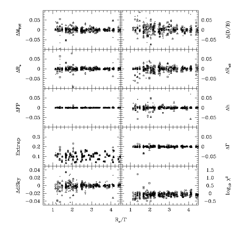
Figure 10: The effect of seeing and pixel sampling of the profiles on the precision of the derived parameters. Different symbols indicate different pixel sizes (small dot 0.4 arcsec, triangles 0.6 arcsec, squares 0.8 arcsec). Note the expanded ordinate scale with respect to Figures 4-9. See discussion in §3.5.

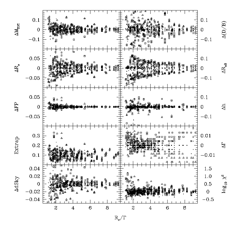
Figure 11: The effect of the choice of the psf on the precision of the derived parameters. Open triangles for $\gamma=1.5$, dots for $\gamma=1.6$ and open squares for $\gamma=1.7$. Fits performed with the $\gamma=1.6$ psf overestimate (underestimate) magnitudes and half-luminosity radii of models constructed with $\gamma=1.5$ ($\gamma=1.7$; see §3.5). Note the expanded ordinate scale with respect to Figures 4-9.

3.6 Tests of profile combination

In order to test the combination algorithm described in 2.1, four profiles with different $\Gamma$, pixel sizes, normalizations, gain, readout noise, and sky subtraction errors (see Table 3; these parameters match the typical values of the profiles of Paper III) are generated for the set of models identified by the open pentagons of Figure 1. Figure 12 shows the result of the test. The abscissa plots the residuals $\Delta$ of the parameters derived using the fitting procedure with profile combination. $\Delta$ dSky and $\Delta\Gamma$ are averaged over the four obtained values. The ordinate plots the mean of the residuals of the parameters derived by fitting each single independently as crosses, and the residuals of each fit as dots. The profile combination algorithm obtains better precision on all of the parameters with the exception of $\Gamma$, where the maximum deviation is in any case smaller than 8%.

Figure 12: The profile combination algorithm and the precision of the derived parameters. The x-axis plots the residuals $\Delta$ of the parameters derived using the fitting procedure with profile combination. $\Delta$ dSky and $\Delta\Gamma$ are averaged over the four obtained values. The y-axis plots the mean of the residuals of the parameters derived by fitting each single independently as crosses, and the residuals of each fit as dots (see discussion in §3.6).

Table 3: The parameters of the multiple profiles test (see §3.6).

Profile	1	2	3	4
Pixel size $(^{\prime\prime})$	0.4	0.606	0.862	0.792
Sky per pixel	300	350	250	1500
$\delta$Sky/Sky	$+1$%	$-0.5$%	$+1.5$%	$+0.5$%
$R_{max}/R_{e}$	4	3	4.5	2.5
Normalization	$10^{7}$	$5\times 10^{6}$	$10^{7}$	$5\times 10^{6}$
Gain	1	3	1	2
Ron	1	4	1	5
$\Gamma(^{\prime\prime})$	2	2.1	1.5	2.4

3.7 “Bulge” and “Disk” components

The discussion of the previous sections shows that for a large fraction of the parameter space, i.e. when deep enough profiles are available, with large enough objects, not only can the global photometric parameters $R_{e}$ and $M_{TOT}$ be reconstructed with high accuracy, but also the parameters of the $R^{1/4}$ and the exponential components. Here we investigate further if reliable “bulge” and “disk” parameters can be derived, when the profiles analysed are constructed from the superposition of these two components.

With this purpose, we constructed a number of two-dimensional frames (filled triangles in Figure 1) as the sum of a flattened $R^{1/4}$ bulge and an exponential disk of given inclination. The bulge (disk) frames follow an exact $R^{1/4}$ (exponential) law with $R_{eB}=12\sqrt{b/a}$ arcsec ($h=10\sqrt{\cos(i)}$ arcsec) along the minor axis. Three flattenings of the bulge ($b/a=1,0.7,0.4$), four inclinations for the disk ($i=0^{\circ},30^{\circ},60^{\circ},80^{\circ}$, where $i=0^{\circ}$ is face-on and $i=90^{\circ}$ edge-on) and five values of the disk to bulge ratio ($D/B=0,0.5,1,2,\infty$) are considered. The resulting models are normalized to $10^{7}$ counts. The pixel size is 0.6 arcsec. The circularly averaged luminosity profiles are derived following the same procedure adopted for the observed galaxies (see Paper III) and extend out to $\approx 4-6R_{e}$. A 1% sky error is introduced and the sky fitting procedure is activated. Note that the maximum flattening of the EFAR galaxies is $b/a=0.5$, with 96% of the galaxies having $b/a>0.6$ (see Paper III). This corresponds to (pure) disk inclinations $i\leq 60^{\circ}$.

Figure 13 shows the reconstructed parameters as a function of the inclination angle of the disk, for the different flattenings of the bulge, using the sky fitting procedure. The horizontal bars show models with $D/B=0.5$. The plot at the bottom right shows the scale lengths of the flattened bulge (filled symbols) or of the inclined disk as a function of the flattening angle (open symbols, $i=arccos(b/a)$) or of the inclination angle, normalized to the $b/a=1$ or $i=0^{\circ}$ values. When $D/B$ is low ($\leq 0.5$) the errors are very small for every inclination angle. For larger values of $D/B$, reliable photometric parameters are obtained for $i<60^{\circ}$, but as soon as the disk is nearly edge-on, total magnitudes and half-luminosity radii are overestimated (by 0.1 mag and 20% respectively). The integrated circularized profiles, in fact, converge more slowly than the ones following the isophotes. The correlated errors $\Delta FP$ always remain very small. Similarly, the parameters of the two components are reconstructed well for $i<60^{\circ}$, but badly underestimate the disk when it is nearly edge-on. However, a decent fit is obtained, by increasing the half-luminosity radius of the bulge component (see Fig. 3 (e) and (f)). The sky correction is returned to better than 0.5% for $i<80^{\circ}$. The systematic effects connected to the flattening of the bulge are small for the range of ellipticities considered here ($b/a\geq 0.6$).

These results indicate two potential problems, (i) galaxies may be misclassified due to the presence of an edge-on disk component not being recognized, or (ii) the photometric parameters may be systematically overestimated. However, these problems do not apply to the EFAR sample, where $b/a>0.5$ always and $b/a\geq 0.6$ for 96% of the galaxies. Therefore, galaxies with bright edge-on disks are only a very small fraction. Galaxies with faint edge-on disks, which may not show large averaged flattenings, have low $D/B$ ratios and therefore are not affected by problem (ii). In a future paper we will address the question whether in these cases the isophote shape analysis might detect these faints disks and improve on point (i).

Finally, the two-dimensional frames described here have been used to calibrate the estimator of the galaxy light contamination described in §2.2. We measured the sky in the same way as for the real frames of Paper III, by considering some small areas around the simulated galaxies. We find that the predicted galaxy light contamination overestimates the measured sky excess by at least a factor two, and therefore can be used as a rather robust upper limit to the galaxy light contamination.

Figure 13: The reconstructed parameters of the bulge plus disk models as a function of the inclination $i$ of the disk. Different symbols indicate different flattenings of the bulge. The horizontal bars show models with $D/B=0.5$. The plot at the bottom right shows the scale lengths of the flattened bulge (open symbols) or of the inclined disk (filled symbols) as a function of the flattening angle ($i=arccos(b/a)$) or of the inclination angle, normalized to the $b/a=1$ or $i=0^{\circ}$ values. Good reconstructions of the parameters are obtained when the inclination is less than $60^{\circ}$ (see §3.7).

3.8 $R^{1/n}$ luminosity profiles

The tests described above show that our fitting algorithm is able to reconstruct the parameters of a sum of an $R^{1/4}$ plus an exponential law accurately. In these cases sky subtraction errors can also be corrected efficiently. Even so, we do find in Paper III that luminosity profiles of real early-type galaxies show systematic differences from $R^{1/4}$ plus exponential profiles, yielding to a median reduced $\chi^{2}$ of 6. Here we quantify the systematic effects that would be produced in this case, by studying the case of the $R^{1/n}$ profiles.

CCO fitted the luminosity profiles of 52 early-type galaxies using the $R^{1/n}$ law introduced by Sersic (1968):

$$I(R)=I_{e}^{n}10^{-b_{n}\left[\left(\frac{R}{R_{e}^{n}}\right)^{1/n}-1\right]},$$ (16)

where $b_{n}\approx 0.868n-0.142$, $R_{e}^{n}$ is the half-luminosity radius, and $I_{e}^{n}$ the surface brightness at $R_{e}^{n}$. The total luminosity is $L_{T}=K_{n}I_{e}^{n}{R_{e}^{n}}^{2}$, where $\log K_{n}\approx 0.03[\log(n)]^{2}+0.441\log(n)+1.079$. Eq. 16 reduces to Eq. A1 for $n=4$ and to Eq. A2 for $n=1$. For large values of $n$, Eq. 16 describes a luminosity profile which is very peaked near the center and has a very shallow decline in the outer parts. Ciotti (1991) computes the curve of growth related to Eq. 16 analytically for integer values of $n$ and finds that while already $\approx 13$% of the total light is included inside $R<0.05R_{e}^{n}$, only 80% of the total light is included inside $6R_{e}^{n}$ for $n=10$.

We fitted Eq. 16, modified to have a core at $R<0.05R_{e}^{n}$, to an $R^{1/4}$ plus exponential model for $n=0.5$ to $n=15$ out to $6R_{e}^{n}$. Fig. 14 shows the results of the fit for a selection of models. With the exception of the $n=0.5$ model, all of the $R^{1/n}$ profiles can be described by a combination of an $R^{1/4}$ and an exponential component, with residuals less than 0.2 mag arcsec^-2 for $R\leq 4R_{e}$. For $n<4$ the residuals increase to 0.4 mag arcsec^-2 at $R>5R_{e}^{n}$, where the fits are increasingly brighter than the $R^{1/n}$ profiles. For large values of $n$ the residuals reach -0.4 mag arcsec^-2 at $R>5R_{e}^{n}$, where the fits are increasingly fainter than the $R^{1/n}$ profiles. The relation between $n$ and the parameters of the decomposition is shown in Fig. 15. Models with $1<n<4$ are fitted using a decreasing amount of the exponential component, with a scale length comparable to the one of the $R^{1/4}$ component. Models with $n>4$ are fitted with an increasing amount of the exponential component, with increasingly large scale length. Half-luminosity radii are progressively underestimated, being $\approx 60$% of the true values at $n=15$. Correspondingly, total magnitudes are also underestimated, by 0.25 magnitudes at $n=15$.

A possible problem can emerge for large values of $n$, if the sky fitting algorithm is activated. The dotted curves in Fig. 15 show that if the sky subtraction algorithm is activated (Eq. 12), then larger systematic effects are produced. Note that the computed sky correction (dotted curve of Fig. 15) is $\approx 0$ for $n\approx 1$ or $n\approx 4$ only. For $n>4$ the correction is used to reduce the systematic negative differences in the outer parts of the profiles. A comparison between the fitted sky corrections and the upper limits on the possible galaxy light contamination (see §2.2 and 3.7) gives an important consistency check. In the case shown in Fig. 15 the fitted sky corrections are twice as large as the upper limits on the galaxy light contamination. In a real case this, together with the rather large values of $\chi^{2}$, would hint at an uncertain fitted sky correction.

The fact that the $R^{1/n}$ sequence can be approximated by a subsample of $R^{1/4}$ plus exponential models suggests a possible reinterpretation of CCO’s results: the variety of profile shapes of early-type galaxies is caused by the presence of a disk component. Moreover, the use of the $R^{1/n}$ profiles to determine the photometric parameters of galaxies of large $n$ is dangerous, since the extrapolation involved is large and the fitted profiles barely reach 2 or 3$R_{e}^{n}$, as derived from the fit. This problem is much smaller using the $R^{1/4}$ plus exponential approach.

Figure 14: The fits to the $R^{1/n}$ law. Two plots are drawn for each value of $n$ (given in the top right corner). In the top plot the crosses (one point in every seven) show the luminosity profiles $\mu(R)=-2.5\log I(R)$ of the $R^{1/n}$ law as a function of $R/R_{e}$. The dotted and dashed curves show the best-fitting $R^{1/4}$ and exponential laws respectively. In the bottom plot the residuals (full curves) in mag arcsec^-2 from the fits to the $R^{1/n}$ law are shown. The dashed curve shows the residuals (in mag) from the curves of growth (see discussion in §3.8).

Figure 15: The relation between $n$ and the parameters of the decomposition (see §3.8). The full curves refer to the results obtained with no sky subtraction errors. The dotted curves show the results obtained when the sky fitting algorithm is activated.

3.9 Discussion

We conclude our tests by discussing the quality parameters defined in Table 1 and their use to estimate the size of the systematic errors present.

The definitions given in Table 1 have been derived after inspection of Figures 2 to 15, with the desired goal of identifying three classes of precision, $\Delta M_{TOT}\leq 0.05$, $\Delta M_{TOT}\leq 0.15$, $\Delta M_{TOT}>0.15$. The parameters $Q_{E}$, $Q_{max}$, $Q_{\chi^{2}}$, $Q_{S/N}$, and $Q_{\Gamma}$ are directly related to the simulations. Their low values imply that the fits involve a small extrapolation, extend to large enough radii, give low surface brightness residuals with a large enough signal-to-noise ratio and good spatial resolution. The definitions of $Q_{\hbox{Sky}}$ and $Q_{\delta\hbox{Sky}}$ deal with the accuracy of the sky subtraction, taking into account that high surface brightness galaxies suffer less from this problem, and that large sky corrections indicate a lower quality of the data. Low values of $Q$ (see Eq. 15) imply low values of all quality parameters.

Figure 16 shows the cumulative distributions of the errors $\Delta M_{TOT}$, $\Delta R_{e}$ and $\Delta FP$ derived from all the performed disk plus bulge fits with sky correction algorithm activated, as a function of the different quality parameters. The two most important parameters regulating the precision of the photometric parameters are the level of extrapolation and the goodness of the fit, followed by the sky subtraction errors. A low $Q_{E}$ fixes the maximum possible overestimate of the parameters. A low $Q_{\chi^{2}}$ with a low $Q_{E}$ constrains the underestimate and the reliability of the sky correction. The ranges of the errors match the desired goal of identify three classes of precisions.

Finally, it is sobering to note that the constraints needed to achieve $Q=1$, high precision total magnitudes and $R_{e}$ are rather stringent. Only 16% of EFAR galaxies have $Q=1$. Most of the existing published values of $M_{TOT}$ and $R_{e}$ of galaxies are far below this precision, because of the restricted radial range probed by photoelectric measurements or small CCD chips, because of sky subtraction errors, and also by the use of the pure $R^{1/4}$ curve of growth fitting (see Figure 4). The related observational problems can be somewhat reduced with the use of large CCDs (see Introduction), but the a priori limiting factor of galaxy photometry, the extrapolation, will always remain with us at a certain level.

On the other hand, the errors on $M_{TOT}$ and $R_{e}$ are strongly correlated, so that the quantity $\log R_{e}-0.3\langle SB_{e}\rangle$ is always well determined. This fact allows the accurate distance determinations achieved using the Fundamental Plane correlations despite the systematic errors in the photometric quantities.

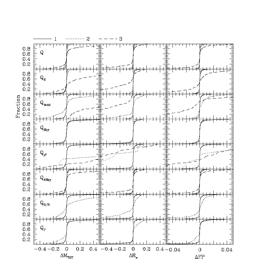
Figure 16: The precision of the reconstructed total magnitudes $M_{TOT}$, the half-luminosity radii $R_{e}$ and the combined quantity $FP=\log R_{e}-0.3\langle SB_{e}\rangle$. The cumulative distributions of the errors $\Delta M_{TOT}$, $\Delta R_{e}$ and $\Delta FP$ derived from all the performed disk plus bulge fits with sky correction algorithm activated are shown as a function of the different quality parameters defined in §2.3. The full lines plot the distributions when the parameters have value of 1, the dotted ones when the value is 2, the dashed ones when the value is 3. The distributions derived by selecting on the global quality parameter $Q$ match the precision ranges identified in §3.9.

4 Conclusions

We constructed an algorithm to fit the circularized profiles of the (early-type) galaxies of the EFAR project, using a sum of a seeing-convolved $R^{1/4}$ and an exponential law. This choice allows us to fit the large variety of profiles exhibited by the EFAR galaxies homogeneously. The procedure provides for an optimal combination of multiple profiles. A sky fitting option has been developed. A conservative upper limit to the sky contamination due to the light of the outer parts of the galaxies is estimated. From the tests described in previous sections we draw the following conclusions:

1) The reconstruction algorithm applied to simulated $R^{1/4}$ plus exponential profiles shows that random errors are negligible if the total signal-to-noise ratio of the profiles exceeds $300$. Systematic errors due to the radial extent of the profiles are minimal if $R_{max}/R_{e}>2$. Systematic errors due to sky subtraction are significant (easily larger than 0.2 mag in the total magnitude) when the sky surface brightness is of the order of the average effective surface brightness of the galaxy. They can be reliably corrected for as long as the fitted profiles show small systematic deviations ($\chi^{2}<12.5$).

2) Strong systematic biases (errors larger than 0.2 mag in the total magnitudes) are present when a simple $R^{1/4}$ or exponential model is used to fit test profiles with disk to bulge ratios as low as 0.2.

3) The use of the shape of the (normalized) $\chi^{2}$ function badly underestimates the (systematic) errors on the photometric parameters.

4) Systematic biases emerge when test profiles are derived for systems with significant disk components seen nearly edge-on, or when the fitted luminosity profile declines more slowly than an $R^{1/4}$ law. The parameters of bulge plus disk systems can be determined to better than $\approx 20$% if the disk is not very inclined ($i<60^{\circ}$).

5) The sequence of $R^{1/n}$ profiles, recently used to fit the profiles of elliptical galaxies by Caon et al. (1993), is equivalent to a subset of $R^{1/4}$ and exponential profiles, with appropriate scale lengths and disk-to-bulge ratios, with moderate systematic biases for $n\leq 8$ and residuals less than 0.2 mag arcsec^-2 for $R\leq 4R_{e}$. This suggests that the variety of luminosity profiles shown by early-type galaxies is due to the frequent presence of a weak disk component.

6) A set of quality parameters has been defined to control the precision of the estimated photometric parameters. They take into account the amount of extrapolation involved to derive the total magnitudes, the size of the sky correction, the average surface brightness of the galaxy relative to the sky, the radial extent of the profile, its signal-to-noise ratio, the seeing value and the reduced $\chi^{2}$ of the fit. These are combined into a single quality parameter $Q$ which correlates with the expected precision of the fits. Errors in total magnitudes $M_{TOT}$ less than 0.05 mag and in half-luminosity radii $R_{e}$ less than 10% are expected if $Q=1$, and less than 0.15 mag and 25% if $Q=2$.

89% of the EFAR galaxies have fits with $Q=1$ or $Q=2$. The errors on the combined Fundamental Plane quantity $FP=\log R_{e}-0.3\langle SB_{e}\rangle$, where $\langle SB_{e}\rangle$ is the average effective surface brightness, are smaller than 0.03 even if $Q=3$. Thus systematic errors on $M_{TOT}$ and $R_{e}$ only marginally affect the distance estimates which involve $FP$.

Appendix A The fitting function

The fitting procedure described in §2 assumes that fitted profiles can be well represented by the sum of a de Vaucouleurs (1948) law of half-luminosity radius $R_{eB}$ and a surface brightness $I_{eB}$ at $R_{eB}$ (with $B$ for bulge component):

$$I_{B}(R)=I_{eB}\exp\{-7.67[(R/R_{eB})^{1/4}-1]\},$$ (A1)

and an exponential component with exponential scale-length $h$ and central surface brightness $I_{0}$ (with $D$ for disk component):

$$I_{D}(R)=I_{0}\exp(-R/h).$$ (A2)

The $R^{1/4}$ law curve-of-growth is:

$$F_{B}(R)=L_{B}\left[1-\exp(-z)\left(1+\sum_{n=1}^{7}\frac{z^{n}}{n!}\right)\right],$$ (A3)

where the total luminosity of the bulge component is normalized, $L_{B}=7.22\pi I_{eB}R_{eB}^{2}=1$, and $z=7.67(R/R_{eB})^{1/4}$. The exponential law curve-of-growth is:

$$F_{D}(R)=L_{D}[1-(1+R/h)\exp(-R/h)],$$ (A4)

where the total luminosity of the disk component is set to the disk-to-bulge ratio, $L_{D}=2\pi I_{0}h^{2}=(D/B)$, if a two-component model is considered, or normalized, $L_{D}=1$, if an exponential only model is used (in this case $L_{B}=0$).

Both laws are seeing convolved with a $\gamma=1.6$ psf, following the technique described by Saglia et al. (1993). The Fourier transforms of the $\gamma$ psfs are given by:

$$\hat{p}_{\gamma}(k)\equiv\int_{0}^{\infty}\,2\pi R\,J_{0}(kR)\,p_{\gamma}(R)\,dR\,=\exp[-(kb)^{\gamma}],$$ (A5)

where $J_{0}(kR)=\frac{1}{2\pi}\int_{0}^{2\pi}\exp(ikR\cos\theta)d\theta$ is the zero-order Bessel function. The $\gamma=1.6$ psf reproduces well the stellar profiles measured with the telescopes and setups used in Paper III (see Saglia et al. 1993).

A grid of seeing-convolved models is obtained for 100 values of the $\Gamma/R_{eB}$ and $\Gamma/h$ ratios, ranging from 0.01 to 1 with linear increment of 0.01. Here $\Gamma$ is the FWHM of the seeing profile. For each of these values, the seeing-convolved luminosity profiles $I^{C}_{B}(R/\Gamma,\Gamma/R_{eB})$ and $I^{C}_{D}(R/\Gamma,\Gamma/h)$ and curves of growth $F^{C}_{B}(R/\Gamma,\Gamma/R_{eB})$ and $F^{C}_{D}(R/\Gamma,\Gamma/h)$ for both the bulge and the disk component are tabulated for $0<R/\Gamma<50$ on a logarithmic radial grid (plus $R=0$) with $d\ln R/\Gamma=0.230258$ and 31 points. A cubic spline interpolation on $\ln(R/\Gamma$) and a linear interpolation on $\Gamma/R_{eB}$ or $\Gamma/h$ are used to determine the profile at a given radial distance $R$ and with given values for $R_{eB}$, $h$ and $\Gamma$. When $R/\Gamma<0.05$ a log-log extrapolation is used. When $R/\Gamma>50$ the correction computed for $R/\Gamma$=50 is applied. If $\Gamma/R_{eB}<0.01$ ($\Gamma/h<0.01$) the correction computed for $\Gamma/R_{eB}=0.01$ ($\Gamma/h=0.01$) is used. When $\Gamma/R_{eB}>1$ ($\Gamma/h>1$) the correction computed for $\Gamma/R_{eB}=1$ ($\Gamma/h=1$) is applied. The resulting numerical errors in the seeing convolved bulge and disk models are negligible ($<<1$%).

The luminosity profile $f_{B+D}=f_{B}+f_{D}$ fitted to the data takes into account the effect of the finite pixel size of the observed profiles. These are computed as the azimuthally averaged flux in the annulus of radius $R$ and of half pixel width. This procedure is reproduced by the following equations:

$$f_{B}(R,R_{eB},\Gamma,S)=\frac{1}{A}\left\{F^{C}_{B}\left[\frac{R+S/2}{\Gamma},\frac{\Gamma}{R_{eB}}\right]-F^{C}_{B}\left[\frac{R-S/2}{\Gamma},\frac{\Gamma}{R_{eB}}\right]\right\},$$ (A6)

$$f_{D}(R,h,\Gamma,S)=\frac{1}{A}\left\{F^{C}_{D}\left[\frac{R+S/2}{\Gamma},\frac{\Gamma}{h}\right]-F^{C}_{D}\left[\frac{R-S/2}{\Gamma},\frac{\Gamma}{h}\right]\right\},$$ (A7)

where $A=\pi[(R+S/2)^{2}-(R-S/2)^{2}]$ is the area of the annulus and $S$ is the scale or pixel size in arcsec. Eqs. A6 and A7 are valid for $R>S/2$. If $R<S/2$ (i.e., the central value at $R=0$), then:

$$f_{B}(R,R_{eB},\Gamma,S)=\frac{F^{C}_{B}\left[\frac{R+S/2}{\Gamma},\frac{\Gamma}{R_{eB}}\right]}{\pi(R+S/2)^{2}}$$ (A8)

$$f_{D}(R,h,\Gamma,S)=\frac{F^{C}_{D}\left[\frac{R+S/2}{\Gamma},\frac{\Gamma}{h}\right]}{\pi(R+S/2)^{2}}.$$ (A9)

Similar tables of seeing convolved profiles were also constructed for the $\Psi=12$ $f_{\infty}$ model and for the smoothed $R^{1/4}$ used in Saglia et al. (1993). The luminosity profile of the $\Psi=12$ $f_{\infty}$ model is more centrally peaked than the $R^{1/4}$ and declines less rapidly than the $R^{1/4}$ law at large radii. The smoothed $R^{1/4}$ model is less centrally concentrated than the $R^{1/4}$ law. Both profiles have been used to test our fitting algorithm (see §3.5).

References

- (1) Bender R., Döbereiner S., & Möllenhoff C. 1988, A&AS 74, 385
- (2) Bender R., & Paquet A. 1995, Proc. IAU Symp. 160, G. Gilmore, P. van der Kruit Eds.
- (3) Bender R., Saglia R.P., & Gerhard O. 1994, MNRAS, 269, 785
- (4) Burstein D., Davies R.L., Dressler A., Faber S.M., Stone R.P.S., Lynden-Bell D., Terlevich R.J., & Wegner G., 1987, ApJSS, 64, 601
- (5) Buta R., Corwin H.G.Jr., de Vaucouleurs G., de Vaucouleurs A., & Longo G., 1995, AJ, 109, 517
- (6) Byun Y.I., & Freeman K.C. 1995, ApJ 448, 563
- (7) Caon N., Capaccioli M., & D’Onofrio M., 1993, MNRAS, 265, 1013 (CCO)
- (8) Casertano S., Ratnatunga K.U., Griffiths R.E., Im M., Neuschaefer L.W., Ostrander E.J., & Windhorst R.A., 1995, ApJ, 453, 599
- (9) Ciotti L. 1991, A&A, 249, 99
- (10) Colless M., Burstein D., Wegner G., Saglia R.P., McMahan R., Davies, R.L., Bertschinger E., & Baggley G., 1993, MNRAS, 262, 475
- (11) de Jong R.S. 1996, A&A in press
- (12) de Vaucouleurs, G. 1948, Ann. d’Ap., 11, 247
- (13) de Vaucouleurs G., de Vaucouleurs, A., Corwin H.G., Buta, R.J., Paturel, G., & Fouqué, P. 1991, Third Reference Catalogue of Bright Galaxies (New York, Springer-Verlag)
- (14) de Vaucouleurs G., & Capaccioli M. 1979, ApJS 40, 699
- (15) Djorgovski S. 1985, PhD thesis, University of California, Berkeley
- (16) D’Onofrio M., Capaccioli M., & Caon N., 1994, MNRAS, 271, 523
- (17) Graham A.W. 1996, ApJ, 459, 27
- (18) Graham A.W., Lauer T., Colless M., Postman M., 1996, ApJ, 465, 534
- (19) Jørgensen I., Franx, M., & Kjærgaard P., 1995, MNRAS, 273, 1097
- (20) Kormendy J., & Djorgovski S., 1989, ARA&A, 27, 235
- (21) Lauberts A., & Valentijn E.A., 1989, “The surface photometry catalogue of the ESO-Uppsala Galaxies”, ESO, München
- (22) Lauer T. 1985, ApJ 292, 104
- (23) Lucey J.R., Guzmán R., Carter D., & Terlevich R.J. 1991, MNRAS, 253, 584
- (24) MacGillivray, H.T., Thomson E.B., Lasker B.M., Reid I.N., Malin D.F., West R.M., & Lorenz H., 1993, Proc. IAU Symp. 161, Astronomy from wide-field imaging
- (25) Metzger, M.R., Luppino, G.A., & Miyazaki, S., 1995, BAAS, 187, 7305
- (26) Michard R., 1979, A&A, 74, 206
- (27) Peletier R.F., Davies R.L., Illingworth G.D., Davis L.E., & Cawson M.C., 1990, AJ, 100, 1091
- (28) Press W.H., Flannery B.P., Teukolsky S.A., & Vetterling W.T., 1986, Numerical Recipes (Cambridge: Cambridge University Press)
- (29) Saglia R.P., Bender R., & Dressler A., 1993, A&A, 279, 75
- (30) Saglia R.P., Bertschinger E., Baggley G., Burstein D., Colless M.M., Davies R.L., McMahan R., & Wegner G., 1993 MNRAS, 264, 961
- (31) Saglia R.P., Bertschinger E., Baggley G., Burstein D., Colless M.M., Davies R.L., McMahan R., & Wegner G., 1997 in preparation (Paper III)
- (32) Scorza C., & Bender R., 1995, A&A 293, 20
- (33) Sersic J.-L., 1968, Atlas de galaxias australes, Observatorio Astronomico, Cordoba
- (34) Thomsen B., & Frandsen S. 1983, AJ 88, 789
- (35) Wegner G., Colless M., Baggley G., Davies, R.L., Bertschinger E., Burstein D., McMahan R., & Saglia R.P., 1996, ApJS , in press (Paper I)
- (36) Wegner G., Davies, R.L., Baggley G., Saglia R.P., McMahan R., Colless M., Burstein D., & Bertschinger E., 1997 in preparation (Paper II)
- (37) Windhorst R.A. et al. 1994, AJ 107, 930