QSO variability: probing the Starburst model

Abstract

The consistency of the Starburst model for AGN is tested using the optical variability observed in large data bases of QSOs. Theoretical predictions for the variability–luminosity relationship and structure function are presented and compared with observations. If QSOs follow a variability–wavelength relation as that observed in nearby AGN, the model proves successful in reproducing the main characteristics of optical variability. The wavelength dependence (1) flattens the, otherwise, monochromatic Poissonian variability–luminosity relationship; and (2) decreases the asymptotic value of the structure function, which reveals that the elementary pulse driving the variations would have a characteristic time scale of 85–280 days. The upper limit is consistent with the time scale found in nearby Seyfert galaxies. Shorter values of this time scale are expected if the metallicity of high redshift objects is high, as recent observations indicate. If distant QSOs do not follow the variability–wavelength dependence observed in Seyfert nuclei and nearby QSOs, the characteristic pulse of variation needs to be much faster in order to reproduce the variability-luminosity relationship but, then, the single-parametric model explored in this work predicts a more rapidly rising structure function than that inferred from the data.

1. Introduction

Variability is one of the most conspicuous properties of active galactic nuclei (AGN) and a potentially powerful constraint on models for these objects. In the context of the Starburst model, the variability observed in Seyfert galaxies and QSOs is produced by supernova explosions (SNe) which generate rapidly evolving compact supernova remnants (cSNRs) due to the interaction of their ejecta with the high density circumstellar environment created by their progenitor stars. During this phase, when the stellar cluster is 10–60 Myr old, the bolometric luminosity is dominated by stars, while the basic broad line region (BLR) properties can be ascribed to the evolution of cSNRs in a medium with densities $n\mathrel{\lower 2.5pt\vbox{\hbox{$>$}\hbox{$\sim$}}}10^{7}$ cm^-3 and metallicities of the order of Z_⊙ or higher (Terlevich et al. 1992). In fact, the energy and overall pattern of variability of the optical light curves of intensively monitored Seyfert nuclei, such as NGC 4151 and NGC 5548, can be well modeled by a sequence of SN and cSNR events (Aretxaga & Terlevich 1993, 1994) and the detailed response of the BLR to these variations can also be explained by the evolution of the physical properties of the structures created by the remnants (Terlevich et al. 1995), with basically just one free parameter, the density of the ambient medium. Interestingly, the values obtained for this parameter ($n\mathrel{\lower 2.5pt\vbox{\hbox{$>$}\hbox{$\sim$}}}10^{7}$ cm^-3) are also those derived from observed cSNRs, the so called “Seyfert 1 impostors”. These cSNRs present optical spectra that resemble very closely those of type 1 Seyfert nuclei and QSOs (Filippenko 1989, Stathakis & Sadler 1991, Turatto et al. 1993; see Terlevich 1994 for a review of their properties).

In the last decade, several observational studies have reported trends in the variability characteristics of optically selected quasars with either luminosity or redshift (Pica & Smith 1983, Cristiani, Vio & Andreani 1990, Giallongo, Trevese & Vagnetti 1991, Smith et al. 1993, Hawkins 1993, Hook et al. 1994; Trevese et al. 1994, Paltani & Courvoisier 1994, Cristiani et al. 1996, Di Clemente et al. 1996). Some of these studies (see for example Pica & Smith 1983) have shown that the observed anti-correlation between optical variability and QSO luminosity is somewhat flatter than a “$1/\sqrt{N}$” law, a result which seems to rule out simple Poissonian models. However, these studies disregard the fact that AGN variability is wavelength dependent. In Seyfert nuclei and low-redshift QSOs it is observed that the amplitude of the variations increases towards shorter wavelengths (Edelson, Krolik & Pike 1990, Kinney et al. 1991, Paltani & Courvoisier 1994, Di Clemente et al. 1996). Extrapolating this behaviour to high-redshift QSOs, one expects the variability measured at a fixed optical band to overestimate the monochromatic rest frame optical variability, simply because the objects are observed at bluer emitted wavelengths. Wavelength effects must be removed before analyzing the variability dependence with luminosity, and certainly before claiming that the Poissonian model is inconsistent with the data. Indeed, the parametric fits to the wavelength–luminosity–redshift relationship of QSOs performed by Cid Fernandes, Aretxaga & Terlevich (1996) show that QSO variability can be Poissonian, once wavelength effects are considered.

In this work we present the Poissonian model for the optical variability of QSOs as derived from the Starburst hypothesis, and compare it to the observations. The model makes specific predictions that are easy to check, namely, that the variability should be the result of a random superposition of events with luminosity and shape typical of cSNRs, and with a rate given by the cluster luminosity. The optical variability properties of massive stellar clusters containing cSNRs are analytically predicted in Section 2. In section 3 we use the South Galactic Pole sample of nearly 300 QSOs to test the consistency of the theoretical predictions. An analysis of wavelength–variability dependence is presented there. Monte Carlo simulations are used to reproduce the sampling and photometric uncertainties of the observations. In Section 4 we discuss the results of the modelling of the variability–luminosity relationship and structure function. Section 5 summarizes our main conclusions.

2. The variability produced by young clusters containing cSNRs

The variability generated by a Poissonian process is characterized by the following properties:

1. the rate of events;

2. the energy of the events;

3. the shape of each variation pulse, i.e. its time evolution;

4. the strength of a non-variable “background” component, if it exists.

The Starburst model makes specific predictions for each of these ingredients. In fact, we shall see that the model reduces the description of the variability properties of QSOs to a single functional parameter.

Stars and cSNRs contribute to the mean B band luminosity of a coeval stellar cluster in an approximately constant proportion during the SN II phase (10–60 Myr). This is so because both the SN rate ($\nu_{\mbox{\scriptsize SN}}$) and the optical luminosity coming from stars ($L_{\mbox{\scriptsize B}}^{\star}$) are linked to the number of massive stars present in the cluster at every moment. The ratio of these quantities is given by

$$\hbox{$\nu_{\mbox{\scriptsize SN}}$}/\hbox{$L_{\mbox{\scriptsize B}}^{\star}$}\approx 2\times 10^{-11}\mbox{ \ \ yr${}^{-1}$ \hbox{L${}_{{\mbox{\scriptsize B}}}^{\odot}$}${}^{-1}$\ \ ,}$$ (1)

almost independently of the Initial Mass Function (IMF) and age of the cluster (Aretxaga & Terlevich 1994). The number of low mass stars, which carries the bulk of the mass of the cluster, is irrelevant in this ratio. The mean total luminosity of the cluster ($\overline{\hbox{$L_{\mbox{\scriptsize B}}^{\mbox{\scriptsize clu}}$}}$) is given by the sum of the luminosity coming from stars and the mean luminosity coming from SNe ($L_{\mbox{\scriptsize B}}^{\mbox{\scriptsize SNe}}$). From expression (1), this is related to the SN rate by

$$\overline{\hbox{$L_{\mbox{\scriptsize B}}^{\mbox{\scriptsize clu}}$}}=\hbox{$L_{\mbox{\scriptsize B}}^{\star}$}+\overline{\hbox{$L_{\mbox{\scriptsize B}}^{\mbox{\scriptsize SNe}}$}}\sim 5\times 10^{10}\>\frac{\hbox{$\nu_{\mbox{\scriptsize SN}}$}}{\mbox{yr${}^{-1}$}}\>(\hbox{$\epsilon_{\mbox{\scriptsize B}}$}+1)\mbox{ \ \hbox{L${}_{{\mbox{\scriptsize B}}}^{\odot}$}\ \ \ ,}$$ (2)

where $\epsilon_{\mbox{\scriptsize B}}$ is the mean B-band energy released in each SN remnant, in units of $10^{51}$ erg. An estimation of $\epsilon_{\mbox{\scriptsize B}}$ can be obtained from the observed time averaged equivalent width of H$\beta$ (Aretxaga & Terlevich 1994),

$$\overline{\hbox{$W_{\mbox{\scriptsize H{\tiny$\beta$}}}$}}\sim 320\mbox{\AA\ \ }\frac{\hbox{$\epsilon_{\mbox{\scriptsize B}}$}}{1+0.17\hbox{$\epsilon_{\mbox{\scriptsize B}}$}}\mbox{\ \ .}$$ (3)

This expression is also independent of the age, mass or IMF of the cluster, but is weakly dependent on the adopted bolometric correction for cSNRs. Most of the optical–UV luminosity of cSNRs is emitted by dense shells of relatively cold gas formed during the remnant evolution, which reprocess a large fraction of the high energy photons generated by the fast shocks (Terlevich et al. 1992, Franco et al. 1994). The calibration of the bolometric correction was carried out using the intensities and equivalent widths of the observed cSNRs SN 1987F and SN 1988Z, giving $\hbox{$\epsilon_{\mbox{\scriptsize B}}$}/\hbox{$\epsilon_{51}$}\approx 0.12$ where $\epsilon_{51}$ is the energy emitted in B-band in units of $10^{51}$ erg. However, any systematic effect in the bolometric correction, due to metallicity or density differences, for example, could affect the energy estimation derived from expression (3). The mean equivalent width of H$\beta$ for typical QSOs is found to be $\overline{\hbox{$W_{\mbox{\scriptsize H{\tiny$\beta$}}}$}}\approx 100$ Å (Searle & Sargent 1968, Yee 1980, Shuder 1981, Osterbrock 1991), and from equation (3) the energy of cSNRs is derived to be $\hbox{$\epsilon_{\mbox{\scriptsize B}}$}\approx 0.5$ ($\hbox{$\epsilon_{51}$}\approx 4$). Values of the kinetic energy released in a SN explosion in excess of $10^{51}$ erg have been measured in recent well followed up type II SNe (Branch et al. 1981, Woosley 1988).

Figure 1: a. B band light curves of massive stellar clusters undergoing SN explosions with rates 0.1–500 yr^-1. The rates are labelled inside each panel. The time of evolution of the cSNRs used for this set of models is $t_{sg}=280$ days and the mean B-band energy is $\epsilon_{B}=0.5$. The dashed line in the panels show the luminosity level produced by the stars of the cluster (following equation (1)).

Figure 1.b. As Figure 1.a., for $t_{sg}=85$ days.

Figure 1.c. As Figure 1.a., for $t_{sg}=15$ days.

The basic element of variation in the Starburst model is generated by a SN explosion and the evolution of its associated cSNR. A simple description of such an event can be obtained through semi-analytical solutions (Shull 1980, Wheeler, Mazurek & Sivaramakrishnan 1980, Terlevich et al. 1992) as a double peak light curve given by (Aretxaga & Terlevich 1994)

$$\hbox{$L_{\mbox{\scriptsize B}}^{\mbox{\scriptsize 1SN}}$}(t)=\left\{\begin{array}[]{ll}\hskip 56.9055pt\mbox{\text@underline{\sl 1st peak: SN}}&\\ 6\times 10^{9}\hbox{L${}_{{\mbox{\scriptsize B}}}^{\odot}$}&\mbox{if $t=0$}\\ 0&\mbox{if $t=110$ days}\\ \hskip 56.9055pt\mbox{\text@underline{\sl 2nd peak: cSNR}}&\\ 0&\mbox{if $t=0.3\>\hbox{$t_{\mbox{\scriptsize sg}}$}$}\\ 3\times 10^{10}\hbox{L${}_{{\mbox{\scriptsize B}}}^{\odot}$}\>\frac{\hbox{$\epsilon_{\mbox{\scriptsize B}}$}}{\hbox{$t_{\mbox{\scriptsize sg}}$}}\left(\frac{t}{t_{\mbox{\tiny sg }}}\right)^{-11/7}&\mbox{if $t>t_{\mbox{\scriptsize sg}}$ }\end{array}\right.$$ (4)

Linear interpolation is used from the zero luminosity levels in both peaks. The zero point in the time scale corresponds to the SN outburst and $t_{\mbox{\scriptsize sg}}$ denotes the time beyond which radiative cooling becomes important in the evolution of the cSNR. For solar metallicity, $t_{\mbox{\scriptsize sg}}$ is given by (Shull 1980, Wheeler, Mazurek & Sivaramakrishnan 1980, Terlevich et al. 1992)

$$\hbox{$t_{\mbox{\scriptsize sg}}$}=0.62\mbox{\ yr \ }\hbox{$\epsilon_{51}$}^{1/8}\hbox{$n_{7}$}^{-3/4}\mbox{\ \ ,}$$ (5)

where $n_{7}$ is the circumstellar density in which the cSNR evolves, in units of $10^{7}$ cm^-3. This is a very schematic representation of the real luminosity evolution of cSNRs. Although the hydrodynamical simulations of Tenorio-Tagle and co-workers (1996) show that the overall evolution of the luminosity of a cSNR roughly follows a $t^{-11/7}$ law, several flares and fluctuations associated with shell formation, cooling instabilities and shell–shell collision occur on time scales shorter than $t_{\mbox{\scriptsize sg}}$, with energies of about $10^{49}$–$10^{50}$ erg (Terlevich et al. 1995, Plewa 1995). This general behaviour is also observed in isolated periods of activity in nearby type 1 Seyfert nuclei such as NGC 4151, NGC 5548 and NGC 1566 (Cid Fernandes, Terlevich & Aretxaga 1996, Alloin et al. 1986). These secondary flares are not included in our simplified expression of the light curve. A further approximation made in equation (4) is that the B-band bolometric correction remains constant throughout the lifetime of the cSNR.

From these expressions we can deduce that the four properties that characterize a Poissonian process can be described with just one functional parameter in the Starburst model:

1. The rate of events is linked to the total luminosity of the objects by equation (2), and also depends on the energy of the events.

2. The energy of the events in B-band is $\hbox{$\epsilon_{\mbox{\scriptsize B}}$}\approx 0.5$ in order to satisfy equation (3) with the observed values of the equivalent width of H$\beta$ in QSOs.

3. The main source of non-variable background luminosity comes from the stars in the cluster. The stellar luminosity is directly linked to the rate of events by equation (1). That makes for approximately 60 per cent of the total luminosity of the nucleus. In R-band, the host galaxies of distant ($z\approx 2$) QSOs contribute to the non-variable light with less than 18 per cent of the total luminosity of the QSOs (Aretxaga, Boyle & Terlevich 1995, Hutchings 1995), probably less in B-band. In what follows, the host galaxy contribution will be disregarded.

4. The shape of the events is given by the SN$+$cSNR light curve of equation (4), which depends on the energy ($\hbox{$\epsilon_{\mbox{\scriptsize B}}$}\approx 0.5$) and the characteristic time scale of the pulse ($t_{\mbox{\scriptsize sg}}$). This last parameter actually controls the shape of the light curve, and remains free. However, its value can be constrained to a narrow band. For Seyfert nuclei, such as NGC 4151 and NGC 5548, the values of $t_{\mbox{\scriptsize sg}}$ found to reproduce well isolated peaks in their light curves are 260–280 days (Aretxaga & Terlevich 1993,1994) but, since high luminosity QSOs may have higher metallicities (Hamann & Ferland 1992,1993), the evolution of their cSNRs could be substantially faster, as the cooling rates would increase. To allow for this effect we have set a lower limit of 15 days for $t_{\mbox{\scriptsize sg}}$.

Figures 1a,b,c show how the light curves of objects with different luminosities ($\hbox{$\overline{\hbox{$M_{\mbox{\scriptsize B}}$}}$}=-19\mbox{ to }-29$ mag) look like, depending on the adopted value of the free parameter $t_{\mbox{\scriptsize sg}}$, set to be 280, 85 or 15 days in our grid of models. To construct these model light curves of AGN, SN$+$cSNR light curves of a given $t_{\mbox{\scriptsize sg}}$ were combined at random under a certain rate, using a random number generator to determine the time of explosion. The final luminosity curve includes, in a self consistent way, the stellar luminosity as defined by relation (1). The light curves are sampled every 15 days, totaling 100 years. SNe in a given cluster may have slightly different intrinsic parameters. For instance, their circumstellar densities and/or B-band energies do not need to be exactly identical. To allow for this possibility, we have let the values of $t_{\mbox{\scriptsize sg}}$ and $\epsilon_{\mbox{\scriptsize B}}$ vary in a Gaussian way around their mean value, such that factor of $2$ variations occur within a $2\sigma$ probability.

2.1. Variability versus luminosity

The light curve statistics of one of these clusters can be analytically calculated taking into account the Poissonian nature of the SN events (Cid Fernandes 1995). The mean luminosity due to SNe and cSNRs alone is simply $\overline{\hbox{$L_{\mbox{\scriptsize B}}^{\mbox{\scriptsize SNe}}$}}=\hbox{$\nu_{\mbox{\scriptsize SN}}$}\overline{\hbox{$E_{\mbox{\scriptsize B}}$}}$, where $\overline{\hbox{$E_{\mbox{\scriptsize B}}$}}=10^{51}\overline{\hbox{$\epsilon_{\mbox{\scriptsize B}}$}}$ erg is the average B-band energy radiated by each SN$+$cSNR event. The relative standard deviation of the SNe$+$cSNRs component is given by

$$\hbox{$v_{\mbox{\scriptsize B}}^{\mbox{\scriptsize SNe}}$}\equiv\frac{\sigma(\hbox{$L_{\mbox{\scriptsize B}}^{\mbox{\scriptsize SNe}}$})}{\overline{\hbox{$L_{\mbox{\scriptsize B}}^{\mbox{\scriptsize SNe}}$}}}=\frac{1}{\left({\hbox{$\nu_{\mbox{\scriptsize SN}}$}\hbox{$\tau_{\mbox{\scriptsize B}}$}}\right)^{1/2}}\mbox{\ \ \ ,}$$ (6)

with $\tau_{\mbox{\scriptsize B}}$ being the effective lifetime of a cSNR in B-band, defined by

$$\hbox{$\tau_{\mbox{\scriptsize B}}$}\equiv\frac{\overline{\hbox{$E_{\mbox{\scriptsize B}}$}}^{2}}{\int\left\{{\int\left[{\hbox{$L_{\mbox{\scriptsize B}}^{\mbox{\scriptsize 1SN}}$}(t;\vec{x})}\right]^{2}dt}\right\}\,p(\vec{x})d\vec{x}}\mbox{\ \ \ ,}$$ (7)

where $\vec{x}$ denotes a given combination of $t_{\mbox{\scriptsize sg}}$ and $\epsilon_{\mbox{\scriptsize B}}$ and $p(\vec{x})$ is the probability density of these two parameters. For a probability distribution as that of the simulations described in the previous section and for mean values of $t_{\mbox{\scriptsize sg}}$ and $\epsilon_{\mbox{\scriptsize B}}$ in the range $15\mathrel{\lower 2.5pt\vbox{\hbox{$<$}\hbox{$\sim$}}}\hbox{$t_{\mbox{\scriptsize sg}}$}\mathrel{\lower 2.5pt\vbox{\hbox{$<$}\hbox{$\sim$}}}280$ days and $0.1\mathrel{\lower 2.5pt\vbox{\hbox{$<$}\hbox{$\sim$}}}\hbox{$\epsilon_{\mbox{\scriptsize B}}$}\mathrel{\lower 2.5pt\vbox{\hbox{$<$}\hbox{$\sim$}}}0.5$, the effective lifetime is found to be proportional to $t_{\mbox{\scriptsize sg}}$, $\hbox{$\tau_{\mbox{\scriptsize B}}$}\approx 5\hbox{$t_{\mbox{\scriptsize sg}}$}$. This scaling is almost independent of $\epsilon_{\mbox{\scriptsize B}}$, $t_{\mbox{\scriptsize sg}}$ or the probability distribution of these two parameters.

Besides the variable component due to SN events, the light curve also contains a stellar contribution which dilutes the variability (see equation (1)). The relative rms variability of the cluster, then, becomes

$$\hbox{$v_{\mbox{\scriptsize B}}^{\mbox{\scriptsize clu}}$}\equiv\frac{\sigma(\hbox{$L_{\mbox{\scriptsize B}}^{\mbox{\scriptsize SNe}}$})}{\overline{\hbox{$L_{\mbox{\scriptsize B}}^{\mbox{\scriptsize clu}}$}}}=\frac{\overline{\hbox{$\epsilon_{\mbox{\scriptsize B}}$}}}{0.8+\overline{\hbox{$\epsilon_{\mbox{\scriptsize B}}$}}}\hbox{$v_{\mbox{\scriptsize B}}^{\mbox{\scriptsize SNe}}$}\mbox{\ \ \ .}$$ (8)

Using the scaling law between $\tau_{\mbox{\scriptsize B}}$ and $t_{\mbox{\scriptsize sg}}$, $v_{\mbox{\scriptsize B}}^{\mbox{\scriptsize clu}}$ can be rewritten as

$$\hbox{$v_{\mbox{\scriptsize B}}^{\mbox{\scriptsize clu}}$}=1.28\hbox{$\epsilon_{\mbox{\scriptsize B}}$}\left[{\frac{\hbox{$t_{\mbox{\scriptsize sg}}$}}{\mbox{\scriptsize yr}}\left({1+1.28\hbox{$\epsilon_{\mbox{\scriptsize B}}$}}\right)}\right]^{-1/2}\left({\frac{\overline{\hbox{$L_{\mbox{\scriptsize B}}^{\mbox{\scriptsize clu}}$}}}{10^{10}\hbox{L${}_{{\mbox{\scriptsize B}}}^{\odot}$}}}\right)^{-1/2}\mbox{\ \ \ .}$$ (9)

The standard deviation $v_{\mbox{\scriptsize B}}^{\mbox{\scriptsize clu}}$ is, thus, proportional to the inverse square root of the average luminosity, as for a purely Poissonian process in which all the light is produced by individual pulses. Note that equation (6) is simply a “$1/\sqrt{N}$” law if all the pulses are identical (in energy and time-scale), but if there is any luminosity evolution in the pulse properties it no longer describes a simple Poissonian process for the whole QSO luminosity range, although it is still random in nature. Equation (9) represents the same law, but diluted by the constant stellar background, which accounts for 60 per cent of the mean B-band luminosity of the cluster for $\hbox{$\epsilon_{\mbox{\scriptsize B}}$}\approx 0.5$, as assumed here. The fact that the scaling with luminosity is the same in both equations is a direct consequence of the constant proportionality between the stellar luminosity and the SN rate (equation 1).

Variability studies of optical light curves are usually carried out in magnitudes instead of luminosities. A problem arises when comparing published variability results with theoretical predictions in that the logarithmic nature of magnitudes prevents the derivation of analytical predictions, as the ones presented above. One can, nevertheless, obtain approximate expressions which apply to the limiting cases of large and small $v_{\mbox{\scriptsize B}}^{\mbox{\scriptsize clu}}$. In the limit of small $v_{\mbox{\scriptsize B}}^{\mbox{\scriptsize clu}}$, i.e. high luminosity and SN rate, a small change in luminosity can be transformed into a change in magnitude by $\Delta M\approx-(2.5\log{e})\Delta L/\overline{L}$. The rms variability in magnitudes can then be expressed as $\sigma(\hbox{$M_{\mbox{\scriptsize B}}^{\mbox{\scriptsize clu}}$})\approx 1.09\hbox{$v_{\mbox{\scriptsize B}}^{\mbox{\scriptsize clu}}$}$. However, for low luminosity objects, which according to equation (9) have large $v_{\mbox{\scriptsize B}}^{\mbox{\scriptsize clu}}$, the first order expansion fails badly. In fact, it can be shown that $\sigma(\hbox{$M_{\mbox{\scriptsize B}}^{\mbox{\scriptsize clu}}$})$ increases proportionally to $\hbox{$\nu_{\mbox{\scriptsize SN}}$}^{1/2}$ in the limit of $\hbox{$\nu_{\mbox{\scriptsize SN}}$}\hbox{$\tau_{\mbox{\scriptsize B}}$}\ll 1$. This property is most easily derived substituting our expression of $\hbox{$L_{\mbox{\scriptsize B}}^{\mbox{\scriptsize 1SN}}$}(t)$ by square pulses lasting $\tau_{\mbox{\scriptsize B}}$ and containing the same energy. Assuming that the pulses do not overlap in time we obtain

$$\begin{array}[]{rl}\sigma(\hbox{$M_{\mbox{\scriptsize B}}^{\mbox{\scriptsize clu}}$})\approx&2.5\left[{\hbox{$\nu_{\mbox{\scriptsize SN}}$}\hbox{$\tau_{\mbox{\scriptsize B}}$}(1-\hbox{$\nu_{\mbox{\scriptsize SN}}$}\hbox{$\tau_{\mbox{\scriptsize B}}$})}\right]^{1/2}\log\left({\frac{1.28\hbox{$\epsilon_{\mbox{\scriptsize B}}$}}{\hbox{$\nu_{\mbox{\scriptsize SN}}$}\hbox{$\tau_{\mbox{\scriptsize B}}$}}+1}\right)\\ \approx&2.5\left({\hbox{$\nu_{\mbox{\scriptsize SN}}$}\hbox{$\tau_{\mbox{\scriptsize B}}$}}\right)^{1/2}\log\left({\frac{1.28\hbox{$\epsilon_{\mbox{\scriptsize B}}$}}{\hbox{$\nu_{\mbox{\scriptsize SN}}$}\hbox{$\tau_{\mbox{\scriptsize B}}$}}}\right)\mbox{\ \ \ .}\end{array}$$ (12)

Figure 2 illustrates the variability–luminosity relationship for both $v_{\mbox{\scriptsize B}}^{\mbox{\scriptsize clu}}$ and $\sigma(\hbox{$M_{\mbox{\scriptsize B}}^{\mbox{\scriptsize clu}}$})$ and for different combinations of $t_{\mbox{\scriptsize sg}}$. The two segments in the $\sigma(\hbox{$M_{\mbox{\scriptsize B}}$})$ curves correspond to $\hbox{$\nu_{\mbox{\scriptsize SN}}$}\hbox{$\tau_{\mbox{\scriptsize B}}$}<0.5$ (low luminosity) and $\hbox{$\nu_{\mbox{\scriptsize SN}}$}\hbox{$\tau_{\mbox{\scriptsize B}}$}>2$ (high luminosity) regimes.

Figure 2: Theoretical variability–luminosity relationship from the analytical predictions of $v_{B}^{clu}$ and $\sigma(M_{B}^{clu})$ for different $t_{sg}$ values. The abscissa in the upper panel is the absolute magnitude corresponding to $\overline{L_{B}^{clu}}$, not the mean absolute magnitude of the cluster, as in the lower panel.

These theoretical predictions for the rms variability must be used with caution when compared with observations. While all the above expressions have been derived for well sampled, infinitely long light curves, observed QSO light curves usually span only a few years and are scarcely sampled. To illustrate these deficiencies, we have calculated the statistics of the light curves of figure 1a ($t_{\mbox{\scriptsize sg}}$=280 days) for different sampling patterns, and compared them with the above predictions. The results are shown in figure 3. The cases considered are: (A) $7$ points spaced by $1$ yr, and (B) $50$ points spaced by $1$ month. The filled squares and triangles in figure 3 show the results obtained for $10$ realizations of cases A and B respectively. The large open squares and triangles represent the mean value of the ten realizations. The poor sampling in case (A) introduces a large extrinsic scatter in the plot, particularly at low luminosities. Even in case (B), which has a very good sampling compared to most observational data sets, it is clear that one cannot determine $\sigma(\hbox{$M_{\mbox{\scriptsize B}}$})$ to better than $\approx\pm 0.05$ mag for a $\hbox{$M_{\mbox{\scriptsize B}}$}=-24$ mag QSO, even in the absence of photometric errors. This uncertainty is larger when faster $t_{\mbox{\scriptsize sg}}$ regimes are used.

Figure 3: Comparison of the analytical variability–luminosity relationship with the relationship obtained from discrete finite light curves of (A) 7 points spaced by 1 yr, represented by squares, and (B) 50 points spaced by 1 month, represented by triangles. The small filled symbols represent the r.m.s. for 10 individual realizations of cases (A) and (B), and the big open ones represent the mean value of these 10 realizations.

A more severe problem is the bias induced by the finiteness of the light curve in the measured variability of low luminosity objects. Low luminosity objects have a high intrinsic variability because it is produced by a small number of events. However this is only true for theoretical light curves. For observed light curves of low luminosity objects $\sigma$ is underestimated due to the low chance of catching an event in the time covered by the finite light curve. Note that in figure 3 most of the estimated $\sigma$ of objects with $\hbox{$M_{\mbox{\scriptsize B}}$}\mathrel{\lower 2.5pt\vbox{\hbox{$>$}\hbox{$\sim$}}}-21$ mag lay below the theoretical prediction. This effect is more and more important for objects of lower and lower luminosities, since the rate of events, and therefore the probability of catching an outburst decreases accordingly.

Therefore, the model predicts a variability–luminosity anti-correlation for luminous systems. The relationship is dependent on the free parameter $t_{\mbox{\scriptsize sg}}$, with larger amplitude fluctuations for shorter $t_{\mbox{\scriptsize sg}}$ values. For a finite light curve there is an inversion of the variability–luminosity relationship in low luminosity systems ($\hbox{$M_{\mbox{\scriptsize B}}$}\approx-20$ mag), which for larger values of $t_{\mbox{\scriptsize sg}}$ is shifted towards lower luminosities. The inversion is caused by the increasingly lower probability of sampling a SN event in the time span of the observations.

2.2. Variability as a function of time-scale: the structure function

In recent studies of QSOs much effort has been concentrated on establishing the growth of variability with time, using the structure function (Bonoli et al. 1979, Simonetti, Cordes & Heeschen 1985, Cristiani, Vio & Andreani 1990, Hook et al. 1994, Trevese et al. 1994, Cristiani et al. 1996). The structure function (SF) of a light curve running from $t=0$ to $\tau_{\mbox{\scriptsize obs}}$ is defined as

$$\hbox{$\mbox{SF}$}(\tau)\equiv\frac{1}{\hbox{$\tau_{\mbox{\scriptsize obs}}$}}\int_{t=0}^{\hbox{$\tau_{\mbox{\scriptsize obs}}$}}\left[{\hbox{$L_{\mbox{\scriptsize B}}^{\mbox{\scriptsize clu}}$}(t+\tau)-\hbox{$L_{\mbox{\scriptsize B}}^{\mbox{\scriptsize clu}}$}(t)}\right]^{2}dt\mbox{\ \ \ ,}$$ (13)

and measures the mean squared luminosity variations of points spaced by a lag $\tau$. The SF is related to the autocorrelation function (ACF),

$$\hbox{$\mbox{ACF}$}(\tau)\equiv\frac{1}{\hbox{$\tau_{\mbox{\scriptsize obs}}$}}\int_{t=0}^{\hbox{$\tau_{\mbox{\scriptsize obs}}$}}\hbox{$L_{\mbox{\scriptsize B}}^{\mbox{\scriptsize clu}}$}(t+\tau)\hbox{$L_{\mbox{\scriptsize B}}^{\mbox{\scriptsize clu}}$}(t)dt\mbox{\ \ \ ,}$$ (14)

by $\hbox{$\mbox{SF}$}(\tau)=2[\hbox{$\mbox{ACF}$}(0)-\hbox{$\mbox{ACF}$}(\tau)]$. As in the case of rms variability, it is easy to derive analytical predictions for the behavior of the SF and ACF. The statistically expected ACF of the variable component, $\hbox{$L_{\mbox{\scriptsize B}}^{\mbox{\scriptsize SNe}}$}(t)$, can be shown to be given by

$$\overline{\hbox{$\mbox{ACF}$}^{\mbox{\scriptsize SNe}}}(\tau)=\overline{\hbox{$N^{\mbox{\scriptsize SN}}$}}\,\,\overline{\hbox{$\mbox{ACF}^{\mbox{\scriptsize 1SN}}$}}(\tau)+\overline{\hbox{$L_{\mbox{\scriptsize B}}^{\mbox{\scriptsize SNe}}$}}^{2}\mbox{\ \ \ ,}$$ (15)

where $\overline{\hbox{$N^{\mbox{\scriptsize SN}}$}}=\hbox{$\nu_{\mbox{\scriptsize SN}}$}\hbox{$\tau_{\mbox{\scriptsize obs}}$}$ is the expected number of SN events in the light curve and $\overline{\hbox{$\mbox{ACF}^{\mbox{\scriptsize 1SN}}$}}(\tau)$ is the ACF of an individual SN light curve, averaged over the distribution of its parameters,

$\overline{\hbox{$\mbox{ACF}^{\mbox{\scriptsize 1SN}}$}}(\tau)=$

$$\frac{1}{\hbox{$\tau_{\mbox{\scriptsize obs}}$}}\int\int_{t=0}^{\hbox{$\tau_{\mbox{\scriptsize obs}}$}}\hbox{$L_{\mbox{\scriptsize B}}^{\mbox{\scriptsize 1SN}}$}(t+\tau;\vec{x})\hbox{$L_{\mbox{\scriptsize B}}^{\mbox{\scriptsize 1SN}}$}(t;\vec{x})dt\,p(\vec{x})d\vec{x}\mbox{\ \ \ .}$$ (16)

Note that the correlation between different events average out to the constant term in equation (15), since the explosions may occur at any time in the light curve, with no preferred time delay between events. Equation (15) does not include the stellar background component, which simply adds an extra constant term to the ACF. The constant terms are canceled out in the SF,

$$\overline{\hbox{$\mbox{SF}$}}(\tau) = 2\overline{\hbox{$N^{\mbox{\scriptsize SN}}$}}[\overline{\hbox{$\mbox{ACF}^{\mbox{\scriptsize 1SN}}$}}(0)-\overline{\hbox{$\mbox{ACF}^{\mbox{\scriptsize 1SN}}$}}(\tau)]$$ (17)

$$= \overline{\hbox{$N^{\mbox{\scriptsize SN}}$}}\,\,\overline{\hbox{$\mbox{SF}^{\mbox{\scriptsize 1SN}}$}}(\tau)\mbox{\ \ \ .}$$

The shape of both the ACF and SF of the total light curve are thus determined by the luminosity profile of a single event. Since $\hbox{$L_{\mbox{\scriptsize B}}^{\mbox{\scriptsize 1SN}}$}(t)$ tends to zero as the SN ages, $\hbox{$\mbox{ACF}^{\mbox{\scriptsize 1SN}}$}(\tau)$ tends to zero for large $\tau$, whereas the SF approaches its asymptotic value

$$\begin{array}[]{ll}\hbox{$\mbox{SF}$}(\tau\rightarrow\infty)=2\overline{\hbox{$N^{\mbox{\scriptsize SN}}$}}\,\,\overline{\hbox{$\mbox{ACF}^{\mbox{\scriptsize 1SN}}$}}(0)=2\sigma^{2}(\hbox{$L_{\mbox{\scriptsize B}}^{\mbox{\scriptsize SNe}}$})\mbox{\ \ \ .}\end{array}$$ (19)

The right hand side expression is obtained comparing the definition of $\overline{\hbox{$\mbox{ACF}^{\mbox{\scriptsize 1SN}}$}}(0)$ with equations (6) and (7). The asymptotic limit of the SF is, thus, simply twice the predicted variance of the light curve. This limit provides a natural normalization which is very useful when analyzing the combined SF of many objects. The shape of the SF cannot be derived analytically for the SN light curve given by equation (4), but it is easily computed numerically. Figure 4 shows the resulting SF normalized to its asymptotic value, plotted against the lag $\tau$ in units of $t_{\mbox{\scriptsize sg}}$. Plotted in this way, the SF is almost identical for different choices of $\epsilon_{\mbox{\scriptsize B}}$ and $t_{\mbox{\scriptsize sg}}$. This is due to the self-similar nature of $\hbox{$L_{\mbox{\scriptsize B}}^{\mbox{\scriptsize 1SN}}$}(t)$ in the cSNR phase. From figure 4 we see that the SF of a starburst powered QSO is expected to reach a flat regime for lags greater than 2–3$t_{\mbox{\scriptsize sg}}$. Though an analytical result for the SF cannot be obtained, an acceptable parameterization of the numerical result is given by

$$\hbox{$\mbox{SF}$}(\tau)\approx\hbox{$\mbox{SF}$}(\infty)\left[{1-\left({1+\frac{\tau}{\hbox{$t_{\mbox{\scriptsize sg}}$}}}\right)^{-1.66}}\right]^{2}\mbox{\ \ \ ,}$$ (20)

which is represented as a dotted line in figure 4. As for the rms variability, the SF is usually computed in terms of magnitudes, not luminosities. In the limit of small amplitude variations, the relationship between these two SFs is similar to that between $\sigma(\hbox{$M_{\mbox{\scriptsize B}}^{\mbox{\scriptsize clu}}$})$ and $v_{\mbox{\scriptsize B}}^{\mbox{\scriptsize clu}}$, $\hbox{$\mbox{SF}$}_{M}\approx(2.5\log e)^{2}\hbox{$\mbox{SF}$}_{L}/\overline{\hbox{$L_{\mbox{\scriptsize B}}^{\mbox{\scriptsize clu}}$}}^{2}$

Figure 4: Square root of the theoretical structure function (solid line). Note that the representation is such that it is scale invariant with the parameter $t_{sg}$. The dotted line represents the parameterization of the SF given by equation (17).

3. Comparison with observations

Much of our knowledge about QSO variability is based on studies of large samples of sources monitored on photographic plates over a period of one or two decades. In these kinds of studies we can place the Rosemary Hill Observatory sample (McGimsey et al. 1975, Scott et al. 1976, Pica & Smith 1983, Pica et al. 1988, Smith et al. 1993), the ESO/SERC field 287 sample (Hawkins 1983,1986,1993), the Selected Area 57 sample (Trevese et al. 1989,1994) the Selected Area 94 sample (Cristiani, Vio & Andreani 1990, Cristiani et al. 1996) and the South Galactic Pole sample (Hook et al. 1994).

We have chosen the South Galactic Pole sample (SGP) to test our models and to investigate the effect that the sampling of the sources, the photographic errors and the final ensemble of light curves might have in the derivation of variability relationships. SGP comprises nearly 300 QSOs, covering a wide band in the redshift–luminosity plane ($0.3<z<4.1$, $-23>\hbox{$M_{\mbox{\scriptsize B}}$}>-29$ mag for H${}_{\mbox{\scriptsize 0}}=50$ Km s^-1 Mpc^-1 , q${}_{\mbox{\scriptsize 0}}=0.5$), observed for 7 epochs in a time span of 16 yr with relatively low observational errors (typically 0.07 mag). The distribution of QSOs in the luminosity–redshift plane can be seen in figure 5.

Figure 5: Luminosity–redshift plane for the QSOs in the SGP sample. Each QSO is marked by a dot. The luminosity bands marked by dashed lines enclose QSOs considered to have approximately equal SN rates, labelled inside the zone.

3.1. The wavelength dependence of the observed variability

Previous to the comparison of theory and observations, we have to consider that our predictions for light curves are computed in the rest frame B band, while real QSOs are observed in B band but their measured light has been emitted at shorter wavelengths. The mean magnitude of each QSO was k–corrected as in the original paper that presented and analyzed the data (Hook et al. 1994) in order to give the magnitudes represented in figure 5. In addition to this correction, we must consider that the variability properties of the light emitted by QSOs from B band to up to $\lambda$824 Å, for the highest redshift QSOs of the sample ($z=4.1$), are different if they behave similarly to low-redshift AGN.

The UV studies of Edelson, Krolik & Pike (1990) and Kinney et al. (1991) show that the variability of nearby Seyfert nuclei and QSOs generally increases towards shorter wavelengths. The variability measured in these samples is between 40 and 60 per cent larger at $\lambda$1450 Å than at $\lambda$2885 Å. Similarly, for NGC 5548 we find that during the first AGN Watch campaign (Clavel et al. 1991, Peterson et al. 1992) the nucleus exhibited an intrinsic, i.e. photometric error free, $\sigma(\hbox{$\lambda$1813 \AA})\approx 2.3\>\hbox{$\sigma_{\mbox{\scriptsize B}}$}$, once the host galaxy contribution was subtracted, while for the whole 1978/90 history of the nucleus (Wamsteker et al. 1989, Aretxaga 1993) $\sigma(\hbox{$\lambda$1350 \AA})\approx 2.7\>\hbox{$\sigma_{\mbox{\scriptsize B}}$}$. In the case of NGC 4151 its 1978/1990 optical (Snijders 1991) and UV (Clavel et al. 1987,1990) nuclear light curves give $\sigma(\hbox{$\lambda$1813 \AA})\approx 3.4\>\hbox{$\sigma_{\mbox{\scriptsize B}}$}$. The ratio of r.m.s. at these wavelengths changes considering different parts of the light curves, but we can regard variability in UV to be, at least, a factor of 2 larger than in B band. A recent study of the UV variability of nearby QSOs ($z<1.3$) proposes a linear variability–wavelength relationship in the rest frame range $\lambda$1200–3200 Å, such that $\sigma_{\lambda}/L_{\lambda}$ changes by $(6.2\pm 4.3)$ per cent for every 1000Å (Paltani & Courvoisier 1994). Extrapolating this result to the optical, we also obtain a factor 2–3 for the $\sigma(\hbox{$\lambda$1350 \AA})/\hbox{$\sigma_{\mbox{\scriptsize B}}$}$ ratio, as in the case of NGC 4151 and NGC 5548. However, their parameterization cannot be universal for the whole optical–UV range, since this would predict negative values of $\sigma_{\mbox{\scriptsize B}}$ for QSOs observed at rest-frame wavelengths $\lambda\mathrel{\lower 2.5pt\vbox{\hbox{$<$}\hbox{$\sim$}}}1200$ Å ($z\mathrel{\lower 2.5pt\vbox{\hbox{$>$}\hbox{$\sim$}}}2.5$). Di Clemente et al. (1996) show that PG QSOs ($z\mathrel{\lower 2.5pt\vbox{\hbox{$<$}\hbox{$\sim$}}}1$) do show a wavelength–variability dependence, variability being factors of 2 to 3 larger at UV than at $R$ band, depending on the time-scale considered (see their figure 4).

While the fact that low-redshift QSOs and other AGN have larger variability amplitudes at shorter wavelengths has been demonstrated by several authors (Edelson et al. 1990, Kinney et al. 1991, Paltani & Courvoisier 1994, Di Clemente et al. 1996), the functional form of that dependence is unknown. We shall explore two parameterizations of the variability–wavelength relationship using the result that nearby AGN vary about a factor 2 or 3 more at $\lambda$1350 Å than at $\lambda$4200 Å. Consider first a linear law, as suggested by Paltani & Courvoisier (1994), but parameterized in ratios of variability, such that it reproduces factors of 2 to 3 changes in $\sigma(\hbox{$\lambda$1350 \AA})/\hbox{$\sigma_{\mbox{\scriptsize B}}$}$,

$$\frac{\hbox{$\sigma_{\mbox{\scriptsize B}}$}}{\sigma(\lambda)}=0.35\ \left[{1-a^{-1}}\right]\left({\frac{\lambda}{\mbox{1000\AA}}-4.2}\right)+1\mbox{\ \ \ ,}$$ (21)

where $a$ goes from 2 to 3 and, secondly, a power law that reproduces factors 2 to 3 changes in $\sigma(\hbox{$\lambda$1350 \AA})/\hbox{$\sigma_{\mbox{\scriptsize B}}$}$,

$$\frac{\hbox{$\sigma_{\mbox{\scriptsize B}}$}}{\sigma(\lambda)}=\left({\frac{\lambda}{4200\mbox{\AA}}}\right)^{\alpha}\mbox{\ \ \ ,}$$ (22)

where $\alpha$ goes from 0.6 to 1. Cid Fernandes, Aretxaga & Terlevich (1996) have recently analyzed the variability–luminosity–redshift relation for the QSOs of the SGP sample, concluding that the variability–wavelength anti-correlation is present in the data. Their parametric fits suggest a power law index $\alpha$ between 0.1 and 1.2.

3.2. Simulations of the SGP sample

In order to accomplish realistic comparisons between models and observations we have run Monte Carlo simulations which reproduce the conditions of the observations in our grid of model light curves. Simulations are essential not only to reproduce the effects of the poor sampling of the data but, also, to investigate the effects that the ensemble of individual light curves has in the finally measured variability properties of QSO samples.

Following relation (2), a SN rate can be assigned to each QSO in the sample. Figure 5 shows the luminosity bands considered for the assignations of the model light curves. Typical QSOs with luminosities between $-24$ and $-27$ mag have SN rates between $\sim$ 5 and 100 yr^-1. Since we do not have a priori information about the time evolution of the postulated cSNRs which may be producing the variability in these QSOs, we will consider the three $t_{\mbox{\scriptsize sg}}$ values of the models shown in figures 1a,b,c (280, 85 and 15 days) separately. For each QSO in the sample a set of points is randomly selected in the corresponding model light curve, such that it reproduces the time intervals of the observations in the rest frame of the QSO, taking into account the time dilution factor $(1+z)^{-1}$. For each of these points a corresponding error is generated under the actual error distribution function of the QSO brightness band. The error distribution functions are described in Hook et al. (1994). The process is repeated a hundred times in order to provide a set of simulated samples from which we can extract results with statistical significance for models with different $t_{\mbox{\scriptsize sg}}$ values.

3.3. The variability–luminosity relationship

The r.m.s. $\sigma(\hbox{$M_{\mbox{\scriptsize B}}$})$ of each simulated QSO light curve is measured, its intrinsic photometric error is subtracted in quadrature and, afterwards, the median of the r.m.s. of QSOs within a luminosity band of 0.6 mag is calculated for individually simulated samples. Figure 6 shows the variability–luminosity relationship found in the simulations. The crosses represent the median value of the r.m.s. found for the 100 different simulated samples, for each $t_{\mbox{\scriptsize sg}}$ value. The thick solid line marks the median value of the averaged $\sigma(\hbox{$M_{\mbox{\scriptsize B}}$})$ variability index over the 100 simulated samples, and the dashed line shows the analytical approximation represented in figure 2. Note that when the variability is high ($\sigma\mathrel{\lower 2.5pt\vbox{\hbox{$>$}\hbox{$\sim$}}}0.1$ mag), this analytical approximation fails to reproduce the median value of the variability of the simulations.

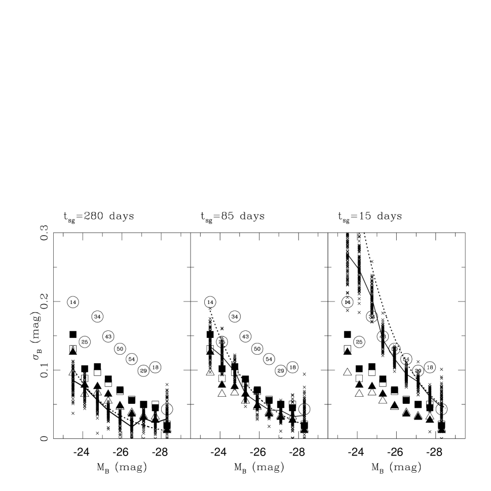
Figure 6: Variability–luminosity relationship found in the Monte Carlo simulations of the SGP sample, compared with the measured relationship for the data. Crosses represent the values found for 100 simulated samples, and the thick solid line represents the median value of the r.m.s. measured in those 100 simulated samples. The dashed line represents the theoretical approximation for variability derived in magnitudes in the low variability regime Open circles represent the r.m.s. of the observed QSOs in SGP. Open squares and triangles represent the same relationship for the the SGP QSOs after applying the variability–wavelength correction given by equation (18), such that a factor 2 in the $\sigma(\hbox{$\lambda$1350 \AA})/\sigma_{B}$ ratio is represented by squares and a factor 3 by triangles. Filled squares and triangles represent the rms of SGP QSOs after correcting the wavelength dependence of variability with a power–law of indices $-0.6$ and $-1.0$ respectively (factors 2 and 3 for the same ratio), as given by equation (19). The numbers enclosed by the open circles indicate the number of objects considered in the corresponding bin of luminosity to derive the variability indices: 14,25,34,43,50,54,29,18,4 from $M_{B}\approx-23.5$ to $-28.3$ mag.

The open circles in figure 6 represent the median of the r.m.s. $\sigma(\hbox{$M_{\mbox{\scriptsize B}}$})$ of the observed QSOs, calculated as with the simulations. The numbers enclosed in the open circles indicate the number of QSOs used in each luminosity bin. Open squares and triangles represent the derived B-band variability found after applying the linear variability–wavelength correction described by equation (21), where squares correspond to a factor 2 in the ratio $\sigma(\hbox{$\lambda$1350 \AA})/\hbox{$\sigma_{\mbox{\scriptsize B}}$}$, and triangles to a factor 3. Similarly, filled symbols represent the variability found in the data after applying the power-law correction given by equation (22), in order to reproduce factors 2 (squares) and 3 (triangles) in the ratio $\sigma(\hbox{$\lambda$1350 \AA})/\hbox{$\sigma_{\mbox{\scriptsize B}}$}$.

The agreement between models and data must be judged by the intersection of circles, triangles and squares with the bands of crosses, which show the range of $\sigma_{\mbox{\scriptsize B}}$ found for the 100 simulated data sets. The model which best reproduces the SGP data (circles), without any variability-wavelength correction, is that of fast intrinsic variations $\hbox{$t_{\mbox{\scriptsize sg}}$}=15$ days. Objects fainter than $-24$ mag can also be fit by a model with moderately fast intrinsic variations, between $\hbox{$t_{\mbox{\scriptsize sg}}$}=85$ days and $\hbox{$t_{\mbox{\scriptsize sg}}$}=15$ days. The model with Seyfert 1 like variations, $\hbox{$t_{\mbox{\scriptsize sg}}$}=280$ days, can definitely be ruled out at the luminosities of interest, except, maybe, for QSOs in the last bin ($\hbox{$M_{\mbox{\scriptsize B}}$}\approx-28.3$ mag), which, nevertheless, reach the error subtraction uncertainty limit. However, when a variability–wavelength correction is applied (squares and triangles), the data is best described in all luminosity bands by models with slow Seyfert 1 like variations ($\hbox{$t_{\mbox{\scriptsize sg}}$}=280$ days) or with moderate variations ($\hbox{$t_{\mbox{\scriptsize sg}}$}=85$ days), depending on the choice of variability–wavelength correction. Data corrected with $\sigma(\hbox{$\lambda$1350 \AA})/\hbox{$\sigma_{\mbox{\scriptsize B}}$}\approx 2$ laws (squares) are best described by moderate variations, while data corrected with $\sigma(\hbox{$\lambda$1350 \AA})/\hbox{$\sigma_{\mbox{\scriptsize B}}$}\approx 3$ laws (triangles) are equally well described by Seyfert 1 like and moderate variations. The fast variation models ($\hbox{$t_{\mbox{\scriptsize sg}}$}=15$ days) give a poor description of the variability–wavelength corrected data, except for the last two luminosity bins ($\hbox{$M_{\mbox{\scriptsize B}}$}\mathrel{\lower 2.5pt\vbox{\hbox{$<$}\hbox{$\sim$}}}-27.5$ mag).

3.4. Structure function

We also measure in the simulated samples the ensemble structure function, defined as

$$\hbox{$\mbox{SF}$}(\Delta t)=<\left({\hbox{$M_{\mbox{\scriptsize B}}$}_{i,k}-\hbox{$M_{\mbox{\scriptsize B}}$}_{i,l}}\right)^{2}>_{\mbox{\scriptsize median}}\mbox{\ \ \ ,}$$ (23)

where $k,l$ are all the combination of epochs of the $i$-th QSO that have a time interval $|t_{k}-t_{l}|$ comprised by $\Delta t$, and the median is calculated over the magnitude differences of all QSOs in the bin of interest. This ensemble structure function considers all the individual light curves of QSOs as a whole, since the poor sampling prevents the derivation of structure functions for individual sources.

The crosses in figure 7 represent the square root of the structure functions measured in the 100 simulated samples corresponding to each $t_{\mbox{\scriptsize sg}}$ value. The time bins for computing median values are set to be a year for pairs of epochs with $\Delta t>1$ yr, and half a year for pair of epochs with $\Delta t\leq 1$ yr, in order to map the rising of the structure function. The thick dashes in figure 7 mark the median values of the 100 realizations. The open circles represent the ensemble structure function measured in the data, where the number enclosed indicates the number of magnitude differences per bin. As above, squares and triangles represent the structure function of the data, once these are corrected for the variability-wavelength dependence with the parameterizations given by equations (21) (open symbols) and (22) (filled symbols), to reproduce factors of 2 (squares) or 3 (triangles) in the $\sigma(\hbox{$\lambda$1350 \AA})/\hbox{$\sigma_{\mbox{\scriptsize B}}$}$ ratio.

Figure 7: Square root of the structure function measured in the Monte Carlo simulations of the SGP sample, compared with the measured function of the observed sample. All the QSO light curves are treated as an ensemble light curve. Crosses represent the individual SFs obtained for 100 simulated samples and thick solid dashes represent the median values of all the simulated samples. Open circles represent the SF of the observed sample. Open squares and triangles represent the SF same after applying a linear variability–wavelength correction, such that a factor 2 in the $\sigma(\hbox{$\lambda$1350 \AA})/\sigma_{B}$ ratio is described by squares and a factor 3 by triangles. Filled squares and triangles represent the data after correcting the wavelength dependence of variability with a power–law of indices $-0.6$ and $-1.0$ respectively (factors 2 and 3 for the same ratio). The numbers enclosed by the open circles give the total number of differences involved in the derivation of the structure function for the corresponding bin of time: 1725,670,590,878,1170,1063,642 from $\Delta t\approx 0.5$ to 0.55 yr.

From the comparison of the intersection of crosses, squares, triangles and circles in figure 7, we deduce that the way in which the variability of the QSO sample is attained is well described by models involving $\hbox{$t_{\mbox{\scriptsize sg}}$}=85\mbox{\ to \ }280$ days, if one allows for a variability–wavelength correction as that observed in nearby AGN. If no variability–wavelength correction is applied, the data cannot be described by a single parameter model. Although the short variation models ($\hbox{$t_{\mbox{\scriptsize sg}}$}=15$ days) reproduce the final variability level of the data with no variability–wavelength correction, the first two time bins of the SF show that the growth curve of this model is quicker than that exhibited by the data. The quality of the data does not allow to probe the models to a higher degree. The most important difference among models with different $t_{\mbox{\scriptsize sg}}$ values is the time scale in which the flattening point of the SF is to appear. This flat regime is attained in time scales that the present data is unable to map in greater detail. In order to have a better description of the rise of the SF, one would need observations with time intervals of the order of, at least, months.

We must note that the ensemble SF defined by equation (23) combines QSO light curves with different variability amplitudes. Since QSOs of different amplitudes of variability, on average, correspond to different luminosities (figure 6), and those QSOs happen to be at different redshifts (figure 5), then, different time bins in the SF will be dominated by a different population of QSOs, i.e. those which happen to have pairs of observations with rest frame time intervals included in that particular time bin. If the mixture of QSOs changes from bin to bin, as is normally the case, the level of variability mapped for each bin in the ensemble SF will be dominated by differences in the degree of variability of different mixtures, and those variability differences will mask the genuine shape of the SF of individual QSOs. We can see that the scale invariant SF of figure 4 is not reproduced in the simulated samples (figure 7), just because the asymptotic value of the SF for each simulated QSO is different. Therefore, when the SFs of different data sets are compared, the ensemble SFs can easily differ just because the dominant population of QSOs in each bin has a different degree of variability due to (a) a different distribution of the QSOs in the luminosity–redshift plane or (b) a different observing sampling pattern. Differences in the SF of different data sets have already been reported by Cristiani and collaborators (1996). A normalized SF defined by

$$\hbox{$\mbox{SF}$}_{\mbox{\scriptsize n}}(\Delta t)\equiv<\left({\frac{\hbox{$M_{\mbox{\scriptsize B}}$}_{i,k}-\hbox{$M_{\mbox{\scriptsize B}}$}_{i,l}}{\sigma_{i}(\hbox{$M_{\mbox{\scriptsize B}}$})}}\right)^{2}>_{\mbox{\scriptsize median}}\mbox{\ \ \ ,}$$ (24)

where $\sigma_{i}(\hbox{$M_{\mbox{\scriptsize B}}$})$ is the r.m.s. of the light curve of the $i$-th QSO, would be a more powerful tool to establish differences in the intrinsic variability growth of different samples and populations of QSOs, getting rid, at the same time, of variability–wavelength dependences. From a theoretical point of view, the normalized SF is a more natural way of computing the ensemble SF, since the SFs of individual QSOs would be normalized to their asymptotic values, equation (19), before combining them. However, extracting the errors to the normalized SF is plagued with biases which arise in the distribution of normalized magnitude differences. This natural way of extracting information about the variability growth curve of QSOs will be investigated in a subsequent paper.

4. Discussion

4.1. QSOs as scaled up Seyfert 1 nuclei

We have shown that if high-redshift QSOs have a variability dependence with wavelength similar to that of nearby Seyfert nuclei and low-redshift ($z\mathrel{\lower 2.5pt\vbox{\hbox{$<$}\hbox{$\sim$}}}1$) QSOs, with $\sigma(\hbox{$\lambda$1350 \AA})/\hbox{$\sigma_{\mbox{\scriptsize B}}$}\sim 3$ ratios, their observed variability properties can be reproduced by a sequence of pulses with time-scales $\hbox{$t_{\mbox{\scriptsize sg}}$}\sim 280$ days. This value is also that found to reproduce the isolated long-term variations observed in the light curves of intensively monitored type 1 Seyfert nuclei (Aretxaga & Terlevich 1993,1994). Furthermore, the modelling we have performed in the previous sections adopts a linear proportionality between the number of individual pulses and the luminosity of the object (relation 2). These results imply that any model that considers QSOs as scaled versions of Seyfert nuclei can successfully reproduce the variability relationships found for radio-quiet AGN over a range of luminosities spanning, at least, 8 mag. In other words, our results show that the characteristics of the light curve of a QSO of $-27$ mag can be explained superposing the light curve of a Seyfert nucleus of $-21$ mag, like NGC 5548, about 250 times. The starburst model predicts such a behaviour through equation (2), and gives a natural explanation for the linear proportionality between the number of events and the global luminosity of the source: the link between the SN rate and the B band luminosity originated in the stars of the cluster (relation 1).

4.2. The masses of the stellar clusters and possible metallicity effects

In case the variability–wavelength relationship that applies to distant QSOs is flatter than a factor 3 in the $\sigma(\hbox{$\lambda$1350 \AA})/\hbox{$\sigma_{\mbox{\scriptsize B}}$}$ ratio, we have shown that the model requires shorter values for the intrinsic time of evolution of the postulated cSNRs in order to reproduce the variability–luminosity anti-correlation and the ensemble SF of QSOs. Values of $\sigma(\hbox{$\lambda$1350 \AA})/\hbox{$\sigma_{\mbox{\scriptsize B}}$}\approx 2\mbox{--}3$ would allow models with pulses of $\hbox{$t_{\mbox{\scriptsize sg}}$}\approx 85\mbox{--}280$ days to reproduce the observed variability relationships. Therefore, it is possible that the variability of distant QSOs is produced by shorter intrinsic variations than those observed in Seyfert 1 nuclei. In this subsection we would like to interpret such a possibility in the framework of the Starburst model.

The high SN rates required to explain high luminosity objects imply high masses for the stellar clusters. For typical QSOs with luminosities between $-24$ and $-27$ mag, the masses of the postulated coeval stellar clusters vary from $2\times 10^{10}$ to $3\times 10^{11}$ M_⊙, for a solar neighbourhood Initial Mass Function (see figure 3a of Aretxaga & Terlevich 1994). The mass estimation changes with the shape of the IMF and the age of the cluster. These values of the masses derived from the SN rates are well inside the hypothesis of Terlevich & Boyle (1993) that the QSO phenomenon might correspond to the formation of the cores of nowadays normal elliptical galaxies at $z\approx 2$. The most massive elliptical galaxies have masses of up to $10^{13}$ M_⊙ (Faber et al. 1989, Terlevich 1992). If that is the case, distant high luminosity QSOs are expected to have high metallicities, as high luminosity ellipticals do (Faber 1972,1973, Mould 1978). In fact, high metallicities of, perhaps, up to 10 Z_⊙ have been inferred from the emission line ratios of high luminosity QSOs (Hamann & Ferland 1993). The result of having a higher metallicity environment is translated into having shorter times of evolution for cSNRs. The reason is two fold, first one expects that stars would create a higher density circumstellar environment (Abbott, Bohlin & Savage 1982, Kudritzky, Pauldrach & Puls 1987) which is able to reprocess the kinetic energy into radiation more rapidly and, second, radiative cooling of the gas is more efficient at high metallicities, which also accelerates the evolution of the cSNR.

From the analysis of the SGP data set we cannot clearly isolate metallicity effects, i.e. variations of $t_{\mbox{\scriptsize sg}}$ with luminosity, although some variation might be reflected in the duality of the success of the models with $\hbox{$t_{\mbox{\scriptsize sg}}$}\sim 280\mbox{ -- }85$ days for the variability–wavelength corrected data and, certainly, in the comparison of these values with those derived for the light curves of Seyfert nuclei: 260–280 days (Aretxaga & Terlevich 1993,1994). If indeed there is any evolution in $t_{\mbox{\scriptsize sg}}$, the variability process will not be a simple Poissonian one, as explained in section 2.1

5. Conclusions

We have presented analytical predictions for the variability expected in a young stellar cluster with cSNR. We find that:

1. Luminous clusters are characterized by large SN rates, such that the amplitude of their variations is low due to the combined effect of the superposition of events and the dilution caused by the underlying stellar cluster light

2. The unit of variability (a SN$+$cSNR event) has an effective lifetime of a few years. The maximum degree of variability in a cluster is attained at the time when the variations produced by old SNe die out, i.e. when the baseline to measure the variability is larger than a few years. Therefore, variability versus time scale of variability relationships are expected to be flat at large baselines.

We have performed numerical simulations to compare the model predictions with the results obtained from the analysis of large data bases of QSOs. Our Monte Carlo simulations were parameterized to reproduce the time coverage and observational errors of one of the best QSO data bases available to date, the South Galactic Pole sample. The models we present have only one functional free parameter: the evolutionary time scale of the cSNRs in the stellar cluster ($t_{\mbox{\scriptsize sg}}$). Typical clusters with luminosities between $-24$ and $-27$ mag have a rate of SN explosions of 5–100 yr^-1. We have shown that the r.m.s. index and ensemble SF of the SGP sample can be reproduced with models in which the intrinsic variations are described by $t_{\mbox{\scriptsize sg}}$ values about 85–280  days, once a wavelength–variability correction typical of nearby AGN is applied to the sample of QSOs. The values of the $t_{\mbox{\scriptsize sg}}$ parameter obtained for type 1 Seyfert nuclei (Aretxaga & Terlevich 1993,1994) and observed cSNRs (Terlevich 1994) are also around 280 days. From these simulations we conclude that, if the wavelength–variability correction of QSOs is between the explored values of $\sigma(\hbox{$\lambda$1350 \AA})/\hbox{$\sigma_{\mbox{\scriptsize B}}$}\approx 2\mbox{--}3$, corresponding to those observed in low-redshift QSOs:

• The variability–luminosity anti–correlation measured in QSOs is consistent with that expected from a simple Poissonian process, and can be naturally explained by the multiple superposition of SN events. Given that previous work has shown that the light curves of Seyfert galaxies can be well modeled with a sequence of SN+cSNR events, we concluded that QSO variability can be regarded as a scaled up version of Seyfert variability.

• The shape of the SF is well matched by that predicted by SN$+$cSNR events. The flattening point in the structure functions of QSOs is the key signature of the characteristic evolutionary time scale of the postulated cSNRs. It is essential to concentrate the observational effort into mapping the rising of the SF in monthly time-scales. Such mapping is a powerful discriminator among different parameters for the models.

• The SN rates derived from QSO luminosities can reproduce the observed variability inside the restricted range of $t_{\mbox{\scriptsize sg}}$ values considered ( $85\leq\hbox{$t_{\mbox{\scriptsize sg}}$}\leq 280$ days ). The masses of the clusters derived from these rates, are in good agreement with those of the young cores of elliptical galaxies postulated by Terlevich & Boyle (1993) to model the luminosity function of QSOs.

• Although we cannot identify a clear trend of $t_{\mbox{\scriptsize sg}}$ values with luminosity, the data is consistent with some evolution in the characteristic lifetime of the postulated cSNRs, as expected from a higher metallicity environment at higher redshift. This would imply a simple Poissonian process for each QSO, but with different pulse characteristics for QSOs of different luminosities, so that the ensemble variability doen’t correspond to that of a simple Poissonian process any longer.

• The random superposition of individual variations in luminous systems creates smooth structures in the light curves with time scales of several years. These smooth variations are actually observed in moderately well sampled light curves of QSOs (Pica et al. 1988, Hawkins 1993, Maoz et al. 1994)

Clearly, a deeper study of these effects is needed through, possibly, the combination of large data bases as SGP, with similar or lower observational errors. Larger samples, a more complete covering of the luminosity–redshift plane and better sampling of the light curves would certainly allow a more stringent test of the models presented here.

More generally, we have shown that the wavelength dependence of variability must be taken into account when analyzing the variability properties of QSOs observed in a fixed band. However, the functional form of such a dependence is still empirically unknown and future work should concentrate on establishing an accurate wavelength–variability relationship from the UV to the optical. The forms used in this paper were just exploratory, taking into account the fact that nearby Seyfert nuclei and low-redshift QSOs exhibit a $\sigma(\hbox{$\lambda$1350 \AA})/\hbox{$\sigma_{\mbox{\scriptsize B}}$}\approx 2\mbox{--}3$. A detailed observational study on multi-wavelength variability of high-redshift objects should address the question of whether such an approximation is valid for high-redshift objects.

A final caveat is that in all our analysis we have disregarded the possible contribution to the emitted light by the underlying galaxy. At high redshifts this contribution may become important. Future work should explore this possible contribution.

References

- [1] Abbott D.C., Bohlin R.C., Savage B.D., 1982, ApJS, 48,369
- [2] Alloin D., Pelat D., Phillips M.M., Fosbury R., Freeman K., 1986, ApJ, 308,23
- [3] Aretxaga I., 1993, PhD thesis, Universidad Autónoma de Madrid
- [4] Aretxaga I., Terlevich R.J., 1993, ApSS, 206,69
- [5] Aretxaga I., Terlevich R.J., 1994, MNRAS, 269,462
- [6] Aretxaga I., Boyle B.J., Terlevich R.J., 1995, MNRAS, 275,L27
- [7] Bonoli F., Bracessi A., Federici L., Zitelli V., Formiggini L., 1979, A&AS, 35,391
- [8] Branch D., Falk S.W., McCall M.L., Rybski P., Uomoto A.K., Wills B.J., 1981, ApJ, 244,780
- [9] Cid Fernandes R., 1995, PhD thesis, Cambridge Univ. (available at http://www.if.ufrgs.br/cid)
- [10] Cid Fernandes R., Aretxaga I., Terlevich R.J., 1996, MNRAS, in press.
- [11] Cid Fernandes R., Terlevich R.J., Aretxaga I., 1996, MNRAS, submitted.
- [12] Clavel J. etal, 1987, ApJ, 321,251
- [13] Clavel J. etal, 1990, MNRAS, 246,668
- [14] Clavel J. etal, 1991, ApJ, 366,64
- [15] Cristiani S., Vio R., Andreani P., 1990, AJ, 100,56
- [16] Cristiani S., Trentini S., La Franca F., Aretxaga I., Andreani P., Vio R., 1996, A&A, 306,395
- [17] Edelson R., Krolik J., Pike G., 1990, ApJ, 359,86
- [18] Di Clemente A., Giallongo E., Natali G., Trevese D. & Vagneti F. 1996, preprint, to appear in Ap. J.
- [19] Faber S.M., 1972, A&A, 20,361
- [20] Faber S.M., 1973, ApJ, 179,731
- [21] Faber S.M., Wegner G., Burstein D., Davies R.L., Dressler A., Lynden-Bell D., Terlevich R., 1989, ApJS, 69,763
- [22] Filippenko A.V., 1989, AJ, 97,726
- [23] Franco J., Miller W.W.I., Arthur S.J., Tenorio-Tagle G., Terlevich R., 1994, ApJ, 435,805
- [24] Giallongo E., Trevese D., Vagnetti F., 1991, ApJ, 377,345
- [25] Hamann F., Ferland G., 1992, ApJ, 391,L53
- [26] Hamann F., Ferland G., 1993, ApJ, 418,11
- [27] Hawkins M.R.S., 1983, MNRAS, 202,571
- [28] Hawkins M.R.S., 1986, MNRAS, 219,417
- [29] Hawkins M.R.S., 1993, Nat, 366,242
- [30] Hook I.M., McMahon R.G., Boyle B.J., Irwin M.J., 1994, MNRAS, 268,305
- [31] Hutchings J., 1995, AJ, 110,994
- [32] Kinney A.L., Bohlin R.C., Blades J.C., York D.G., 1991, ApJS, 75,645
- [33] Kudritzky R.P., Pauldrach A., Puts J., 1987, A&A, 173,293
- [34] Maoz D., Smith P.S., Jannuzi B.T., Kaspi S., Netzer H., ApJ, 421, 34,.
- [35] McGimsey B.Q., Smith A.G., Scott R.L., Leacock R.J., Edwards P.L., Hackney K.L., Hackley K.R., 1975, AJ, 80,895
- [36] Mould, J., 1978, ApJ, 220,434
- [37] Osterbrock D.E., 1991, Rep. Prog. Phys, 54,579
- [38] Paltani S., Courvoisier T., 1994, A&A, 291,74
- [39] Peterson B.M. etal, 1991, ApJ, 368,119
- [40] Pica A.J., Smith A.G., 1983, ApJ, 272,11
- [41] Pica A.J., Smith A.G., Webb J.R., Leacock R.J., Clemens S. & Gombola P.P., 1988, AJ, 96,1215
- [42] Plewa T., 1995, MNRAS, 275,143
- [43] Searle L., Sargent W.L., 1968, ApJ, 153,1003
- [44] Scott R.L., Leacock R.J., McGimsey B.Q., Smith A.G., Edwards P.L., Hackney K.R., Hackney R.L., 1976, AJ, 81,7
- [45] Shuder J.M., 1981, ApJ, 244,12
- [46] Shull J.M., 1980, ApJ, 237,769
- [47] Simonetti J.H., Cordes J.M., Heeschen D.S., 1985, ApJ, 296,46
- [48] Smith A.G., Nair A.D., Leacock R.J., Clemens S.D., 1993, AJ, 105,437
- [49] Snijders M.A.J., 1991, in Duschl W.J., Wagner S.J., Camenzind I., eds, Variability of Active Galaxies. Springer-Verlag, Berlin, p. 9.
- [50] Stathakis R.A., Sadler E.M., 1991, MNRAS, 250,786
- [51] Tenorio-Tagle G., Terlevich R.J., Rozyczka M., Franco J. 1996, in preparation.
- [52] Terlevich R.J., 1992, in Filippenko A.V. eds, Relationships between Active Galactic Nuclei and Starburst Galaxies. A.S.P. Conference Proceedings, Vol. 31, p. 133.
- [53] Terlevich R.J., 1994, in Clegg R.E.S., Stevens I.R., Meikle W.P.S., eds, Circumstellar Media in the Late Stages of Stellar Evolution. Cambridge Univ. Press, Cambridge, p. 153
- [54] Terlevich R.J., Boyle B.J., 1993, MNRAS, 262,491
- [55] Terlevich R.J., Tenorio-Tagle G., Franco J., Melnick J., 1992, MNRAS, 255,713
- [56] Terlevich R.J., Tenorio-Tagle G., Franco J., Boyle B., Rozyczka M., Melnick J, 1993, in Rocca-Volmerange B. etal, eds., First Light in the Universe: Stars or QSO’s?. Editions Frontieres.
- [57] Terlevich R.J., Tenorio-Tagle G., Franco J., Rozyczka M., Melnick J., 1995, MNRAS, 272,198
- [58] Trevese D., Pitella G., Kron R.G., Koo D.C., Bershady M., 1989, AJ, 98,108
- [59] Trevese D., Kron, R.G., Majewski S.R., Bershady, M., Koo D.C., 1994, ApJ, 433,494
- [60] Turatto M., Cappellaro E., Danziger I.J., Benetti S., Gouiffes C., Della Valle M., 1993, MNRAS, 262,128
- [61] Wamsteker W. etal, 1990, ApJ, 354,446
- [62] Wheeler J.C., Mazurek T.J., Sivaramakrishnan A., 1980, ApJ, 237,781
- [63] Woosley S.E., 1988, in Kafatos N.M., Michalitsianos A., eds, Supernova 1987A in the Large Magellanic Cloud. Cambridge Univ. Press, Cambridge, p. 289
- [64] Yee H.K.C., 1980, ApJ, 241,894