Sensitivity of Galaxy Cluster Morphologies to $\Omega_{0}$ and $P(k)$

Abstract

We examine the sensitivity of the spatial morphologies of galaxy clusters to $\Omega_{0}$ and $P(k)$ using high-resolution N-body simulations with large dynamic range. Variants of the standard CDM model are considered having different spatial curvatures, SCDM $(\Omega_{0}=1)$, OCDM $(\Omega_{0}=0.35)$, LCDM $(\Omega_{0}=0.35,\lambda_{0}=0.65)$, and different normalizations, $\sigma_{8}$. We also explore critical density models with different spectral indices, $n$, of the scale-free power spectrum, $P(k)\propto k^{n}$. Cluster X-ray morphologies are quantified with power ratios (PRs), where we take for the X-ray emissivity $j_{gas}\propto\rho^{2}_{DM}$, which we argue is a suitable approximation for analysis of PRs. We find that $\Omega_{0}$ primarily influences the means of the PR distributions whereas the power spectrum ($n$ and $\sigma_{8}$) primarily affects their variances: $\log_{10}(P_{3}/P_{0})$ is the cleanest probe of $\Omega_{0}$ since its mean is very sensitive to $\Omega_{0}$ but very insensitive to $P(k)$. The PR means easily distinguish the SCDM and OCDM models, while the SCDM and LCDM means show a more modest, but significant, difference $(\sim 3\sigma)$. The OCDM and LCDM models are largely indistinguishable in terms of the PRs. Finally, we compared these models to a sample of $ROSAT$ clusters and find that the PR means of the SCDM clusters exceed the $ROSAT$ means with a high formal level of significance $(\sim 4\sigma)$. Though the formal significance level of this $\rho^{2}_{DM}$ / X-ray comparison should be considered only approximate, we argue that taking into account the hydrodynamics and cooling will not reconcile a discrepancy this large. The PR means of the OCDM clusters are consistent, and the means of the LCDM clusters are marginally consistent, with those of the $ROSAT$ clusters. Thus, we conclude that cluster morphologies strongly disfavor $\Omega_{0}=1$, CDM while favoring low density, CDM models with or without a cosmological constant.

1 Introduction

The quest for $\Omega_{0}$, the current ratio of the mean mass density of the universe to the critical density required for closure, has been a focus of the research efforts of many astrophysicists involving a variety of different techniques. At present, most observational evidence suggests a universe with sub-critical matter density, perhaps with a cosmological constant making up the difference required for a critical universe (e.g., Coles & Ellis 1994; Ostriker & Steinhardt 1995). The possibility of measuring $\Omega_{0}$ using the amount of “substructure” in galaxy clusters has thus generated some interest, “This is a critical area for further research, as it directly tests for $\Omega$ in dense lumps, so both observational and theoretical studies on a careful quantitative level would be well rewarded.” (Ostriker 1993).

Early analytical work (e.g., Richstone, Loeb, & Turner 1992) and simulations (Evrard et al. 1993; Mohr et al. 1995) found that the morphologies of X-ray clusters strongly favored $\Omega_{0}\sim 1$ over low-density universes. Along with $POTENT$ analysis of cosmic velocity fields (e.g., Dekel 1994), these substructure analyses were the only indicators in support of a critical value of $\Omega_{0}$. However, the analytical results (e.g., Kauffmann & White 1993; Nakamura, Hattori, & Mineshige 1995), simulations (e.g., Jing et al. 1994), and morphological statistics (e.g., Buote & Tsai 1995b) have been criticized rendering the previous conclusions about $\Omega_{0}$ uncertain.

Buote & Tsai (1995b, hereafter BTa) introduced the power ratios (PRs) for quantifying the spatial morphologies of clusters in terms of their dynamical states. The PRs essentially measure the square of the ratio of a higher order moment of the two-dimensional gravitational potential to the monopole term computed within a circular aperture, where the radius is specified by a metric scale (e.g., 1 Mpc). Buote & Tsai (1996, hereafter BTb) computed PRs of $ROSAT$ X-ray images for a sample of 59 clusters and discovered that the clusters are strongly correlated in PR space, obeying an “evolutionary track” which describes the dynamical evolution of the clusters (in projection). Tsai & Buote (1996, hereafter TB) studied the PRs of a small sample of clusters formed in the hydrodynamical simulation of Navarro, Frenk, & White (1995) and verified the interpretation of the “evolutionary track”. In contrast to the previous studies (e.g., Richstone et al. 1992; Mohr et al. 1995), TB concluded that their small cluster sample, formed in a standard $\Omega_{0}=1$, CDM simulation, possessed too much substructure (as quantified by the PRs) with respect to the $ROSAT$ clusters, and thus favored a lower value of $\Omega_{0}$.

However, a statistically large sample of clusters is important for studies of cluster morphologies. The PRs are most effective at categorizing clusters into different broad morphological types; i.e. the distinction between equal-sized bimodals and single-component clusters is more easily quantified than are small deviations in ellipticities and core radii between single-component clusters (see BTa). The efficiency of the PRs at classifying clusters into a broad range of morphological types is illustrated by their success at quantitatively discriminating the $ROSAT$ clusters along the lines of the morphological classes of Jones & Forman (1992) (see BTb). There is a lower frequency of nearly equal-sized bimodals in the $ROSAT$ sample than clusters with more regular morphologies. Hence, to make most effective use of the PRs the models need to be adequately sampled (i.e. simulations have enough clusters) to ensure that relatively rare regions of PR-space are sufficiently populated.

In this paper we build on the previous studies and investigate the ability of the PRs to distinguish between models having different values of $\Omega_{0}$. Unlike the previous theoretical studies of cluster morphologies mentioned above, we also consider models having different power spectra, $P(k)$, since $P(k)$ should affect the structures of clusters as well. At the time we began this project it was too computationally costly to use hydrodynamical simulations to generate for several cosmological models a large, statistically robust, number of clusters with sufficient resolution. To satisfy the above criteria and computational feasibility we instead used pure N-body simulations.

The organization of the paper is as follows. We discuss the selection of cosmological models in §2.1; the specifications of the N-body simulations in §2.2; the validity of using dark-matter-only simulations to generate X-ray images and the construction of the images in §2.3; and computation of the PRs in §2.4. We analyze the models having different values of $\Omega_{0}$ and a cosmological constant in §3, and models with different spectral slopes and $\sigma_{8}$ in §4. The implications of the results for all of the models and comparison of the simulations to the $ROSAT$ sample of BTb is discussed in §5. Finally, in §6 we present our conclusions.

2 Simulations

2.1 Cosmological Models

To test the sensitivity of cluster morphologies to the cosmological density parameter due to matter, $\Omega_{0}$, and the power spectrum of density fluctuations, $P(k)$, we examined several variants of the standard Cold Dark Matter (CDM) model (e.g., Ostriker 1993). In Table 1 we list the models and their relevant parameters: $\Omega_{0}$; $\lambda_{0}=\Lambda/3H^{2}_{0}$, where $\Lambda$ is a cosmological constant and $H_{0}$ is the present value of the Hubble parameter; the spectral index, $n$, of the scale-free power spectrum of density fluctuations, $P(k)\propto k^{n}$; and $\sigma_{8}$, the present rms density fluctuations in spheres of radius $8h^{-1}$ Mpc, where $h$ is defined by $H_{0}=100h$ km s^-1 Mpc^-1.

The parameters of the open CDM model (OCDM) and low-density, flat model (LCDM) were chosen to be consistent with current observations (e.g., Ostriker & Steinhardt 1995). Their normalizations were set according to the $\sigma_{8}-\Omega_{0}$ relationship of Eke, Cole, & Frenk (1996) to agree with the observed abundance of X-ray clusters. The biased CDM model (BCDM) was also normalized in this way. However, the BCDM simulation, because it has $\Omega_{0}=1$, necessarily has poorer resolution (i.e. fewer particles per cluster) than the OCDM and LCDM models due to the fixed box size of our simulations (see §2.3). For the purposes of our investigation of cluster morphologies it is paramount to compare simulations having similar resolution. Hence we use the SCDM model (with $\sigma_{8}=1$) as our primary $\Omega_{0}=1$ simulation for analysis, which has resolution equivalent to the OCDM and LCDM simulations. (We show in §4.4 that the means of the PR distributions for BCDM and SCDM are very similar which turns out to be most important for examining the effects of $\Omega_{0}$.) Hence, the SCDM, OCDM, and LCDM models allow us to explore the effects of $\Omega_{0}$ and $\lambda_{0}$ on the cluster morphologies; comparing SCDM and BCDM provides information on the influence of $\sigma_{8}$.

We explore the effects of different $P(k)$ on the PRs using the scale-free models, which have different $n$ from SCDM. For the scale-free models we normalized each to the same characteristic mass, $M_{\star}$, defined to be (Cole & Lacey 1996) the mass scale when the linear rms density fluctuation is equal to $\delta_{c}$, the critical density for a uniform spherically symmetric perturbation to collapse to a singularity. For $\Omega_{0}=1$, the linear theory predicts $\delta_{c}\approx 1.686$ (e.g., Padmanabhan 1993). We take the SCDM model with $\sigma_{8}=1$ as a reference for these scale-free models which gives a characteristic mass of $10^{14}M_{\sun}$. This procedure allows a consistent means to normalize the scale-free models relative to each other on the mass scales of clusters. Unfortunately, as a result of this normalization procedure, at earlier times the models have different large-scale power and thus the cluster mass functions are different for each of the models. The scale-free model with $n=-1.5$ is similar to the SCDM model and will be used to “calibrate” the scale-free models with respect to the other models (see Table 1).

2.2 N-body Cluster Sample

We use the Tree-Particle-Mesh (TPM) N-body code (Xu 1995b) to simulate the dissipationless formation of structure in a universe filled with cold dark matter. The simulations consist of $128^{3}$ particles in a square box of width $200h^{-1}$ Mpc. The gravitational softening length is $25h^{-1}$ kpc which translates to a nominal resolution of $\sim 50h^{-1}$ kpc. This resolution is sufficient for exploring the structure of clusters with PRs in apertures of radii $R_{ap}\gtrsim 0.5$ Mpc; for a discussion of the related effects of resolution on the performance of PRs on $ROSAT$ X-ray images see Buote & Tsai (1995b, §4). All of the realizations have the same initial random phase.

For each simulation we located the 39 most massive clusters using a version of the DENMAX algorithm (Bertschinger & Gelb 1991) modified by Xu (1995a). This convenient selection criterion yields well defined samples for each simulation and allows consistent statistical comparison between different simulations which is the principal goal of our present investigation. For the various cosmological models we explore (see Table 1) these clusters generally have masses ranging from $(0.3-3)\times h^{-1}10^{15}M_{\sun}$, which correspond to typical cluster masses observed in X-ray (e.g., Edge et al. 1990; David et. al. 1993) and optically (e.g., Carlberg et. al. 1995) selected samples.

2.3 X-ray Images

2.3.1 Motivation for $j_{g}\propto\rho^{2}_{DM}$

By letting the gas density trace the dark matter density $(\rho_{gas}\propto\rho_{DM})$ and by assuming that the plasma emissivity of the gas is constant, we computed the X-ray emissivity of the clusters, $j_{g}\propto\rho^{2}_{DM}$. Given its importance on the results presented in this paper, here we discuss at some length the suitability of this approximation. (Cooling of the gas is discussed in §5.1.)

For clusters in the process of formation or merging, the gas can have hot spots appearing where gas is being shock heated (e.g., Frenk, Evrard, Summers, & White 1996). One effect of such temperature fluctuations on the intrinsic X-ray emissivity is that the intrinsic plasma emissivity will vary substantially over the cluster thus rendering $j_{g}\propto\rho^{2}_{DM}$ a poor approximation. However, the intrinsic X-ray emissivity is not observed, but rather that which is convolved with the spectral response of the detector. For $ROSAT$ observations of clusters with the PSPC, the plasma emissivity is nearly constant over the relevant ranges of temperatures (NRA 91-OSSA-3, Appendix F, $ROSAT$ Mission Description), and thus temperature fluctuations contribute negligibly to variations in the emissivity; for previous discussions of this issue for the PRs see BTa and TB.

A more serious issue is whether the shocking gas invalidates the $\rho_{gas}\propto\rho_{DM}$ approximation, in which case the dynamical state inferred from the gas would not reflect that of the underlying mass. TB, who analyzed the hydrodynamical simulation of Navarro et al. (1995a), showed that the PRs computed for both the gas and the dark matter gave similar indications of the dynamical states of the simulated clusters (see §4 of TB). In particular, this applied at early times when the clusters underwent mergers with massive subclusters. Hence, our approximation for the X-ray emissivity should be reasonable even during the early, formative stages of clusters.

Another possible concern with setting $\rho_{gas}\propto\rho_{DM}$ is that a gas in hydrostatic equilibrium, which should be a more appropriate description for clusters in the later stages of their evolution, traces the shape of the potential of the gravitating matter which is necessarily rounder than the underlying mass; if the gas is rounder, then the PRs will be smaller. However, the core radius (or scale length) of the radial profile of the gas also influences the PRs. In fact, clusters with larger core radii have larger PRs; see BTa who computed PRs for toy X-ray cluster models having a variety of ellipticities and core radii.

When isothermal gas, which is a good approximation for a nearly relaxed cluster, is added to the potential generated by an average cluster formed in a $\Omega_{0}=1$, CDM simulation, the gas necessarily has a larger core radius than that of the dark matter (see Figure 14 of Navarro, Frenk, & White 1995b). Hence, a gas in hydrostatic equilibrium will have a larger core radius than that of the dark matter, at least in the context of the CDM models we are studying. Considering the competing effects of smaller ellipticity and larger core radii (factors of 2-3 in each), and from consulting Table 6 of BTa, we conclude that no clear bias in the PRs is to be expected by assuming that the gas follows the dark matter. In further support of this conclusion are the similarities of the morphologies of clusters in the N-body study of Jing et al. (1995). Using centroid-shifts and axial ratios they find similar results when $\rho_{gas}\propto\rho_{DM}$ and when the gas is in hydrostatic equilibrium (see their Figures 5, 6, and 8).

2.3.2 Construction of the Images

Having chosen our representation for the X-ray emissivity, we then generated two-dimensional “images” for each cluster. A rectangular box of dimensions $4\times 4\times 10$ $h^{-3}$ Mpc³ with random orientation was constructed about each cluster. We converted the particle distribution for each cluster to a mass density field using the interpolation technique employed in Smoothed Particle Hydrodynamics (SPH) (e.g., Hernquist & Katz 1989), from which the X-ray emissivity was generated, $j_{g}\propto\rho^{2}_{DM}$. The SPH interpolation calculates the density at a grid point by searching for the nearest neighbors and is thus more robust and physical than other linear interpolation schemes like Cloud-in-Cell. For our SPH interpolation we use 20 neighbors and the spline kernel described in Hernquist & Katz. The interpolation result is independent of the cell we choose for the X-ray emissivity calculations.

Typically, the boxes contained $\sim 2500$ particles for a cluster; e.g., SCDM (1799-3965), OCDM (1359-3656), LCDM (1439-3877), and BCDM (603-1740). We projected the emissivity along the long edge of the box into a square $4\times 4$ $h^{-2}$ Mpc² “image” consisting of “pixels” of width $20h^{-1}$ kpc. This pixel width was chosen sufficiently small so as not to inhibit reliable computation the PRs.

We do not add statistical noise or other effects associated with real observations to the X-ray images since our principal objective is to examine the intrinsic response of cluster morphologies to different cosmological parameters. However, the investigation of observational effects on the PRs by BTa, and the derived error bars on the PRs from $ROSAT$ clusters by BTb, do not show any large systematic biases; comparison of the simulations to the $ROSAT$ cluster sample is discussed in §5.

2.4 Power Ratios

The PRs are derived from the multipole expansion of the two-dimensional gravitational potential, $\Psi(R,\phi)$, generated by the mass density, $\Sigma(R,\phi)$, interior to $R$,

$$\Psi(R,\phi)=-2Ga_{0}\ln\left({1\over R}\right)-2G\sum^{\infty}_{m=1}{1\over mR^{m}}\left(a_{m}\cos m\phi+b_{m}\sin m\phi\right),$$ (1)

where $\phi$ is the azimuthal angle, $G$ is the gravitational constant and,

$$a_{m}(R) = \int_{R^{\prime}\leq R}\Sigma(\vec{x}^{\prime})\left(R^{\prime}\right)^{m}\cos m\phi^{\prime}d^{2}x^{\prime},$$ (2)

$$b_{m}(R) = \int_{R^{\prime}\leq R}\Sigma(\vec{x}^{\prime})\left(R^{\prime}\right)^{m}\sin m\phi^{\prime}d^{2}x^{\prime}.$$ (3)

Because of various advantageous properties of X-ray images of clusters, we associate the surface mass density, $\Sigma$, with X-ray surface brightness, $\Sigma_{X}$ (which is derived from the projection of $\rho^{2}_{DM}$ – see previous section); for more complete discussions of this association see BTa and TB. The square of each term on the right hand side of eq. (1) integrated over the boundary of a circular aperture of radius $R_{ap}$ is given by (ignoring factors of $2G$),

$$P_{m}={1\over 2m^{2}R^{2m}_{ap}}\left(a^{2}_{m}+b^{2}_{m}\right),$$ (4)

for $m>0$ and,

$$P_{0}=\left[a_{0}\ln\left(R_{ap}\right)\right]^{2},$$ (5)

for $m=0$. It is more useful for studies of cluster structure to consider the ratios of the higher order terms to the monopole term, $P_{m}/P_{0}$, which we call “power ratios” (PRs). By dividing each term by $P_{0}$ we normalize to the flux within $R_{ap}$. Because for clusters, $P_{m}/P_{0}\ll 1$ for $m>0$ (e.g., BTb), it is preferable to take the logarithm of the PRs,

$$PR_{m}\equiv\log_{10}{P_{m}\over P_{0}},$$ (6)

which we shall henceforward analyze in this paper.

Since the $P_{m}$ depend on the origin of the chosen coordinate system, we consider two choices for the origin. First, we take the aperture to lie at the centroid of $\Sigma_{X}$; i.e. where $P_{1}$ vanishes. Of these centroided $PR_{m}$, $PR_{2}$, $PR_{3}$, and $PR_{4}$ prove to be the most useful for studying cluster morphologies (see BTa). In order to extract information from the dipole term, we also consider the origin located at the peak of $\Sigma_{X}$. We denote this dipole ratio by $P^{(pk)}_{1}/P^{(pk)}_{0}$, and its logarithm $PR^{(pk)}_{1}$, to distinguish it from the centroided power ratios.

To obtain the centroid of $\Sigma_{X}$ in a consistent manner for all clusters we adopted the following procedure. First, when projecting the cluster (see §2.3), the cluster was roughly centered on the X-ray image by eye. For each image we computed the centroid in a circular aperture with $R_{ap}=1.5$ $h^{-1}$ Mpc located about the field center. This centroid was then used as our initial center for each cluster; see BTa for a description of how the peak of $\Sigma_{X}$ is located.

In addition to considering the $PR_{m}$ individually, we also analyze the cluster distributions along the “evolutionary tracks” in the $(PR_{2},PR_{4})$ and $(PR_{2},PR_{3})$ planes obeyed by the $ROSAT$ clusters of BTb. We refer the reader to TB for a detailed discussion of the cluster properties along the evolutionary tracks.

Using the augmented Edge et al. (1990) sample of BTb we recomputed the lines defining the evolutionary tracks of the $ROSAT$ data for the $1h^{-1}_{80}$ Mpc apertures. This was done since TB selected a subset of the clusters based on $PR_{m}$ measurement uncertainty rather than flux. Following TB we fit $PR_{4}=a+bPR_{2}$ considering the uncertainties in both axes ; a similar fit was done for the $(PR_{2},PR_{3})$ plane. We obtained $a=-0.92$, $b=1.18$ for the $(PR_{2},PR_{4})$ track which we denote by $PR_{2-4}$. Similarly, for the $(PR_{2},PR_{3})$ track, which we denote by $PR_{2-3}$, we obtained $a=-0.49$, $b=1.16$. These results are nearly the same found by TB for the slightly different sample.

To facilitate comparison to a previous study of the $PR_{m}$ of $ROSAT$ clusters (BTb), we compute $PR_{m}$ of the simulated clusters in apertures ranging in radius from $0.5h^{-1}_{80}$ Mpc to $1.5h^{-1}_{80}$ Mpc ($H_{0}=80h_{80}$ km s^-1 Mpc^-1) in steps of $0.25h^{-1}_{80}$ Mpc; i.e. $(0.4-1.2)h^{-1}$ Mpc in steps of $0.2h^{-1}$ Mpc. We refer the reader to §2 of BTa and §2 of TB for discussions of the advantages of using a series of fixed metric aperture sizes to study cluster morphologies.

3 $PR_{m}$ for Models with Different $\Omega_{0}$ and $\lambda_{0}$

First we consider clusters formed in the SCDM, OCDM, and LCDM models. Contour plots for 16 of the clusters formed in each of the models are displayed in Figures 1, 2, and 3. In Figure 4 we show the $(PR_{2},PR_{4})$ plane for the $0.5h^{-1}_{80}$ Mpc and $1.0h^{-1}_{80}$ Mpc apertures; the SCDM model appears in each plot for comparison. The clusters in each of the models exhibit tight correlations very similar to the evolutionary tracks of the $ROSAT$ clusters (BTb) and the simulated hydrodynamic clusters $(\Omega_{0}=1)$ of Navarro et al. (1995a) studied by TB. Along the evolutionary tracks a shift in the means of the $PR_{m}$ is easily noticeable in the $0.5h^{-1}_{80}$ Mpc aperture, being most apparent for the SCDM-OCDM models. The spread of the $PR_{m}$ along the track in the $1.0h^{-1}_{80}$ Mpc aperture for SCDM-OCDM also appears to be different. The distributions perpendicular to $PR_{2-4}$ do not show discrepancies obvious to the eye.

At this time we shift our focus away from the evolutionary tracks and instead analyze the individual $PR_{m}$ distributions, which prove to be more powerful for distinguishing between cosmological models as we show below. We give the individual $PR_{m}$ distributions of clusters in the three models for the $0.5h^{-1}_{80}$ Mpc and $1.0h^{-1}_{80}$ Mpc apertures in Figures 5 and 6. We found it most useful to compare these distributions in terms of their means, variances, and Kolmogorov-Smirnov (KS) statistics. For the number of clusters in each of our simulations (39) higher order statistics like the skewness and kurtosis are unreliable “high variance” distribution shape estimates (e.g., Bird & Beers 1993). We did consider more robust statistics like the “Asymmetry Index” (AI), which measures a quantity similar to the skewness, and the “Tail Index” (TI), which is similar to the Kurtosis (Bird & Beers 1993). However, we found that they did not clearly provide useful information in addition to the lower order statistics and KS test, and thus we do not discuss them further.

The means and standard deviations for the $(0.5,0.75,1.0)h^{-1}_{80}$ Mpc apertures are listed in Table 2. As a possible aid to understanding the relationships between the values in Table 7, we plot in Figure 7 the standard deviation vs the mean for the $0.75h^{-1}_{80}$ Mpc aperture. We do not present the results for the larger apertures because they did not significantly improve the ability to distinguish between the models. Moreover, we found that $PR_{4}$ and $PR^{(pk)}_{1}$ do not provide much useful information in addition to $PR_{2}$ and $PR_{3}$. Generally $PR_{4}$ tracks the behavior of $PR_{2}$, though showing less power to discriminate between models; the similarity to $PR_{2}$ is understandable given the strong correlation shown in Figure 4. Likewise, $PR^{(pk)}_{1}$ is similar to, but not quite so effective as, $PR_{3}$. For compactness, thus, we shall henceforward mostly restrict our discussion to results for $PR_{2}$ and $PR_{3}$ in the $(0.5,0.75,1.0)h^{-1}_{80}$ Mpc apertures.

We compare the means, standard deviations, and total distributions of the models in Table 3 using standard non-parametric tests as described in Press et al. (1994). The Student’s t-test, which compares the means of two distributions, computes a value, $p_{t}$, indicating the probability that the distributions have significantly different means. Similarly, the F-test, which compares the variances of two distributions, computes a value, $p_{F}$, indicating the probability that the distributions have significantly different variances. Finally, the KS test, which compares the overall shape of two distributions, computes a value, $p_{KS}$, indicating the probability that the distributions originate from the same parent population; the probabilities listed in Table 3 are given as percents; i.e. decimal probability times 100. Note that for the cases where the F-test gives a probability less than 5% we use the variant of the t-test appropriate for distributions with significantly different variances (i.e. program tutest in Press et. al.).

3.1 SCDM vs. OCDM

As is clear from inspection of Figures 4 - 7, and Tables 2 - 3, the means of the $PR_{m}$ of the SCDM model exceed those of OCDM. In terms of the t-test the significance of the differences is very high. Of all the $PR_{m}$, generally the means of $PR_{2}$ and $PR_{3}$ exhibit the largest significant differences; the most significant differences are seen for $PR_{3}$ in the $0.5h^{-1}_{80}$ Mpc aperture, $p_{t}=0.02\%$, and for $PR_{2}$ in the $0.75h^{-1}_{80}$ Mpc aperture, $p_{t}=0.06\%$. Hence, though different in all the apertures, the discrepancy in the means is most significant for the smallest apertures, $(0.5,0.75)h^{-1}_{80}$ Mpc.

The variances of $PR_{3}$ in the SCDM model are essentially consistent at all radii with their corresponding values in OCDM. However, for $PR_{2}$ the variances are consistent at $0.75h^{-1}_{80}$ Mpc, but marginally inconsistent at $(0.5,1.0)h^{-1}_{80}$ Mpc (and inconsistent at $(1.25,1.5)h^{-1}_{80}$ Mpc).

The KS test generally indicates a significant difference in SCDM and OCDM when also indicated by the t-test, or the t-test and F-test together. The level of discrepancy is usually not as significant as given by the t-test, except when $p_{F}$ is small as well. Since the KS test does not indicate discrepancy when both the t-test and F-test indicate similarity, we conclude that higher order properties of the PR distributions are probably not very important for the SCDM and OCDM models (at least for the samples of 39 clusters in our simulations). Since this qualitative behavior holds for the other model comparisons, we shall not emphasize the KS tests henceforward.

Finally, in terms of the various significance tests we find that the $PR_{2-4}$ distribution essentially gives a weighted probability of the individual $PR_{2}$ and $PR_{4}$ distributions; i.e. it does not enhance the discrepancy in the individual distributions. Perpendicular to $PR_{2-4}$ the distributions are consistent. The same behavior is seen for $PR_{2-3}$ as well. This behavior is seen for the remaining model comparisons in this section so we will not discuss the joint distributions further.

3.2 SCDM vs. LCDM

The $PR_{m}$ means for the SCDM clusters also systematically exceed those in the LCDM model, however the significance of the difference is not as large as with the OCDM clusters. The largest discrepancy is observed for $PR_{2}$ in the $(0.75,1.0)h^{-1}_{80}$ Mpc apertures for which $p_{t}=(0.7\%,0.8\%)$. The other $PR_{m}$ show only a marginal discrepancy in the means. For apertures $(0.5,0.75)h^{-1}_{80}$ Mpc, $PR_{3}$ has $p_{t}=(4\%,3\%)$, but is quite consistent at larger radii. The variances for the SCDM and LCDM models are consistent for essentially all radii and all $PR_{m}$.

3.3 OCDM vs. LCDM

The $PR_{m}$ means for the LCDM clusters appear to systematically exceed those in the OCDM model, however the formal significances of the differences are quite low. The means are entirely consistent at all radii for $PR_{2}$. However, $PR_{3}$ shows a marginal difference in the $0.5h^{-1}_{80}$ Mpc aperture ($p_{t}=9\%$). The variances of the $PR_{m}$ of the OCDM and LCDM models behave similarly as with the SCDM and OCDM comparison above, as expected since the SCDM-LCDM variances are essentially identical. However, the degree of discrepancy is not as pronounced.

3.4 Performance Evaluation I.

The means of the individual $PR_{m}$ distributions generally exhibit the most significant differences between the SCDM, OCDM, and LCDM models; the variances are much less sensitive to the models, with $PR_{3}$ showing no significant variance differences. The larger means for the $PR_{m}$ in the SCDM models are expected from the arguments of, e.g., Richstone et al. (1992). That is, in a sub-critical universe the growth of density fluctuations ceased at an early epoch and so present-day clusters should show less “substructure” than in an $\Omega_{0}=1$ universe where formation continues to the present. Clusters with more structure will have systematically larger values of the $PR_{m}$.

The $PR_{m}$ whose means show the most significant differences between the models are $PR_{2}$ and $PR_{3}$, where $PR_{2}$ typically performs best for apertures $(0.75,1.0)h^{-1}_{80}$ Mpc and $PR_{3}$ is most effective for $(0.5,0.75)h^{-1}_{80}$ Mpc. Although useful, $PR^{(pk)}_{1}$ is often the least effective $PR_{m}$ for differentiating models in terms of its mean; this relatively weak performance of the dipole ratio with respect to other moments is echoed in the results of Jing et al. (1995) who found that their measure of an axial ratio performed better than a centroid shift for discriminating between models (see their tables 3-6).

4 $PR_{m}$ for Models with Different $n$ and $\sigma_{8}$

In this section we investigate the effects of different power spectra for models otherwise conforming to the specifications of the SCDM model. First, we examine models with different spectral indices of the scale-free power spectrum $(P(k)\propto k^{n})$, $n=0,-1,-1.5,-2$. Then we examine the BCDM model which has a lower power-spectrum normalization as expressed by $\sigma_{8}$. As in the previous section, we find the $(0.5,0.75,1.0)h^{-1}_{80}$ Mpc apertures to be more useful than the larger apertures, and that $PR_{4}$ and $PR^{(pk)}_{1}$ do not provide much useful information in addition to that provided by $PR_{2}$ and $PR_{3}$. Hence, for compactness we again mostly restrict the discussion to $PR_{2}$ and $PR_{3}$ in the smaller apertures.

4.1 $n=-1.5$ vs. SCDM

Before analyzing the $PR_{m}$ of models with different $n$ we calibrate the scale-free models by comparing the $n=-1.5$ scale-free model to the SCDM model since they should have similar properties (see §2.1). We find that the means, variances, and KS statistics of the centroided $PR_{m}$ for the SCDM and $n=-1.5$ models are entirely consistent for all aperture radii with only one possible exception. The variances of $PR_{3}$ exhibit a marginal $(p_{F}=5\%)$ discrepancy in the $0.5h^{-1}_{80}$ Mpc aperture. The significance of this variance discrepancy should be treated with caution given the complete consistency of the means $(p_{t}=31\%)$ and KS (32%) test at this radius as well as the consistency of all the tests at all the other radii investigated. Hence, the cluster morphologies of the SCDM and $n=-1.5$ models are very consistent expressed in terms of the centroided $PR_{m}$ ($m=2,3,4$).

4.2 $n=0$ vs. $n=-2$

In Figure 8 we plot for the $n=0,-2$ models the PR correlations for $m=(2,3)$ and $m=(2,4)$ in the $(0.5,1.0)h^{-1}_{80}$ Mpc apertures. Histograms for the individual $PR_{m}$ in these apertures are displayed in Figures 9 and 10. Table 2 lists the means, Figure 11 plots the standard deviations versus the averages of the $PR_{m}$ in the $0.75h^{-1}_{80}$ Mpc aperture, and Table 3 gives the results of the significance tests.

The means of $PR_{3}$ are very consistent for the $n=0,-2$ models at all radii examined. Those for $PR_{2}$ may show some differences in their means, with the $n=-2$ models perhaps having systematically smaller values. The significance of the different means for $PR_{2}$ is only formally marginal, with $p_{t}=(11\%,4\%,10\%)\%$ for aperture radii $(0.5,0.75,1.0)h^{-1}_{80}$ Mpc.

However, the possible small differences in the means of $PR_{2}$ are dwarfed by the corresponding highly significant differences in its variances. Generally the variances for all the $PR_{m}$ in all the apertures are smaller for the $n=-2$ clusters. The most significant variance differences are observed for $PR_{2}$ which has $p_{F}<1\%$ in $(0.75,1.0)h^{-1}_{80}$ Mpc apertures and $p_{F}\sim 5\%$ for $0.5h^{-1}_{80}$ Mpc . The variances for $PR_{3}$ show differences but at a lower level of significance and only in the $(0.5,0.75,1.0)h^{-1}_{80}$ Mpc apertures; i.e. $p_{t}=(3\%,1\%,4\%)$.

Similar to what we found in §3, the differences implied by the KS test generally follow the significances implied by the t-test and F-test; i.e. higher order effects in the distributions are probably not overly important (at least for our sample sizes of 39 clusters). Moreover, again we find that analysis of the $PR_{m}$ in terms of the evolutionary tracks does not add useful information to the previous results. The mean and variance effects for the individual $PR_{m}$ translate to very similar behavior along $PR_{2-4}$. The direction perpendicular to $PR_{2-4}$ is essentially consistent for all of the tests. As a result, we do not emphasize the KS tests or the evolutionary tracks further.

4.3 Intermediate $n$

The behavior for other $n$ is similar, but depends to some extent on the range examined. We find that the range of $n$ which accentuates differences in the $PR_{m}$ is between $n=0,-1$. Over the range $n=0,-1$ the discrepancy of means for $PR_{2}$ essentially follows that of the full $n=0,-2$ discussed in §4.2. However, the variances are not so highly discrepant as before, with $p_{F}=3\%$ for $PR_{2}$ for aperture radii $(0.5,0.75)h^{-1}_{80}$ Mpc; elsewhere the variances of $PR_{2}$ are consistent between the $n=0,-1$ models. Over the $n=0,-1$ range $PR_{3}$ is consistent for all statistics at all radii examined.

The $PR_{m}$ exhibit very few differences over the range of indices $n=-1,-2$. For all radii examined the means and KS statistics are consistent for all the $PR_{m}$. However, the variances do show some marginal differences. The $1.0h^{-1}_{80}$ Mpc apertures has the most significance difference where $p_{F}=1.5\%$ for both $PR_{2}$ and $PR_{3}$. Also in the $0.75h^{-1}_{80}$ Mpc aperture $PR_{2}$ has $p_{F}=7\%$. Otherwise the variances of these $PR_{m}$ are consistent. (We mention that the variance of $PR_{2}$ for the $n=-1.5$ model in the $0.75h^{-1}_{80}$ Mpc aperture lies above that for the $n=-1$ model in Figure 11, but the difference is not statistically significant.)

4.4 SCDM vs. BCDM

Now we consider the $\Omega_{0}=1$, CDM model with a lower normalization, $\sigma_{8}=0.51$, which we refer to as the biased CDM model, BCDM. The means and variances for the BCDM model are listed in Table 2, the standard deviation versus the average $PR_{m}$ in the $0.75h^{-1}_{80}$ Mpc aperture are plotted in Figure 11, and the results for the significance tests in comparison to SCDM are given in Table 3.

The means of all the $PR_{m}$ at all aperture radii are consistent for the SCDM and BCDM models. The $PR_{m}$ variances of the SCDM clusters generally exceed those of the BCDM clusters. The significance levels of the differences are only marginal $(p_{F}\sim 3\%)$ and appear to be most important in the $0.75h^{-1}_{80}$ Mpc aperture.

It is possible that the slight variance differences between the SCDM and BCDM models are due to the difference in resolution between the two simulations; i.e. the clusters in the BCDM simulations contain about half the number of particles of the SCDM clusters. We would expect that the effects of resolution would be most important in the smallest apertures (which we do observe), although we would probably expect that the means as well as the variances would be affected (which we do not observe). We mention that the BCDM model performs virtually identically to the SCDM model when compared to the OCDM and LCDM models.

4.5 Performance Evaluation II.

The variances of the $PR_{m}$ show the most significant differences between models with different power spectra; $PR_{2}$ generally has the most sensitive variances over the parameter ranges explored. Decreasing $n$ and $\sigma_{8}$ both decrease the $PR_{m}$ variances, the differences being of similar magnitude for the $n=0,-1$ models and the SCDM and BCDM models. The means of the $PR_{m}$ are much less sensitive to the models with different $n$ and $\sigma_{8}$, with $PR_{2}$ showing the largest significant differences which are always less than differences in the variances. No significant differences in the means are observed for $PR_{3}$ over the range of power spectra studied.

The predominant effect of the power spectrum on the variances of the $PR_{m}$ is intriguing. It is reasonable that when the amount of small-scale structures is reduced (smaller $n$) or the population of cluster-sized structures is made more uniform (smaller $\sigma_{8}$) that the $PR_{m}$ distributions would also be more uniform. The observed low sensitivity of the $PR_{m}$ means to the power spectra is also reasonable since on average the $PR_{m}$ means should only be affected by the rate of mass accretion through the aperture of radius $R_{ap}$, not by the sizes of the individual accreting clumps.

5 Discussion

In the previous sections we have seen that differences in $\Omega_{0}$ and $P(k)$ in CDM models are reflected in the spatial morphologies of clusters when expressed in terms of the $PR_{m}$. For the purposes of probing $\Omega_{0}$, our analysis indicates that $PR_{3}$ is the best PR since its mean is quite sensitive to $\Omega_{0}$ but very insensitive to $P(k)$. It is advantageous to also consider $PR_{2}$ when a cosmological constant is introduced since its means differ for the SCDM and LCDM models by $\sim 3\sigma$ whereas $PR_{3}$ only distinguishes the models at the $\sim 2\sigma$ level. The marginal dependence of the mean of $PR_{2}$ on $P(k)$ is not overly serious for studying differences in $\Omega_{0}$ because the differences in means due to $P(k)$ are always accompanied by larger, more significant differences in the variances; i.e. different means for $PR_{2}$ but consistent variances should reflect differences only in $\Omega_{0}$. The best apertures for segregating models are generally $(0.5,0.75,1.0)h^{-1}_{80}$ Mpc.

A few previous studies have examined the influence of $\Omega_{0}$ and $\lambda_{0}$ on the morphologies of galaxy clusters. Perhaps the most thorough investigation is that of Jing et. al. (1995) who used N-body simulations of a variety of CDM models, including versions similar to our SCDM, OCDM, and LCDM, to study variations of center-shifts and axial ratios. Jing et. al. reached the same qualitative conclusions as we do; i.e. the SCDM model is easily distinguished from OCDM and LCDM because it produces clusters with much more irregular morphologies than than the others. However, Jing et al. obtained infinitesimal KS probabilities for the axial ratio when comparing SCDM to OCDM and LCDM, a level of significance orders of magnitude different from that found in this paper. The source of this discrepancy is unclear given the qualitative similarities of their axial ratio and our $PR_{2}$. The disagreement may arise from differences in numerical modeling between the simulations; i.e. the results of Jing et al. are derived from simulations with a larger force resolution ($0.1h^{-1}$ Mpc), and smaller particle number for the non-SCDM models ($64^{3}$) than in our simulations, and have clusters which visually do not show the rich structures seen in our simulations (Figures 1, 2, and 3).

The qualitative results of Jing et al. agree with the hydrodynamic simulations of Mohr et al. (1995) who also used center shifts and axial ratios as diagnostics for “substructure”. If we visually estimate the means of the center shifts and axial ratios from Figures 6 and 8 of Jing et al. for their SCDM, OCDM, and LCDM models (actually OCDM with $\Omega_{0}=0.2$ and LCDM with $\Omega_{0}=0.2,\lambda_{0}=0.8$), we find that they agree quite well with the corresponding values in Table 3 of Mohr et al.; i.e. the results from the N-body and hydrodynamic simulations are very similar, despite the many other differences between the simulations (e.g., large number of baryons in OCDM clusters for Mohr et al.).

We can make a similar comparison of the $PR_{m}$ derived in this paper with the results from TB who analyzed the small sample of SCDM clusters formed in the hydrodynamic simulation of Navarro et al. (1995a). We find that the means (and variances) of the $PR_{m}$ computed in this paper are very similar to those of the hydrodynamic clusters; e.g., the mean for $PR_{2-4}$ for $1h^{-1}_{80}$ Mpc may be read off Figure 7 of TB which shows excellent agreement with the SCDM value we obtain from the N-body simulations (average $PR_{2-4}=3.76$). The quantitative similarity between the results, particularly between the means of the morphological statistics, for the N-body and hydrodynamic simulations of (Jing et al.,Mohr et al.) and (this paper,TB) suggest that it is useful to compare the $PR_{m}$ derived from N-body simulations directly to the X-ray data.

5.1 Comparison to $ROSAT$ Clusters

Among the biases that need to be considered in such a comparison are the effects of cooling flows (e.g., Fabian 1994), selection, and noise. Cooling flows increase the X-ray emission in the cluster center, which has the effect on the $PR_{m}$ of essentially decreasing the core size of the cluster. Judging by the observed core radii of “regular” X-ray clusters we would expect at most a factor of $\sim 2$ difference in core radii (e.g., A401 vs. A2029 in Buote & Canizares 1996; also see Jones & Forman 1984). Changing the core radius by a factor of 2 typically changes $PR_{2}$ (for example) by a small fraction of a decade (see Table 6 of BTa); this behavior, as we show below, is confirmed using a more thorough treatment. The issue of biases between X-ray-selected and mass-selected samples needs to be addressed with hydrodynamical simulations. The estimated uncertainties of the $PR_{m}$ for the $ROSAT$ cluster sample of BTb, which take into account noise and unresolved sources, do not show any clear biases.

In Figure 12 we display the correlations of the centroided $PR_{m}$ for the $ROSAT$ sample of BTb in the $(0.5,1.0)h^{-1}_{80}$ Mpc apertures; the SCDM clusters are also plotted for a comparison. $PR_{m}$ histograms for these apertures are shown in Figure 13 and 14, along with those for the SCDM and OCDM models. We list the means and variances for the $ROSAT$ clusters in Table 4; we plot in Figure 15 the standard deviations versus the means for the $ROSAT$ clusters and models in the $0.5h^{-1}_{80}$ Mpc aperture; the results of the significance tests between the $ROSAT$ clusters and model clusters are given in Table 5. We analyze the $ROSAT$ clusters corresponding to the “updated Edge et. al. (1990)” flux-limited sample in BTb which gives 37 and 27 clusters respectively for the $(0.5,1.0)h^{-1}_{80}$ Mpc apertures; note that all the qualitative features of the results we obtain below are reproduced when all of the clusters studied in BTb are used (i.e. 59 and 44 clusters respectively).

The means of the SCDM clusters exceed those of the $ROSAT$ sample to a high level of significance, with the differences being most pronounced in the $0.5h^{-1}_{80}$ Mpc aperture. The most significant discrepancy is for $PR_{3}$ in the $0.5h^{-1}_{80}$ Mpc aperture for which $p_{t}=1.5\times 10^{-4}\%$. The variances for all the $PR_{m}$ except $PR_{3}$ are also significantly different, with the variances of the SCDM clusters exceeding those of the $ROSAT$ clusters. The SCDM model has $\sigma_{8}=1$ which is too high to fit other observations (e.g., Ostriker & Steinhardt 1995). The BCDM model, which has $\sigma_{8}=0.51$, does have $PR_{m}$ variances in better agreement with the $ROSAT$ sample. However, the means are in essentially the same level of disagreement. In fact, $PR_{2}$ has a much more significant mean discrepancy $(p_{t}=1.0\times 10^{-4}\%)$ in the $0.5h^{-1}_{80}$ Mpc aperture.

In contrast, the $PR_{m}$ have means that are entirely consistent for the OCDM and $ROSAT$ clusters in both apertures. The variances of the centroided $PR_{m}$ are significantly discrepant, particularly in the $1.0h^{-1}_{80}$ Mpc aperture, where the OCDM variances exceed the $ROSAT$ variances. This suggests a lower $\sigma_{8}$ or $n$ is needed to bring the variances of the OCDM models into agreement with the $ROSAT$ sample.

The $PR_{m}$ means of the LCDM clusters systematically exceed the $ROSAT$ means, but at a lower level of significance than does SCDM. The discrepancies are only significant in the $0.5h^{-1}_{80}$ Mpc aperture, where $PR_{3}$ $(p_{t}=0.4\%)$ and $PR^{(pk)}_{1}$ $(p_{t}=0.2\%)$ show the most significant discrepancies; the even $PR_{m}$ show at best a marginal discrepancy in their means $(p_{t}=10\%-15\%)$. The variances for the even $PR_{m}$ are also significantly different, though only in the $0.5h^{-1}_{80}$ Mpc aperture as well. As the LCDM and SCDM variances are very similar, we expect that the variance differences can be largely obviated with a lower value of $\sigma_{8}$.

The difference in the means of $PR_{3}$ for the LCDM and $ROSAT$ clusters in the $0.5h^{-1}_{80}$ Mpc aperture, though formally significant at better than the $3\sigma$ level, represents a shift of about one-half a decade in $PR_{3}$; also, when using all 59 clusters of BTb the significance is only $p_{t}=4\%$ ($\sim 2\sigma$). As we have discussed earlier, it is difficult to completely account for a discrepancy of this magnitude by invoking, e.g., the unsuitability of the $\rho_{gas}\propto\rho_{DM}$ approximation, observational noise, or cooling flows.

We may make a more precise estimate of the effects of cooling flows on the $PR_{m}$. The ROSAT clusters in the augmented Edge sample all have estimated mass-flow rates (Fabian 1994) from which we may compute a luminosity (bolometric) due to the cooling flow following Edge (1989), $L_{cool}=3.0\times 10^{41}h^{-2}_{50}\dot{M}T$ erg/s, where $\dot{M}$ is in $M_{\sun}$/year and $T$ is in keV. Comparing this cooling luminosity to the total cluster luminosity, $L_{bol}$, using the results of David et al. (1993) allows us to in effect remove the cooling gas from the ROSAT $PR_{m}$. To a first approximation the cooling flow affects only $P_{0}$ because the cooling emission is weighted heavily towards the aperture center. Hence, to approximately remove the effects of the cooling flows from the ROSAT clusters we reduce $P_{0}$ for each cluster by $(1-L_{cool}/L_{bol})$. We find that the $PR_{m}$ of the ROSAT clusters are modified minimally, the effect being that the means of the $PR_{m}$ are increased by $1/10$ of a decade: means for $PR_{2}$ and $PR_{3}$ are -5.60 and -7.52 respectively in the $0.5h^{-1}_{80}$ aperture; the variances show no significant systematic effect. These small mean shifts do reduce the significance of the LCDM-ROSAT discrepancy, but the discrepancy is still significant at the $\sim 3\sigma$ level; e.g., $p_{t}=1.6\%$ for $PR_{3}$ and $p_{t}=1\%$ for $PR^{(pk)}_{1}$ in the $0.5h^{-1}_{80}$ aperture, and $p_{t}=34\%$ for the even $PR_{m}$.

Although cooling flows alone cannot completely account for the differences in the ROSAT clusters and the LCDM model, it is very possible that when combined with the the other effects mentioned above a sizeable fraction of the half-decade difference could be made up which would in any event reduce the significance level of the difference. As a result, we believe the discrepancy of the LCDM-$ROSAT$ means must be considered preliminary and await confirmation from appropriate hydrodynamical simulations.

On the other hand, the means of $PR_{3}$ for the SCDM and BCDM models exceed the $ROSAT$ means by almost a full decade to a higher formal significance level $(\sim 4\sigma)$, which in light of the previous discussion should be considered robust. We conclude that the $\Omega_{0}=1$, CDM models cannot produce the observed $PR_{m}$ of the $ROSAT$ clusters, and that the discrepancy in $PR_{m}$ means is due to $\Omega_{0}$ being too large. This agrees with our conclusions obtained in TB for the small sample of clusters drawn from the hydrodynamic simulation of Navarro et al. (1995a).

Our conclusions are opposite those of Mohr et al. (1995) who instead concluded that their Einstein cluster sample favored SCDM over both OCDM and LCDM. Given the qualitative agreement discussed above between the Jing et al. and Mohr et al. simulations, as well as between our present simulations and TB, it would seem that the discrepancy lies not in the details of the individual simulations. Moreover, since the centroid shift is qualitatively similar to our $P^{(pk)}_{1}/P^{(pk)}_{0}$, and the axial ratio is qualitatively related to our $P_{2}/P_{0}$, it would seem unlikely that we would reach entirely opposite conclusions.

The other plausible variable is to consider how BTb and Mohr et al. computed their statistics on the real cluster data. The $ROSAT$ data analyzed by BTb have better spatial resolution and sensitivity than the Einstein data analyzed by Mohr et al.. This implies that the Mohr et al. data should be biased in the direction of less “substructure” with respect to BTb, which is the opposite of what is found. Another important difference between the two investigations is that the $PR_{m}$ are computed within apertures of fixed metric size, whereas Mohr et. al. use a $S/N$ criterion to define the aperture size. The fixed metric radius used by the $PR_{m}$ ensures that cluster structure on the scale $\sim R_{ap}$ is compared consistently which is not true for the $S/N$ criterion (see BTa); e.g., Mohr et al. use aperture sizes of $0.38h^{-1}_{80}$ Mpc for Coma and of $0.81h^{-1}_{80}$ Mpc for A2256. It is not obvious, however, how this confusion of cluster scales would explain the discrepancy of our results with Mohr et al..

6 Conclusions

Using the power ratios ($PR_{m}=\log_{10}(P_{m}/P_{0})$) of Buote & Tsai (1995 – BTa; 1996 – BTb; Tsai & Buote 1996 – TB) we have examined the sensitivity of galaxy cluster morphologies to $\Omega_{0}$ and $P(k)$ using large, high-resolution N-body simulations. X-ray images are generated from the dark matter by letting the gas density trace the dark matter. We argue that the $PR_{m}$ should not be seriously biased by this approximation because a real gas in hydrostatic equilibrium with potentials of CDM clusters is rounder, but also has a larger core radius, the effects of which partially cancel. We also argue that the approximation should be reasonable during mergers because of the agreement shown between the evolution of the dark matter and gas found by TB who analyzed the hydrodynamical simulation of Navarro et al. (1995a). Finally, The $PR_{m}$ generated from the N-body simulations in this paper agree with results from the Navarro et al. hydrodynamical simulation (TB). Similar agreement is seen between the results of the N-body simulations of Jing et al. (1995) and the hydrodynamical simulations of Mohr et al. (1995).

From analysis of several variants of the standard Cold Dark Matter model, we have shown that the $PR_{m}$ can distinguish between models with different $\Omega_{0}$ and $P(k)$. Generally, $\Omega_{0}$ influences the means of the $PR_{m}$ distributions such that larger values of $\Omega_{0}$ primarily imply larger average PR values. The slope of the power spectrum and $\sigma_{8}$ primarily influence the variances of the $PR_{m}$; smaller $n$ and $\sigma_{8}$ generally imply smaller $PR_{m}$ variances.

For examining $\Omega_{0}$, our analysis indicates that $PR_{3}$ is the best $PR_{m}$ since its mean is quite sensitive to $\Omega_{0}$ but very insensitive to $P(k)$. It is advantageous also to consider $PR_{2}$ when a cosmological constant is introduced since its means differ for the SCDM and LCDM models by $\sim 3\sigma$ whereas $PR_{3}$ only distinguishes the models at the $\sim 2\sigma$ level. The dependence of the mean of $PR_{2}$ on $P(k)$ is not overly serious for studying differences in $\Omega_{0}$ because the differences in means due to $P(k)$ are always accompanied by larger differences in the variances; i.e. different means but consistent variances mostly reflect differences in $\Omega_{0}$ for $PR_{2}$. Typically, the best apertures for segregating models are $(0.5,0.75,1.0)h^{-1}_{80}$ Mpc.

We did not find it advantageous to compare the distributions along and perpendicular to the “evolutionary tracks” in the $(PR_{2},PR_{4})$ and $(PR_{2},PR_{3})$ planes (see BTb and TB). The distributions along the tracks performed essentially as a weighted sum of the constituent $PR_{m}$. The distributions perpendicular to the tracks were in almost all cases consistent for the models. Hence, although the evolutionary tracks are useful for categorizing the dynamical states of clusters, they do not allow more interesting constraints on $\Omega_{0}$ and $P(k)$ to be obtained over the individual $PR_{m}$. The consistency of the distributions perpendicular to the evolutionary tracks seems to be a generic feature of the CDM models.

We compared the $PR_{m}$ of the CDM models to the $ROSAT$ cluster sample of Buote & Tsai (1996). We find that the means of the $\Omega_{0}=0.35$ OCDM and $ROSAT$ clusters are consistent, but the means of $PR_{3}$ for the LCDM and $ROSAT$ clusters are formally inconsistent at the $\sim 3\sigma$ level. We assert that this discrepancy should be considered marginal due to various issues associated with the simulation – observation comparison.

However, the means of $PR_{3}$ for the SCDM and BCDM models (with $\Omega_{0}=1$) exceed the $ROSAT$ means by almost a full decade with a high level of significance $(\sim 4\sigma)$. Though the formal significance level of this $\rho^{2}_{DM}$ / X-ray comparison should be considered only an approximation, we argue that taking into account the hydrodynamics and cooling will not reconcile a discrepancy this large. We conclude that the $\Omega_{0}=1$ CDM models cannot produce the observed $PR_{m}$ of the $ROSAT$ clusters, and that the discrepancy in $PR_{m}$ means is due to $\Omega_{0}$ being too large. This agrees with our conclusions obtained in TB for the small sample of clusters drawn from the hydrodynamic simulation of Navarro et al. (1995a). These conclusions are also consistent with other indicators of a low value of $\Omega_{0}$ such as the dynamical analyses of clusters (e.g., Carlberg et al. 1995), the large baryon fractions in clusters (e.g., White et al. 1993), and the heating of galactic disks (Toth & Ostriker 1992).

Our conclusions are inconsistent with those of Mohr et al. (1995) who instead concluded that their Einstein cluster sample favored $\Omega_{0}=1$, CDM over equivalents of our low-density models, OCDM and LCDM. We argue that this type of discrepancy is unlikely due to numerical differences between our simulations. We discuss possible differences due to how BTb and Mohr et. al. computed their statistics on the real cluster data.

Large hydrodynamical simulations are necessary to render the comparison to the $ROSAT$ data more robust. In addition, the effects of combining data at different redshifts needs to be explored since cluster formation rates should behave differently as a function of $z$ in different models (e.g., Richstone et. al. 1992). It may also prove useful to apply $PR_{m}$ to mass maps of clusters obtained from weak lensing (Kaiser & Squires 1993), though for cosmological purposes it is not clear whether $\rho_{mass}$ will be as responsive as $\rho^{2}_{gas}$ to different $\Omega_{0}$ and $P(k)$.

Table 1: Cosmological Models

Name	$\Omega_{0}$	$\lambda_{0}$	$n$	$\sigma_{8}$	$h$	$z_{i}$
SCDM	1	0	1	1.00	0.5	20
OCDM	0.35	0	1	0.79	0.7	25
LCDM	0.35	0.65	1	0.83	0.7	39
BCDM	1	0	1	0.51	0.5	20
SF00	1	0	0	$\ldots$	$\ldots$	$\ldots$
SF10	1	0	-1.0	$\ldots$	$\ldots$	$\ldots$
SF15	1	0	-1.5	$\ldots$	$\ldots$	$\ldots$
SF20	1	0	-2.0	$\ldots$	$\ldots$	$\ldots$

Table 2: Average Power Ratios

	$PR_{2}$						$PR_{3}$
	0.5 Mpc		0.75 Mpc		1.0 Mpc		0.5 Mpc		0.75 Mpc		1.0 Mpc
	avg	$\sigma$	avg	$\sigma$	avg	$\sigma$	avg	$\sigma$	avg	$\sigma$	avg	$\sigma$
SCDM	-5.14	0.86	-5.16	0.83	-5.38	0.76	-6.72	0.73	-6.82	1.01	-7.06	0.98
OCDM	-5.55	0.61	-5.82	0.78	-5.93	1.03	-7.40	0.81	-7.56	1.13	-7.59	1.28
LCDM	-5.45	0.83	-5.69	0.85	-5.87	0.83	-7.08	0.83	-7.32	1.00	-7.38	1.02
BCDM	-5.01	0.57	-5.24	0.60	-5.41	0.63	-6.83	0.65	-6.98	0.67	-7.07	0.68
SF00	-5.34	0.82	-5.64	1.00	-5.75	0.97	-7.12	1.02	-7.28	1.14	-7.35	1.10
SF10	-5.02	0.57	-5.22	0.71	-5.47	0.85	-6.89	0.87	-7.09	1.02	-7.36	1.18
SF15	-5.20	0.85	-5.22	0.94	-5.40	0.91	-6.92	0.99	-6.93	1.02	-7.05	0.96
SF20	-5.07	0.60	-5.24	0.62	-5.45	0.57	-7.01	0.71	-7.13	0.75	-7.20	0.79

Table 3: Significance Tests for Power Ratios

			0.5 Mpc			0.75 Mpc			1.0 Mpc
			$p_{t}$	$p_{F}$	$p_{KS}$	$p_{t}$	$p_{F}$	$p_{KS}$	$p_{t}$	$p_{F}$	$p_{KS}$
Models			(%)	(%)	(%)	(%)	(%)	(%)	(%)	(%)	(%)
$PR_{2}$
SCDM	vs.	OCDM	1.63	4.09	0.94	0.06	71.71	0.07	0.89	7.18	0.94
SCDM	vs.	LCDM	10.47	87.90	21.79	0.74	89.05	1.97	0.83	58.78	3.90
OCDM	vs.	LCDM	54.64	5.79	51.42	47.52	61.72	21.79	78.26	20.53	34.56
SCDM	vs.	BCDM	43.06	1.51	98.09	65.19	4.65	21.79	83.52	24.87	34.56
SF00	vs.	SF20	10.76	6.35	7.31	4.19	0.38	0.94	10.44	0.13	3.90
$PR_{3}$
SCDM	vs.	OCDM	0.02	52.99	0.18	0.31	46.71	0.94	4.43	10.64	7.31
SCDM	vs.	LCDM	4.44	43.91	21.79	3.26	97.10	7.31	15.88	81.58	51.42
OCDM	vs.	LCDM	9.10	88.39	21.79	30.99	44.52	51.42	43.51	16.61	51.42
SCDM	vs.	BCDM	49.58	47.26	70.85	40.62	1.39	34.56	97.46	2.48	70.85
SF00	vs.	SF20	57.65	2.89	21.79	49.89	1.28	21.79	50.92	4.31	12.97

Table 4: PR Statistics for $ROSAT$ Clusters

	0.5 Mpc		1.0 Mpc
	avg	$\sigma$	avg	$\sigma$
$PR_{2}$	-5.70	0.44	-6.00	0.50
$PR_{3}$	-7.62	0.77	-7.61	0.77

Table 5: Significance Tests for $ROSAT$ Clusters

	0.5 Mpc			1.0 Mpc
Models	$p_{t}(\%)$	$p_{F}(\%)$	$p_{KS}(\%)$	$p_{t}(\%)$	$p_{F}(\%)$	$p_{KS}(\%)$
$PR_{2}$
SCDM	0.60E-01	0.12E-01	0.68E-03	0.14E-01	0.24E+01	0.33E-01
BCDM	0.10E-04	0.12E+02	0.56E-04	0.12E-01	0.20E+02	0.12E-01
OCDM	0.23E+02	0.52E+01	0.16E+02	0.68E+02	0.23E-01	0.43E+02
LCDM	0.11E+02	0.21E-01	0.13E+01	0.41E+02	0.69E+00	0.23E+02
$PR_{3}$
SCDM	0.15E-03	0.71E+02	0.69E-01	0.17E+01	0.20E+02	0.10E+02
BCDM	0.64E-03	0.28E+02	0.32E-02	0.35E+00	0.46E+02	0.12E+02
OCDM	0.22E+02	0.80E+02	0.42E+02	0.93E+02	0.83E+00	0.29E+02
LCDM	0.44E+00	0.69E+02	0.97E+00	0.33E+02	0.14E+02	0.32E+02

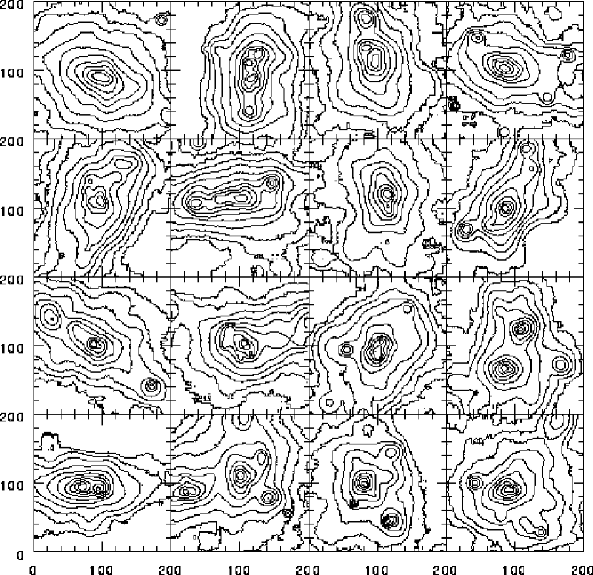
Figure 1:

Contour plots of the “X-ray Images” for 16 of the 39 clusters analyzed in the SCDM model obtained from projecting $j_{gas}\propto\rho^{2}_{DM}$. Each image is $4\times 4$ $h^{-2}$ Mpc² and the axes units are $20h^{-1}$ Mpc pixels.

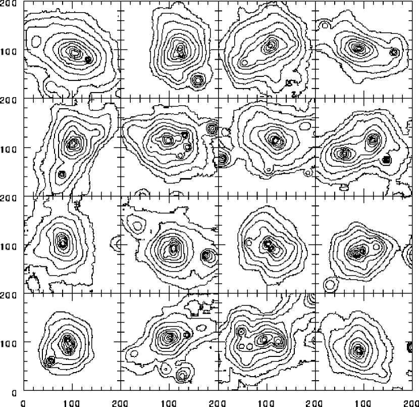
Figure 2:

As Figure 1, but for OCDM.

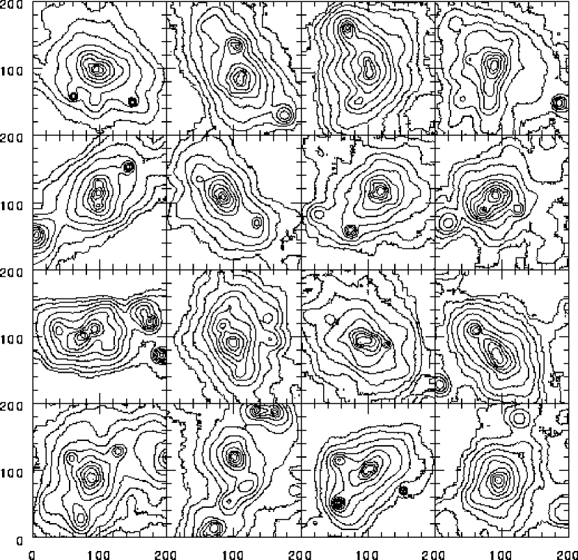
Figure 3:

As Figure 1, but for LCDM.

Figure 4:

Joint $PR_{m}$ distributions in the $(0.5,1.0)h^{-1}_{80}$ Mpc apertures for the SCDM, OCDM, LCDM, and BCDM models.

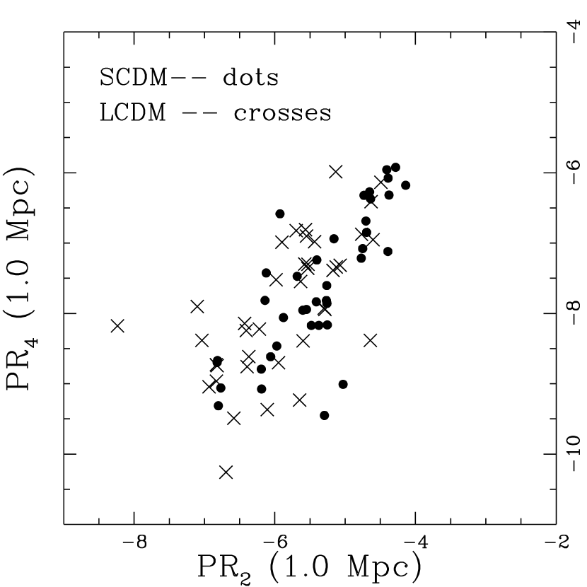
Figure 5:

Histograms for the PRs in the $0.5h^{-1}_{80}$ Mpc aperture. SCDM is given by the solid line, OCDM by the dotted line, and LCDM by the dashed line.

Figure 6:

As Figure 5, but for the $1.0h^{-1}_{80}$ Mpc aperture.

Figure 7:

The standard deviation as a function of the average value of the PRs in the $0.75h^{-1}_{80}$ Mpc aperture for the models in §3. The error bars represent $1\sigma$ errors estimated from 1000 bootstrap resamplings.

Figure 8:

Joint $PR_{m}$ distributions in the $(0.5,1.0)h^{-1}_{80}$ Mpc apertures for the scale-free models: SF00 $(n=0)$ denoted by dots and SF20 $(-2)$ denoted by crosses.

Figure 9:

Histograms for the $PR_{m}$ in the $0.5h^{-1}_{80}$ Mpc aperture. Spectral index $n=0$ (SF00) is given by the solid line and spectral index $n=-2$ (SF20) by the dotted line.

Figure 10:

As Figure 9, but for the $1.0h^{-1}_{80}$ Mpc aperture.

Figure 11:

The standard deviation as a function of the average value of the PRs in the $0.75h^{-1}_{80}$ Mpc aperture for the models in §4. The error bars represent $1\sigma$ errors estimated from 1000 bootstrap resamplings.

Figure 12:

Joint $PR_{m}$ distributions in the $(0.5,1.0)h^{-1}_{80}$ Mpc apertures for the $ROSAT$ (crosses) and SCDM (dots) clusters.

Figure 13:

Histograms for the PRs in the $0.5h^{-1}_{80}$ Mpc aperture. $ROSAT$ is given by the solid line, SCDM by the dotted line, and OCDM by the dashed line.

Figure 14:

As Figure 13, but for the $1.0h^{-1}_{80}$ Mpc aperture.

Figure 15:

The standard deviation as a function of the average value of the PRs in the $0.5h^{-1}_{80}$ Mpc aperture for the ROSAT clusters and the models discussed in §5.1. The error bars represent $1\sigma$ errors estimated from 1000 bootstrap resamplings.