SPECTRA OF UNSTEADY WIND MODELS
OF GAMMA-RAY BURSTS

Abstract

We calculate the spectra expected from unsteady relativistic wind models of gamma-ray bursts, suitable for events of arbitrary duration. The spectral energy distribution of the burst is calculated over photon energies spanning from eV to TeV, for a range of event durations and variability timescales. The relative strength of the emission at different wavelengths can provide valuable information on the particle acceleration, radiation mechanisms and the possible types of models.

1 Introduction

Relativistic wind models of Gamma Ray Bursts (GRB) are a recent development of the dissipative relativistic fireball scenario which is a natural consequence of observationally set requirements irrespective of the GRB distance scale (e.g. Mészáros (1995)). The observed bursts are expected to be produced in optically thin shocks in the later stages of the fireball expansion. Two types of shocks have been considered, based on different interpretations of the burst duration and variability. First, the “external” deceleration shocks (Rees & Mészáros (1992); Mészáros & Rees (1993)) that develop at $r_{dec}$, due to the unavoidable interaction of the relativistic ejecta with the surrounding medium, give bursts whose duration is determined (in the “impulsive” regime) by the relativistic dynamic timescale $t_{dec}\sim r_{dec}/c\Gamma^{2}$, where $\Gamma$ is the Lorentz factor of the expansion (e.g. Mészáros & Rees (1993); Katz (1994); Sari, Narayan & Piran 1996). Second, the “internal” dissipation shocks in an unsteady relativistic wind outflow (Rees & Mészáros (1994) [RM94]; Paczyński & Xu (1994)), where both the burst duration $t_{w}$ and time variability $t_{var}\leq t_{w}$, are characteristic of the progenitor mechanism (e.g. a disrupted disk accretion timescale, dynamic or turbulent timescales, etc.). Simple “external” shocks tend to produce fairly smooth light curves with a fast rise followed by an exponential decay (FRED), as observed in some bursts. However, many bursts have multi-peaked, irregular light curves; those may find a more natural explanation (Fenimore, Madras & Nayakshin 1996) in the relativistic wind scenario mentioned above.

While the spectral properties of impulsive “external” shocks have been studied in some detail (Mészáros, Rees & Papathanassiou (1994) [MRP94]; Sari et al. (1996)), so far, only rough estimates have been made for wind “internal” shock spectra (Mészáros & Rees (1994); Thompson (1994)). It is of great interest to explore the spectral properties of both types of shock scenarios, particularly in view of the increasingly sophisticated analyses of both GRB light curves (e.g. Fenimore et al. (1996); Norris et al. (1996)) and spectral characteristics (e.g. Band et al. (1993)). In this letter, we investigate the spectral properties of “internal” shocks for representative parameter values and discuss those properties in the light of anticipated results from HETE.

2 Physical Model and Shock Parameters

In the unsteady relativistic wind model, the GRB event is caused by the release of an amount of energy $E=10^{51}E_{51}$ erg, inside a volume of typical dimension $r_{\ell}=3\times 10^{10}t_{var}$ cm, over a timescale $t_{w}$ (RM94). The average dimensionless entropy per particle $\eta=\langle E/(Mc^{2})\rangle-1=\langle L/({\dot{M}}c^{2})\rangle$ determines the character of the overall flow. The bulk Lorentz factor of the flow increases as $\Gamma\propto r$ at first and later saturates to a value $\Gamma=\Gamma_{s}$ at $r\mathrel{\mathchoice{\lower 0.5pt\vbox{\halign{$\mathnew\displaystyle\hfil#\hfil$\cr>\crcr\sim\crcr}}}{\lower 0.5pt\vbox{\halign{$\mathnew\textstyle\hfil#\hfil$\cr>\crcr\sim\crcr}}}{\lower 0.5pt\vbox{\halign{$\mathnew\scriptstyle\hfil#\hfil$\cr>\crcr\sim\crcr}}}{\lower 0.5pt\vbox{\halign{$\mathnew\scriptscriptstyle\hfil#\hfil$\cr>\crcr\sim\crcr}}}}r_{s}\approx r_{\ell}\Gamma_{s}$, where $\Gamma_{s}\sim\eta$ for the values of $\eta$ that we consider here (eq. [2]). It is assumed that $\eta$ varies substantially, $\Delta\eta\sim\eta$, on a timescale $t_{var}$. As an example, we consider shells of matter with two different $\eta$ values ejected at time intervals $t_{var}$. After saturation these will coast with bulk Lorentz factors $\Gamma_{f}\sim q_{f}\Gamma_{s}$ and $\Gamma_{r}\sim q_{r}\Gamma_{s}$, where $q_{r}<q_{f}\sim 1$. Shells of different $\eta$ catch up with each other at a dissipation radius $r_{d}\approx\Gamma_{f}\Gamma_{r}ct_{var}\approx 3\times 10^{14}\;q^{2}\Gamma_{s_{2}}^{2}\;t_{var}\;$ cm (see RM94, eq. [4]), where $q=\sqrt{q_{f}q_{r}}$ and the subscript 2 (3) stands for quantities measured in units of $10^{2}$ ($10^{3}$). This gives rise to a $\em{forward}$ and a $\em{reverse}$ shock which are mirror images of each other in the contact discontinuity (center of momentum, CoM) frame. The CoM moves in the lab frame with $\Gamma_{b}\approx\sqrt{\Gamma_{f}\Gamma_{r}}$, for $\Gamma_{s}\gg 1$. In the CoM frame the two shocks move in opposite directions with small Lorentz factors $\Gamma^{\prime}_{sh}-1\approx(1/2)\;[({\Gamma_{f}}/{\Gamma_{r}})+({\Gamma_{r}}/{\Gamma_{f}})]^{1/2}-1\geq 10^{-2}$, for $\Gamma_{f},\Gamma_{r}\gg 1$, while in the lab frame both shocks move forward with Lorentz factors $\Gamma_{f}$ and $\Gamma_{r}$ respectively. The shocks compress the gas to a comoving frame ( primed quantities refer to the $\em{comoving}$ frame, which is the CoM frame ) density

$$n\acute{}\;(r_{d})\approx\frac{8\times 10^{9}}{q^{4}}\frac{E_{51}}{\theta^{2}t_{w}t_{var}^{2}}\frac{1}{\eta_{2}\Gamma_{s_{2}}^{5}}\;\;\;\rm{cm^{-3}},$$ (1)

where $\theta^{2}$ is the normalized opening solid angle of the wind ($1$ if spherical). The bulk kinetic energy carried by the flow is randomized in the shocks with a mechanical efficiency $\varepsilon_{sh}\approx(q_{f}+q_{r}-2q)/(q_{f}+q_{r})$ (eq. [1] in RM94). In order for the shocks to produce a non-thermal spectrum and radiate a substantial portion of the wind energy, the dissipation must occur beyond both the wind photosphere (see section 2.2 in RM94) and the saturation radius. This restricts $\eta$ to the range

$$33\;\left(\frac{E_{51}}{\theta^{2}t_{w}t_{var}}\right)^{1/5}\mathrel{\mathchoice{\lower 0.5pt\vbox{\halign{$\mathnew\displaystyle\hfil#\hfil$\cr<\crcr\sim\crcr}}}{\lower 0.5pt\vbox{\halign{$\mathnew\textstyle\hfil#\hfil$\cr<\crcr\sim\crcr}}}{\lower 0.5pt\vbox{\halign{$\mathnew\scriptstyle\hfil#\hfil$\cr<\crcr\sim\crcr}}}{\lower 0.5pt\vbox{\halign{$\mathnew\scriptscriptstyle\hfil#\hfil$\cr<\crcr\sim\crcr}}}}\eta\mathrel{\mathchoice{\lower 0.5pt\vbox{\halign{$\mathnew\displaystyle\hfil#\hfil$\cr<\crcr\sim\crcr}}}{\lower 0.5pt\vbox{\halign{$\mathnew\textstyle\hfil#\hfil$\cr<\crcr\sim\crcr}}}{\lower 0.5pt\vbox{\halign{$\mathnew\scriptstyle\hfil#\hfil$\cr<\crcr\sim\crcr}}}{\lower 0.5pt\vbox{\halign{$\mathnew\scriptscriptstyle\hfil#\hfil$\cr<\crcr\sim\crcr}}}}80\;\left(\frac{E_{51}}{\theta^{2}t_{w}t_{var}}\right)^{1/4}.$$ (2)

The collisionless “internal” shocks accelerate particles to relativistic energies with a nonthermal distribution. We parameterize the post-shock electron energy by a factor $\kappa$, so that the average random electron Lorentz factor is $\gamma_{e}\sim\kappa\Gamma\acute{}_{sh}\sim\kappa\leq m_{p}/m_{e}$ (with the protons’ being $\gamma_{p}\sim\Gamma\acute{}_{sh}$). An injection fraction $\zeta$ of the post-shock electrons is accelerated to a power-law distribution ($dN(\gamma)\sim\gamma^{-p}d\gamma$, for $\gamma_{min}\leq\gamma$). We take $p\geq 3$, so that most of the energy is carried by the low energy part of the electron spectrum ($\gamma_{min}\approx((p-2)/(p-1))\kappa$). A measure of the efficiency of the transfer of energy between protons and electrons behind the shock is given by $\varepsilon_{pe}\simeq\zeta\kappa/(m_{p}/m_{e})\sim\zeta\kappa_{3}$. Here, we will use $\zeta=1$ and $\kappa\leq 10^{3}$ ( but see Bykov & Mészáros (1996)) and $p=3$ which is consistent with the fits to observed spectra (Hanlon et al. (1994)). The electrons get accelerated at the expense of the randomized proton energy behind the shocks, which, for an individual shock (of which there are $t_{w}/t_{var}$), represents a fraction $({t_{var}}/{t_{w}})\varepsilon_{pe}\varepsilon_{sh}$ of the total energy $E_{0}$.

Magnetic fields in the shocks can be due to a frozen-in component from the progenitor, or may build up by turbulence behind the shocks. We parameterize the strength of the magnetic field in the shocks by the fraction $\lambda$ of the magnetic energy density to the particle random energy density ($u\acute{}_{\scriptscriptstyle B}=\lambda n\acute{}m_{p}c^{2}$). The comoving magnetic field therefore is

$$B\acute{}\approx\frac{1.72\times 10^{4}}{q^{2}\Gamma_{s_{2}}^{2}}\;\sqrt{\frac{E_{51}\varepsilon_{sh}}{\theta^{2}t_{w}t_{var}^{2}}\;\frac{\lambda}{\eta_{2}\Gamma_{s_{2}}}}\quad\hbox{G}.$$ (3)

The relativistic electrons will lose energy due to synchrotron radiation, and inverse Compton (IC) scattering of this radiation. The respective radiative efficiencies are $\varepsilon_{sy}=t_{sy}^{{}^{\prime}-1}/(t_{sy}^{{}^{\prime}-1}+t_{ic}^{{}^{\prime}-1}+t_{ex}^{{}^{\prime}-1})$, and $\varepsilon_{ic}=t_{ic}^{{}^{\prime}-1}/(t_{sy}^{{}^{\prime}-1}+t_{ic}^{{}^{\prime}-1}+t_{ex}^{{}^{\prime}-1})$ . The timescales are defined below. The comoving synchrotron timescale is determined by the least energetic electrons :

$$t^{\prime}_{sy}\approx 8\times 10^{8}/\gamma_{min}B^{{}^{\prime}2}=5.2\;\displaystyle q^{4}\;\frac{\theta^{2}t_{w}t_{var}^{2}}{E_{51}\varepsilon_{sh}}\;\frac{\eta_{2}\Gamma_{s_{2}}^{5}}{\lambda\kappa_{sy_{3}}}\;\;\;\hbox{ms},$$ (4)

where the subscript sy (ic) refers to the synchrotron (IC) emitting shock. The IC cooling depends on, and competes with, synchrotron cooling. IC cooling dominates if the magnetic field is weak, a large fraction of electrons are accelerated and share the protons’ momentum very efficiently (i.e. $\lambda/(\zeta\kappa_{ic_{3}})\ll 1$); while synchrotron cooling dominates in the opposite case. The IC timescale ($t^{\prime}_{ic}\approx 3\times 10^{7}/u\acute{}_{sy}\gamma_{min}$) for the two limiting cases is

$$t^{\prime}_{ic}\approx\left\{\begin{array}[]{ll}9.6\;\displaystyle\frac{q^{4}}{\zeta\varepsilon_{sh}}\frac{\theta^{2}t_{w}t_{var}^{2}}{E_{51}}\frac{\eta_{2}\Gamma_{s_{2}}^{5}}{<\gamma_{3}^{2}>}\frac{\gamma_{*_{3}}}{\kappa_{ic_{3}}}\left[1+\frac{t\acute{}_{sy}(\gamma_{*})}{t\acute{}_{ex}}\right]&\mbox{ms $\;\;\;$if IC dominates}\\ \\ 4.95\;\displaystyle\;\frac{q^{4}}{\varepsilon_{sh}}\frac{\theta^{2}t_{w}t_{var}^{2}}{E_{51}}\;\frac{\eta_{2}\Gamma_{s_{2}}^{5}}{\sqrt{\zeta\lambda\kappa_{ic_{3}}<\gamma_{3}^{2}>}}&\mbox{ms \quad if synchr. dominates}.\end{array}\right.$$ (5)

Here $\gamma_{*}$ is the electron Lorenz factor that corresponds to the peak emission frequency, $\gamma_{*}=max\left[\gamma_{min},\gamma_{abs}\right]$, $\gamma_{abs}$ is defined below equation (7) and $<\gamma^{2}_{3}>=2\times 10^{-6}\displaystyle\gamma_{min}^{2}\;ln(\gamma_{max}/{\gamma_{*}})$.

The lab frame shell width (shocked region) is $\Delta r\sim r_{d}\Gamma_{b}^{-2}\sim\alpha ct_{var}$, and the comoving crossing time $t_{ex}^{\prime}\approx 10^{2}(\alpha q^{2})\;\Gamma_{s_{2}}\;t_{var}$ s provides an estimate for the adiabatic loss time.

The spectrum of an “internal” shock burst consists of two synchrotron and four IC components (coming from all shocks’ combinations). The synchrotron components are characterized by up to three break frequencies, given below in the lab frame:

i) The $\gamma_{min}$ break frequency $\nu^{\prime}=8\times 10^{5}B^{\prime}\gamma_{min}^{2}$, which in the lab frame gets blue-shifted by $\Gamma_{f}$ ($\Gamma_{r}$) for the forward (reverse) shock. Using $q_{sh}=[q_{f},q_{r}]$ to refer to the shock, we have

$$h\nu_{min}\approx 1.45\;\displaystyle\;\frac{q_{sh}}{q^{2}}\;\frac{\kappa_{sy_{3}}^{2}}{\Gamma_{s_{2}}}\;\sqrt{\frac{E_{51}\varepsilon_{sh}}{\theta^{2}t_{w}t_{var}^{2}}\frac{\lambda}{\eta_{2}\Gamma_{s_{2}}}}\quad\hbox{keV}.$$ (6)

ii) The self absorption frequency $\nu_{abs}$. If the electron power law starts at low enough energies, the radiation field becomes optically thick at a frequency determined by $\frac{3}{2}m_{e}\gamma_{abs}\nu_{abs}^{{}^{\prime}2}=F^{\prime}_{\nu_{abs}}$, and is obtained by solving a non-linear algebraic equation; in the limit $\nu_{abs}\gg\nu_{min}$ it is

$$h\nu_{abs}\approx 18.4\;\displaystyle\frac{q_{sh}}{q^{10/7}}\;\frac{1}{\Gamma_{s_{2}}}\left(\frac{\lambda}{\eta_{2}\Gamma_{s_{2}}}\right)^{1/14}\left(\frac{E_{51}\varepsilon_{sh}}{\theta^{2}t_{w}t_{var}^{2}}\right)^{5/14}\;(\zeta\varepsilon_{sy}\kappa_{sy_{3}})^{2/7}\mbox{ eV $\;\;\;$ for $\gamma_{min}<\gamma_{abs}$},$$ (7)

where $\gamma_{abs}=9\times 10^{3}\sqrt{\nu_{abs}/(q_{sh}\Gamma_{s_{2}}B\acute{})}$.

iii) The frequency where the photon spectrum of the minimum energy electrons becomes optically thick ($\nu_{\scriptscriptstyle{RJ}}$), and below which it assumes a Rayleigh-Jeans spectrum slope. This happens at $\nu_{min}$ when $\gamma_{min}<\gamma_{abs}$; if $\gamma_{min}\gg\gamma_{abs}$ it is

$$h\nu_{\scriptscriptstyle{RJ}}\approx 0.15\;\displaystyle\frac{q_{sh}}{q^{4/5}}\left(\frac{E_{51}\varepsilon_{sh}}{\theta^{2}t_{w}t_{var}^{2}}\right)^{1/5}\left(\frac{\eta_{2}}{\lambda}\right)^{2/5}\left(\frac{\zeta\varepsilon_{sh}}{\Gamma_{s_{2}}}\right)^{3/5}\frac{1}{\kappa_{sy_{3}}^{8/5}}\;\;\hbox{eV}.$$ (8)

iv) A cutoff is expected at $\nu_{max}=(\gamma_{max}/\gamma_{min})^{2}\;\nu_{min}$, where $\gamma_{max}$ is the electron energy in each shock at which the electron power law cuts off due to radiative or adiabatic losses. It is determined by $t_{acc}(\gamma_{max})\approx t^{\prime}_{cool}(\gamma_{max})$, where $t_{acc}$ is the electron acceleration timescale in the shocks (a multiple $10\times A_{10}$ of the inverse gyro-synchrotron frequency), $t_{acc}\approx{3.57\times 10^{-6}A_{10}}{B^{\prime}(r_{d})^{-1}}\gamma$ s, and $t_{cool}$ is the minimum of all the radiation and adiabatic cooling timescales involved, $t^{\prime}_{cool_{r,f}}=min\left\{t_{ex}^{\prime},t^{\prime}_{sy_{f,r}},t^{\prime}_{IC_{r},}t^{\prime}_{IC_{f}}\right\}$ .

Each synchrotron component can be characterized by three frequencies in ascending order, $\nu_{sy,j}^{i}$, where $i=1,..,3$ and $j=1$ for the reverse and $j=2$ for the forward shock. Similarly, the pure and combined IC spectra are characterized by the frequencies $\nu_{ic,j}^{i}\approx({4}/{3})\;\kappa_{ic}^{2}\nu_{sy,l}^{i}$ where, $j=1,..,4$ (1 corresponds to IC reverse , 2 to IC forward, 3 to IC reverse-forward and 4 to IC forward-reverse), and if j is odd, $l=1$, otherwise $l=2$. The shape of each component depends on the relationship between the relevant $\gamma_{min},\gamma_{abs}$ and $\gamma_{max}$. In a power per logarithmic frequency interval plot, the fluence of each component exhibits a peak of $S_{i}=1.6\times 10^{-6}(E_{51}/(\theta D_{28})^{2})\;\varepsilon_{sh}\varepsilon_{i}\zeta\kappa_{i_{3}}\;\;{\rm erg/cm}^{2}$, where $i=1(2)$ for synchrotron (IC), and $D_{28}$ is the luminosity distance corresponding to $z\approx 1$ for a flat Universe, with $H_{o}\approx 80$ ($D_{L}=(2c/H_{o})(1+z-\sqrt{1+z}\approx 3\;\hbox{Gpc})$). The spectrum is obtained by adding up these six components. In practice, the forward and reverse components have values very close to each other and they essentially merge. The resultant spectrum is then checked for the effects of pair production; the $\gamma\gamma$ optical depth is calculated for each comoving frequency above $m_{e}c^{2}/k$ using the number density of photons above the corresponding threshold, as obtained from the initial spectrum; finally the spectrum is modified accordingly. We note that most of the scattering in our spectra occurs in the Thomson regime, unlike in  Sari et al. (1996), who consider large $\gamma$ in the framework of impulsive shock models. ( Klein-Nishina corrections may become relevant in a few $\kappa\mathrel{\mathchoice{\lower 0.5pt\vbox{\halign{$\mathnew\displaystyle\hfil#\hfil$\cr<\crcr\sim\crcr}}}{\lower 0.5pt\vbox{\halign{$\mathnew\textstyle\hfil#\hfil$\cr<\crcr\sim\crcr}}}{\lower 0.5pt\vbox{\halign{$\mathnew\scriptstyle\hfil#\hfil$\cr<\crcr\sim\crcr}}}{\lower 0.5pt\vbox{\halign{$\mathnew\scriptscriptstyle\hfil#\hfil$\cr<\crcr\sim\crcr}}}}10^{2}$ cases, but at frequencies which lie in the $\gamma\gamma$ absorbed part of the spectrum).

3 Typical Wind Spectra

We discuss here the properties of some representative spectra. We assume a total event energy of $E=10^{51}$ erg and a geometry of a spherical section, or jet, of opening angle $\theta=0.1$ (the physics is the same as in a spherical wind , provided $\theta>\Gamma^{-1}$). We have investigated a range of dynamic parameters ($\eta,t_{w}$ and $t_{var}$), and used $q_{f}=2,q_{r}=0.5$, and $\kappa_{f}=\kappa_{r}$.

In figure 1 we present spectra for a long burst ($t_{w}=100$ s) and in figure 2 for a short one ($t_{w}=1$ s), for different $\eta,\lambda$ and $\kappa$ values. The sharper spectral features present would be smoothed by inhomogeneities in a real flow.

The range of $\eta$ where a substantial fraction of the wind energy is radiated with nonthermal spectra is considerably restricted (eq. [2]) and implies lower values than in impulsive models. Larger $\eta$ may be difficult to produce in a natural way, while lower values lead to shocks below the photosphere that make bursts too dim to be observed. The allowed volume of parameter space is not very large (Papathanassiou & Mészáros (1996) [PM96]). Nonetheless, it allows for an appreciable variety of spectra, since models differing only slightly in $\eta$ can produce significantly different spectra. This is due to the strong dependence of the photon number density on $\Gamma_{s}$ (i.e. $n\acute{}_{\gamma}\propto\Gamma_{s}^{-7}$) which determines pair production. Lower $\kappa$ spectra are less affected by pair production, since they contain less energetic electrons and therefore fewer photons. Generally, other parameters being equal, the higher $\eta$ models tend to produce spectra that span over a wider range of frequencies. For spectra like the majority of the ones observed by BATSE (Fishman & Meegan (1995)) values of $\kappa<10^{2}$ and $\lambda>10^{-1}$ are excluded. Low $\kappa$ spectra are either too dim or too soft; high $\lambda$ brings up the synchrotron component and may be appropriate for a small percentage of bursts with low frequency excess (Preece et al. (1996)). In general, for a given $\kappa$ value a wide range of $\lambda$ values (3 - 6 orders of magnitude) is allowed, the trend being that higher $\kappa$ values must combine with lower $\lambda$ values, fairly independently of $\eta$ (within the allowed range of values). This trend is due to the fact that lower magnetic fields require higher electron energies in order for the break to fall in the BATSE window (e.g. eq. [6], [7] ). High energy power laws (like those reported in Hanlon et al. (1994)) are common (see fig. 2 and right column of fig. 1). For a more complete discussion see PM96.

The effect of a longer $t_{w}$ is to push the pair cutoff to higher frequencies, because, for fixed $E_{0}$, the flux and photon density are lower. For the same $\eta$, $\kappa$ and $t_{var}$, longer bursts require higher $\lambda$. A greater $t_{var}$ with the rest of the parameters unchanged would again require higher $\lambda$ in order to produce observed-like spectra. The cases considered here were chosen with $t_{w}<t_{dec}\approx(E_{0}/n_{ex}m_{p}c^{5}\eta^{8})^{1/3}$ s.

4 Conclusions

An unsteady relativistic wind provides an attractive scenario for the generation of GRB, since it requires smaller bulk Lorentz factors than the impulsive models, i.e. it can accommodate higher baryon loads (RM94). In addition, the lack of kinematic restrictions (e.g. Fenimore et al. (1996)) allows it, in principle, to describe events with arbitrarily complex light curves. We have calculated spectra from optical through TeV frequencies for bursts with a range of durations and variability timescales. At cosmological distances the total energies and photon densities implied by the model are likely to turn those spectra optically thick to $\gamma\gamma$ pair production. Most of them may therefore be missed by, or show a high energy cut-off in, the EGRET window, but they would be prominent in the BATSE and HETE gamma-ray windows. Low frequency (down to 5 keV) excess reported recently (Preece et al. (1996)) may be attributed to a pronounced synchrotron component due to a relatively high magnetic field, in a fraction of the bursts.

The continued propagation of an unsteady wind flow should eventually lead to its deceleration by the surrounding medium. If the latter is of any appreciable density, it could lead to another burst with the “external” shock characteristics (MRP94, Mészáros & Rees (1994)), provided that not all of the wind energy was radiated away by the “internal” ones ($\varepsilon_{sh}<1$). The spectra of the “internal” shocks are different from those coming from the “external” ones, the main differences being that the former cover a narrower range of frequencies and most have high energy cutoffs due to pair production opacity (PM96). If GRB progenitors have escaped their parent galaxies and are in a low density intergalactic medium ($n_{ex}<10^{-3}$ cm^-3), the “external” impulsive shocks would be of long duration ($>3\times 10^{3}/\eta_{2}^{8/3}$ s) and low intensity, and most would be totally missed, hence the GRB could be entirely due to unsteady wind “internal” shocks. If the GRB occur in a denser medium (e.g. the galactic ISM), the last peak of multiple-peaked GRB would be smooth and FRED-like but the earlier peaks, due to unsteady wind “internal” shocks, may be arbitrarily complicated. Those might also be responsible for delayed GeV emission (Mészáros & Rees (1994)).

A number of unknown parameters enter into the calculation of GRB models, and HETE may provide the information required to narrow the range of their allowed values, as well as a test for the general scenario of unsteady relativistic winds. For the HETE sensitivities indicated in figures 1 and 2, we expect that some bursts will show a simultaneous X-ray counterpart. However, detection by the Ultraviolet Transient Camera (UTC) on HETE should be rare for the majority of bursts (note though that figures 1 and 2 refer to $z\sim$ 1 distances, and that at a few $\times 10^{2}$ Mpc a bright burst would be $30-100$ times brighter, thus increasing the likelihood of detection by the UTC). For the majority of faint bursts, a detection in the ultraviolet would be possible only for low values of $\kappa$, resulting in a very broad and flat spectrum with upper cutoffs, if any, only at the highest energies.

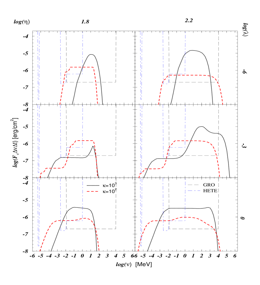
Figure 1: Spectra for $E_{51}=1,\theta=0.1,t_{w}=100\rm{s},t_{var}=40\rm{ms}$, $\eta=63$ (left column), $\eta\approx 160$ ( right column), and for different values of the magnetic field and the electron acceleration efficiency. The long dashed line shows the approximate threshold and window for GRO’s BATSE and EGRET experiments, while the dotted-dashed one is for all the experiments on board HETE.

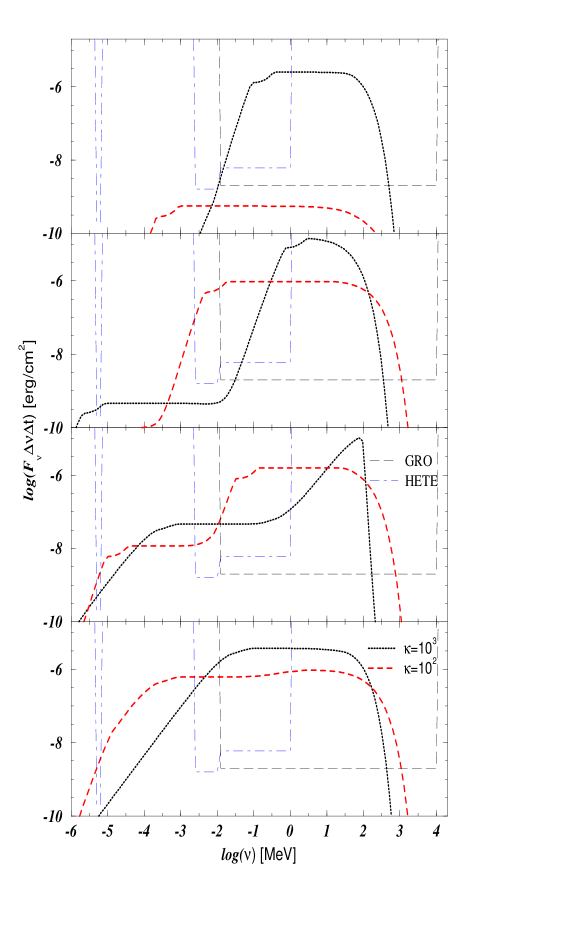
Figure 2: Spectra for $E_{51}=1,\theta=0.1,t_{w}=1\rm{s},t_{var}=40\rm{ms},\eta=200$ and for representative values of the magnetic field (from bottom to top $log(\lambda)=0,-4,-8,-12$) and electron acceleration efficiency. GRO and HETE windows are included.

References

- (1)
- (2)
- Band et al. (1993) Band, D. et al. 1993, ApJ, 413, 281
- Bykov & Mészáros (1996) Bykov, A. M. & Mészáros, P. 1996, ApJ, 461, L37
- Fenimore et al. (1996) Fenimore, E. E., Madras, C. D. & Nayakshin, S. 1996, ApJ, submitted
- Fishman & Meegan (1995) Fishman, G. J. & Meegan, C. A. 1995, ARA&A 33, 415
- Hanlon et al. (1994) Hanlon, L. O. et al. 1994, A & A, 285, 161
- Katz (1994) Katz, J. E. 1994, ApJ, 422, 248
- Mészáros (1995) Mészáros, P. 1995, in Proc. 17th Texas Symp. Rel. Astroph., (NY Acad.Sci.,NY), 759, 440
- Mészáros & Rees (1993) Mészáros, P. & Rees, M. J. 1993, ApJ, 405, 278
- Mészáros & Rees (1994) Mészáros, P. & Rees, M. J. 1994, MNRAS 269, L41.
- Mészáros, Rees & Papathanassiou (1994) Mészáros, P., Rees, M. J. & Papathanassiou, H. 1994 [MRP94], ApJ, 432, 181.
- Norris et al. (1996) Norris, J. et al. 1996, ApJ, 459, 393
- Paczyński & Xu (1994) Paczyński, B., & Xu, G. 1994, ApJ, 427, 708.
- Papathanassiou & Mészáros (1996) Papathanassiou, H. & Mészáros P., [PM96] in preparation.
- Preece et al. (1996) Preece, R. D. et al. 1996, ApJ, in press
- Rees & Mészáros (1992) Rees, M. J. & Mészáros, P. 1992, MNRAS, 258, 41P.
- Rees & Mészáros (1994) Rees, M. J. & Mészáros, P. 1994 [RM94], ApJ, 430, L93.
- Sari et al. (1996) Sari, R., Narayan, R. & Piran, T. 1996, ApJ, in press
- Thompson (1994) Thompson, C. 1994, MNRAS, 270, 480