Bloated Stars as AGN Broad Line Clouds:
The Emission Line Profiles

Abstract

The ‘Bloated Stars Scenario’ proposes that AGN broad line emission originates in the winds or envelopes of bloated stars (BS). Alexander and Netzer (1994) established that $\sim 5\mbox{$\times$}10^{4}$ BSs with dense, decelerating winds can reproduce the observed emission line spectrum and avoid rapid collisional destruction. Here, we use the observed properties of AGN line profiles to further constrain the model parameters. In the BS model, the origin of the broad profiles is the stellar velocity field in the vicinity of the central black hole. We use a detailed photoionization code and a model of the stellar distribution function to calculate the BS emission line profiles and compare them to a large sample of AGN ${\rm C}\,{\sc iv}\,\lambda 1549$, ${\rm C}\,{\sc iii]}\,\lambda 1909$ and ${\rm Mg}\,{\sc ii}\,\lambda 2798$ profiles. We find that the BSs can reproduce the general shape and width of typical AGN profiles as well as the line ratios if (i) The ionizing luminosity to black hole mass ratio is low enough. (ii) The broad line region size is limited by some cutoff mechanism. (iii) The fraction of the BSs in the stellar population falls off roughly as $r^{-2}$. (iv) The wind density and/or velocity are correlated with the black hole mass and ionizing luminosity. Under these conditions the strong tidal forces near the black hole play an important role in determining the line emission properties of the BSs. Some discrepancies remain: the calculated BS profiles tend to have weaker wings than the observed ones, and the differences between the profiles of different lines are somewhat smaller than those observed.

1 Introduction

The observed properties of active galactic nuclei (AGN) lead to the conclusion that the broad line emission originates in numerous small, cold and dense gas concentrations. These objects are labeled “clouds”, although their true nature remains unknown. A basic challenge for any broad line region (BLR) model is to specify the physical mechanism that protects the clouds from rapid disintegration in the AGN’s extreme environment, or else specify a source for their continued replenishment. The bloated stars (BSs) model [Edwards 1980, Mathews 1983, Scoville & Norman 1988, Penston 1988, Kazanas 1989] proposes that the lines are emitted from the winds or mass loss envelopes of giant stars. The star provides both the gravitational confinement and the mass reservoir for replacing the gas that evaporates from the envelope to the interstellar medium (ISM). The BS model is further motivated by the lack of observational evidence for net radial motion in the BLR (e.g. Maoz et al. 1991, Wanders et al. 1995). This is consistent with virialized motion in the gravitational potential of the nucleus.

The BS model was recently studied by Alexander & Netzer (1994, paper I), which used a detailed photoionization code to calculate the emission line spectrum of various simple BS wind models. The integrated emission line spectrum was calculated by combining the line emissivity of the BSs with theoretical models of the stellar distribution function (DF). The properties of the models were compared to the mean AGN line ratios and to estimates of the BLR size and line reddening. The mean observed ${\rm Ly}\alpha$ equivalent width was used to determine the number of BSs and their fraction in the stellar population and to estimate the collisional mass loss rate and its effect on the ISM electron scattering optical depth.

The main result of paper I is that there are BS wind models that can reproduce the emission line ratios to a fair degree with only a small fraction of BS in the stellar population. However, these models do not resemble winds of normal supergiants. The photoionization calculations show that the emission line spectrum is dominated by the conditions at the outer boundary of the line emitting zone of the wind. The successful BS models are those with dense envelopes that have small density gradients. In this case the wind boundary is set by tidal forces near the black hole and by the finite mass of the wind at larger radii. Only $\sim 5\mbox{$\times$}10^{4}$ such BSs ($<1\%$ of the BLR stellar population) are required for reproducing the BLR emission. As a result, the collision rate is reasonably small ($<1\mbox{$M_{\odot}$}$/yr). On the other hand, lower-density models or those with a steep density gradients are ruled out because they emit strong broad forbidden lines, which are not observed in AGN. In addition, their low line emissivity requires orders of magnitude more BSs in the BLR. This leads to rapid collisional destruction, very high mass loss rate and very short BS lifetimes. Even if the BSs are continuously created, the ISM electron scattering optical depth is very large, contrary to what is observed.

In this second part of the work, we combine our line emission calculations with the dynamics of the stellar cluster to obtain the predicted line profiles for the BS model. This provides a second, powerful test that can, when compounded with observed line profiles, put more constraints on this idea. Section 2 describes the components of the model: the BSs, the ionizing continuum, the stellar distribution function and the black hole mass. Section 3 describes the line profile calculations and presents a large sample of observed profiles. In section 4 we compare the profiles of various BS models to the observed ones. A discussion and a summary of our conclusions are presented in section 5.

2 The model

The observed properties of AGN profiles broadly fall into the following categories:

1. The line width distribution in the AGN population.

2. The profile shapes.

3. The differences between profiles of different lines.

4. Profile asymmetries.

5. Profile shifts relative to the systemic redshift.

A successful BLR model should be able to explain all these properties. The BS model, in its current level of detail, does not attempt to explain the profile asymmetries nor the relative line shifts. Nevertheless, even the remaining profile properties set strong constraints on the BS model. We proceed on the premise that the asymmetries and relative shifts can be eventually explained either within the framework of the BS model or by the existence of another line emitting component in the BLR.

The integrated line emission is a spatial average of the line emissivity in the BLR volume, weighted by the stellar density. Consequently, the line ratios do not impose stringent constraints on the spatial distribution of the gas. The line profile, $L_{u}$ ($u$ is the line of sight projection of the 3D velocity $\mn@boldsymbol{v}$), is a finer probe of the BLR structure, since unlike the total emission, it is integrated only over gas which has line of sight velocity $u$.

The motion of the BSs follows the velocity field of the stellar system that surrounds the black hole. The input parameters that are required for calculating the line profiles are the structure of the BS wind, the black hole mass, the stellar DF and the distribution of the BSs in the normal stellar population. A detailed description of these ingredients can be found in paper I. Here we summarize the relevant properties and list the new features that were introduced into the model.

2.1 The bloated stars

There are to date no reliable models for the structure of massive winds in the presence of an intense external radiation field (see however the recent work by Scoville & Norman [Scoville & Norman 1995] and Hartquist et al [Hartquist et al. 1995]). At this stage, our purpose is to understand the conditions that are required for the BSs to be consistent with both the observed BLR properties and the properties of the stellar population. We therefore model the BS by a simple structure with no claim to hydrodynamical self-consistency and without specifying the process that drives the wind. The validity of this approximation was demonstrated in paper I by showing that the line emission does not depend on the wind internal structure, but predominantly on the conditions at the boundary of its line emitting zone. The BS is modeled by two components: a giant star of radius $\mbox{$R_{\star}$}=10^{13}$ cm and a mass of $\mbox{$M_{\star}$}=0.8\mbox{$M_{\odot}$}$, emitting a spherically symmetric wind of radius $R_{\rm w}$ which contains an additional mass of up to $\mbox{$M_{\rm w}$}=0.2\mbox{$M_{\odot}$}$. The wind density and velocity are linked by the continuity equation

$$\mbox{$\dot{M}_{\rm w}$}=4\pi R^{2}v(R)N(R)\,.$$ (1)

where $\mbox{$\dot{M}_{\rm w}$}=10^{-6}\mbox{$M_{\odot}$}$/yr is the mass loss rate and $N$ is the hydrogen number density. The wind structure is parameterized by a power-law velocity field:

$$v(R)=\mbox{$v_{\star}$}(R/\mbox{$R_{\star}$})^{-\alpha}\,,$$ (2)

where $v_{\star}$ is the velocity at the surface of the star. This family of models spans a two-parameter space, $(\alpha,\mbox{$v_{\star}$})$, which was investigated extensively in paper I. Here we will concentrate on the values that best reproduce the observed emission line spectrum, $\alpha=1/2$ (free falling flow) and $\mbox{$v_{\star}$}\sim 10^{4}$ cm/s (slow and dense wind, $10^{8}\mathrel{\mathchoice{\vbox{\offinterlineskip\halign{$\displaystyle\hfil#\hfil$\cr<\crcr\sim\crcr} }}{\vbox{\offinterlineskip\halign{$\textstyle\hfil#\hfil$\cr<\crcr\sim\crcr} }}{\vbox{\offinterlineskip\halign{$\scriptstyle\hfil#\hfil$\cr<\crcr\sim\crcr} }}{\vbox{\offinterlineskip\halign{$\scriptscriptstyle\hfil#\hfil$\cr<\crcr\sim\crcr} }}}N\mathrel{\mathchoice{\vbox{\offinterlineskip\halign{$\displaystyle\hfil#\hfil$\cr<\crcr\sim\crcr} }}{\vbox{\offinterlineskip\halign{$\textstyle\hfil#\hfil$\cr<\crcr\sim\crcr} }}{\vbox{\offinterlineskip\halign{$\scriptstyle\hfil#\hfil$\cr<\crcr\sim\crcr} }}{\vbox{\offinterlineskip\halign{$\scriptscriptstyle\hfil#\hfil$\cr<\crcr\sim\crcr} }}}10^{12}$ cm^-3).

The size of the wind, and hence its boundary density is determined by three competing physical processes. Tidal disruption of the outer layers of the wind by the black hole limits the size of the wind to

$$\mbox{$R_{\rm tidal}$}(r)=X_{\rm tidal}(M_{\star}/\mbox{$M_{\rm bh}$})^{1/3}r\,,$$ (3)

where $M_{\rm bh}$ is the black hole mass, $r$ is the distance from the black hole and $X_{\rm tidal}$ is a factor of order unity (we assume $X_{\rm tidal}=2$). We will use the term “tidally-limited” to designate such BSs. The finite mass in the wind sets an upper limit on the wind size, $R_{\rm mass}$,

$$\int_{\mbox{$R_{\star}$}}^{\mbox{$R_{\rm mass}$}}\frac{\mbox{$\dot{M}_{\rm w}$}}{v}dR=\mbox{$M_{\rm w}$}\,.$$ (4)

We will use the term “mass-limited” to designate such BSs. The third process is Comptonization [Kazanas 1989], whereby the central ionizing continuum heats the outer layers of the wind, ionizes them completely and reduces their optical depth to zero. The radiation penetrates into the denser parts of the wind until the density rises above a critical value $N_{\rm\/C}$, and an ionization equilibrium is established at the Comptonization radius $R_{\rm\/C}$. The emission line spectrum is determined by the ionization parameter, $U$, which is essentially the ratio of the ionizing flux and gas density at the gas surface. The results of paper I show that the gas at the Comptonized wind boundary has a high $U$. This results in strong emission of unobserved forbidden lines, and therefore this process must be suppressed. The high gas density and small density gradient of the slow and dense wind models achieve this suppression by having $\mbox{$R_{\rm\/C}$}>\mbox{$R_{\rm tidal}$}$ or $\mbox{$R_{\rm\/C}$}>\mbox{$R_{\rm mass}$}$.

2.2 The galactic nucleus

The stellar distribution function that we use is based on the numeric results of Murphy, Cohn & Durisen [Murphy, Cohn & Durisen 1991] (henceforth MCD), which follow the evolution of a multi-mass coeval stellar cluster in the presence of a central black hole. The black hole mass grows as it accretes mass from the stars, both directly, by tidal disruption, and indirectly, from mass loss in the course of stellar evolution and of inelastic stellar collisions. The MCD calculations assume spherical symmetry and an initial Plummer DF with a seed black hole of $10^{4}\mbox{$M_{\odot}$}$.

In this work we use MCD model 2B, which has an initial central density of $7\mbox{$\times$}10^{7}\mbox{$M_{\odot}$}$/pc³, $\sim 3\mbox{$\times$}10^{8}\mbox{$M_{\odot}$}$ within the inner 1 pc and a total mass of $\mbox{$M_{\rm sys}$}=8.5\mbox{$\times$}10^{8}\mbox{$M_{\odot}$}$ within 100 pc. The luminosity is due to spherical accretion with rest-mass to luminosity conversion efficiency of 0.1. The luminosity reaches a peak of $2.4\mbox{$\times$}10^{46}$ erg/s at $4\mbox{$\times$}10^{8}$ yr. The black hole reaches a mass of $5.5\mbox{$\times$}10^{8}\mbox{$M_{\odot}$}$ after 15 Gyr. We study this system at two epochs. The first is at $t_{0}=3\mbox{$\times$}10^{8}$ yr, when $\mbox{$M_{\rm bh}$}=8\mbox{$\times$}10^{7}\mbox{$M_{\odot}$}$, $L_{\rm ion}=7\mbox{$\times$}10^{45}$ erg/s and the luminosity is Eddington-limited. This young system, which was the one studied in paper I, has the luminosity of a bright quasar. The second is at $t_{0}=10^{9}$ yr, when $\mbox{$M_{\rm bh}$}=1.9\mbox{$\times$}10^{8}\mbox{$M_{\odot}$}$, $L_{\rm ion}=3.6\mbox{$\times$}10^{44}$, the luminosity is sub-Eddington and determined by the mass loss rate from the stellar system. This evolved system has the luminosity of a luminous Seyfert 1.

MCD assume, for simplicity, that the velocity DF can be approximated by the Maxwell-Boltzmann DF

$${\rm DF}(r,v,t)=\left(\frac{3}{2\pi}\right)^{3/2}\frac{\mbox{$n_{\star}$}(r,t)}{v_{0}(r,t)^{3}}\exp\left[-\frac{3}{2}\left(\frac{v}{v_{0}(r,t)}\right)^{2}\right]\,,$$ (5)

where $n_{\star}$ is the stellar density and $v_{0}$ the r.m.s velocity. Thus, the velocity field is fully specified by $v_{0}(r,t)$, which MCD calculate numerically by following the time evolution of the system.

Our calculations use an approximate $\mbox{$n_{\star}$}(r,t)$, which is based on the density function of the $0.8\mbox{$M_{\odot}$}$ mass bin stars (that being the mass bin closest to $1\mbox{$M_{\odot}$}$ in MCD figure 6, see paper I). The density function $n_{0.8}(r)$ is given in MCD for several values of $t_{0}$. We interpolate it to any $t_{0}$ and then approximate $n_{\star}$ by

$$\mbox{$n_{\star}$}(r,t_{0})=n_{0.8}(r,t_{0})\frac{\mbox{$M_{\rm sys}$}-\mbox{$M_{\rm bh}$}}{\mbox{$M_{\odot}$}4\pi\int r^{\prime 2}n_{0.8}dr^{\prime}}\,,$$ (6)

that is, by approximating that the ratio between the total stellar density and that of the $0.8\mbox{$M_{\odot}$}$ mass bin stars, ($\sim 4$), does not depend on $r$ and that the mean stellar mass is $1\mbox{$M_{\odot}$}$. For $v_{0}(r,t)$ we use a semi-analytic approximation, which is derived from the following arguments. We model the stellar core at times $t_{0}=3\mbox{$\times$}10^{8}$ and $10^{9}$ yr, which are both earlier than the collisional time-scale of the initial Plummer distribution, $t_{\rm c}=1.2$ Gyr. The relevant dynamical length scale in the nucleus is the black hole dynamical radius, $r_{\rm dyn}=G\mbox{$M_{\rm bh}$}/v^{2}_{\rm init}$, where $v_{\rm init}$ is the initial Plummer r.m.s velocity ($v_{\rm init}=1360$ km/s for MCD model 2B). At $r\ll r_{\rm dyn}$, the initial DF evolves rapidly due to the frequent stellar collisions in the deep potential well, so that by $t_{0}$ the velocity field is dominated by the black hole. Consequently, only the black hole mass, rather than the detailed form of $n_{\star}(r,t)$, is required for calculating $v_{0}$. The spatial redistribution of the stellar mass at $r\ll r_{\rm dyn}$, whether by the evolution of the DF or by the growth of the black hole, does not affect the potential at $r>r_{\rm dyn}$ because the mass distribution is spherically symmetric. Consequently, if $t_{0}<t_{\rm c}$, the initial Plummer DF is almost unchanged except for the small evolutionary mass loss. The MCD models assume that the initial mass function is independent of $r$, and therefore the evolutionary mass loss is reflected only in a small, spatially homogeneous decrease of the initial stellar density.

At small $r$, the potential of the black hole dominates and $v_{0}^{2}=\gamma G\mbox{$M_{\rm bh}$}/r$, where $\gamma$ is of order unity. The width of the line profiles strongly depends on $\gamma$ and it is therefore important to estimate it as reliably as possible. Cohn & Kulsrud [Cohn & Kulsrud 1978] find that $\gamma\sim 1.2$ at $0.001<r/r_{\rm dyn}<0.1$. Bahcall & Wolf [Bahcall & Wolf 1976] similarly find that $\gamma\ga 12/11$ at $r<r_{\rm dyn}$ and that it increases by up to a factor of 2 as $r$ decreases. David et al [David, Durisen & Cohn 1987] and MCD (B. Murphy, private communication) find that $\gamma$ approaches 2 as $r$ decreases. This result can be explained qualitatively in terms of the orbits of the stars near the black hole. If these stars were in bound circular Keplerian orbits, $\gamma$ would have been 1. However, such bound stars are quickly destroyed by stellar collisions and tidal disruption. The only stars that can exist at such small radii are those that spend there only a very short fraction of their period and have high enough angular momenta to avoid falling into the black hole. Such orbits are marginally bound, nearly parabolic Keplerian orbits, which have $\gamma=2$. At larger radii the stellar destruction proceeds more slowly, the fraction of bound stars increases and therefore $\gamma$ decreases.

The r.m.s. velocity of the initial Plummer distribution is

$$v_{0}=\sqrt{\frac{\Psi(r)}{2}}\,,$$ (7)

where $\Psi$ is the negative of the gravitational potential

$$\Psi=\frac{G\mbox{$M_{\rm sys}$}}{\sqrt{r_{0}^{2}+r^{2}}}\,,$$ (8)

and $r_{0}=1$ pc is the core radius [Binney & Tremaine 1987]. We propose to approximate the r.m.s velocity by the simplest expression that approaches the correct limits at small and large $r$,

$$v_{0}^{2}(r)=\frac{G(\mbox{$M_{\rm sys}$}-\mbox{$M_{\rm bh}$})}{2\sqrt{r_{0}^{2}+r^{2}}}+\gamma(r)\frac{G\mbox{$M_{\rm bh}$}}{r}\,,$$ (9)

where $\gamma(r)$ is a smooth function that approaches 2 at small radii and 1 at large radii.

We approximate $\gamma(r)$ by assuming that dynamically, the stellar population near the black hole is composed of two types of stars. A fraction $f_{\rm b}$ of the stars are bound to the black hole in circular orbits and have $\gamma_{b}=1$, while the remaining $f_{u}=1-f_{\rm b}$ of the stars are unbound, in parabolic orbits with $\gamma_{u}=2$. We further assume that the velocity distributions of the bound and unbound stars are Maxwellian with $v_{0,b}^{2}$ and $v_{0,u}^{2}$ of the same form as equation 9, with $\gamma_{b}$ and $\gamma_{u}$, respectively. It then follows that the total population has $v_{0}^{2}=f_{b}v_{0,b}^{2}+f_{u}v_{0,u}^{2}$ and that

$$\gamma(r)=f_{b}\gamma_{b}+f_{u}\gamma_{u}=2-f_{b}\,.$$ (10)

We assume that initially all the stars are bound. With time, inelastic collisions and tidal disruption by the black hole deplete the fraction of bound stars. The MCD results show that inelastic stellar collisions is the dominant mass loss process for the high density stellar cores which are studied here. We therefore neglect the tidal disruptions as a mass loss process.

$f_{b}(t_{0})$ is equal to the probability of a bound star to survive up to time $t_{0}$. At each inelastic encounter, which occur at a rate $q_{c}$, the star loses on average a fraction $\kappa$ of its mass. By approximating that the fractional collisional mass loss rate, $\kappa q_{c}$, is constant in time and equal to its value at $t_{0}$, we obtain

$$f_{b}=\exp(-\kappa q_{\rm c}t_{0})\,.$$ (11)

The collisional rate for equal mass and radius stars with a Maxwellian DF is [Binney & Tremaine 1987]

$$q_{\rm c}(t_{0})=16\sqrt{\frac{\pi}{3}}\mbox{$n_{\star}$}v_{0}R_{\star}^{2}\left(1+\frac{3v_{\rm esc}^{2}}{4v_{0}^{2}}\right)\,,$$ (12)

where $R_{\star}$ is the stellar radius, $v_{\rm esc}$ is the escape velocity from the star and the second term in the brackets is the Safronov number, which takes into account the enhancement of the collision rate by gravitational focusing. For $\kappa$ we use the approximate form suggested by MCD,

$$\kappa=\kappa_{\infty}10^{-v_{\rm esc}/v_{0}}\,, \kappa_{\infty}=0.1\,.$$ (13)

Both $q_{\rm c}$ and $\kappa$ are functions of $\gamma$ (through $v_{0}$) and therefore $\gamma(r)$ (equation 10) is the root of the equation

$$\gamma=2-\exp(-\kappa(\gamma)q_{\rm c}(\gamma)t_{0})\,,$$ (14)

which is solved for $\gamma$ numerically.

Figure 1 compares the approximated $v_{0}$ to that calculated by MCD for model 2B at two epochs (B. Murphy, private communication). The approximation tends to under-estimate the velocity at larger $r$ and slightly over-estimate it at small $r$. These trends appear also for the younger or less massive MCD models. However, in all these cases the fractional error in the approximation is less than 10%, which we consider to be well within the joint uncertainties of the BS model and the MCD results.

Finally, we note that BSs are expected to undergo more collisions than the smaller main sequence (MS) stars. It is therefore possible that the BSs will not share the same velocity field as the general stellar population but are all marginally bound with $\gamma=2$. Figure 1 shows that this may result in an increase of up to $\sim 20\%$ in the BS r.m.s velocity in young systems when $t_{0}$ is much smaller than the MS collisional time-scale, but less so in more evolved systems.

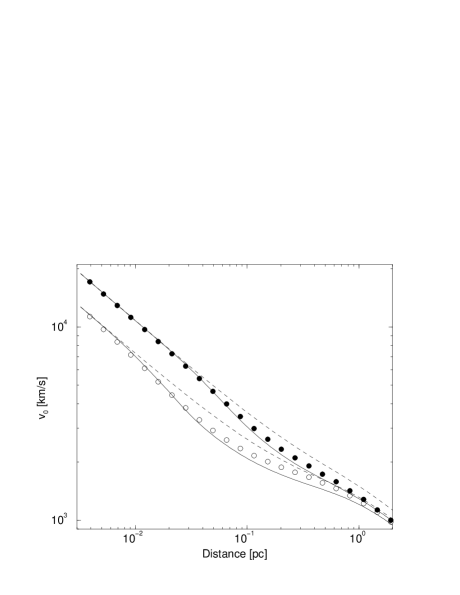
Figure 1: The analytic approximation of the r.m.s stellar velocity, $v_{0}$, compared to the MCD results. Solid line: The approximate $v_{0}$ (equation 9) of the main sequence stars. Dashed line: The approximate $v_{0}$ of the marginally bound ($\gamma=2$) stars only. Open circles: $v_{0}$ calculated by MCD for model 2B at $t_{0}=6.3\mbox{$\times$}10^{7}$ yr, when $\mbox{$M_{\rm bh}$}=6.0\mbox{$\times$}10^{7}\mbox{$M_{\odot}$}$. Full circles: $v_{0}$ calculated by MCD for model 2B at $t_{0}=5.3\mbox{$\times$}10^{8}$ yr, when $\mbox{$M_{\rm bh}$}=1.3\mbox{$\times$}10^{8}\mbox{$M_{\odot}$}$. (Courtesy of B. Murphy)

2.3 New features of the BS model

2.3.1 The fraction of BSs

In paper I, we assumed that the fraction of the BS in the stellar population, $f_{\rm\/BS}$, is constant and independent of $r$. This is obviously only a crude approximation. BSs are not observed in normal stellar environments, such as are, presumably, the host galaxies of AGN. This implies that $f_{\rm\/BS}$ must approach zero at large $r$. The results of section 4 below indicate that the form $\mbox{$f_{\rm\/BS}$}\propto r^{-2}$ may be necessary for reproducing the shape of the observed profiles. We therefore model here also the case of

$$\mbox{$f_{\rm\/BS}$}(r)=\min(f_{\max},f_{\max}\left(\frac{r_{f}}{r}\right)^{2})\,,$$ (15)

where $f_{\max}\leq 1$ is an upper bound on the fraction of BSs in the stellar population and $r_{f}$ is the distance where the BS fraction reaches this bound. $f_{\max}$ is a free parameter of the BS model. We will make the arbitrary assumption that $f_{\max}\sim 1/4$, the fraction of the $0.8\mbox{$M_{\odot}$}$ mass bin stars in the stellar population. For the model discussed below, $v_{0}(r_{f})>10000$ km s^-1. Since BSs with such a high velocity contribute very little to the line emission, for all practical purposes $\mbox{$f_{\rm\/BS}$}\propto r^{-2}$.

2.3.2 Collisional mass loss

Collisional mass loss sets a strong constraint on BS wind models. Reliable estimates of the mass loss rate are especially important for BS distributions that are concentrated towards the black hole. Here we refine the simple estimates used in paper I for the collisional mass loss rate per volume by using equations 12 and 13 and by taking into account the exact amount of mass in the wind, rather than the typical $\mbox{$M_{\rm w}$}=0.2\mbox{$M_{\odot}$}$. Thus, for BS–BS collisions

$$\dot{\rho}_{\rm BS\,coll}(r) = \mbox{$f_{\rm\/BS}$}(r)\mbox{$n_{\star}$}(r)[q_{{\rm c},\star}\kappa_{\star}\mbox{$M_{\star}$}+$$

$$(q_{\rm c,w}-q_{{\rm c},\star})\kappa_{\rm w}\mbox{$M_{\rm w}$}(\mbox{$R_{\rm w}$})]\,,$$

where the collisions of the giant star and of the wind are treated separately, $q_{\rm c,\star}$ and $\kappa_{\star}$ are calculated with $M_{\star}$, $R_{\star}$ and $q_{\rm c,w}$ and $\kappa_{\rm w}$ are calculated with $\mbox{$M_{\star}$}+\mbox{$M_{\rm w}$}(\mbox{$R_{\rm w}$})$, $R_{\rm w}$. Similarly, for the MS–MS collisions

$$\dot{\rho}_{\rm MS\,coll}(r)=[1-\mbox{$f_{\rm\/BS}$}(r)]\mbox{$n_{\star}$}(r)q_{\rm c}\kappa\mbox{$M_{\odot}$}\,,$$ (17)

where $q_{\rm c}$ and $\kappa$ are calculated with 1 $M_{\odot}$ and 1 $R_{\odot}$.

2.3.3 Reddening correction

The amount of intrinsic reddening in AGN spectra is still an unresolved issue [MacAlpine 1985, Netzer 1990]. We assume the “screen hypothesis”, whereby the dust lies just outside the line emitting region and intercepts all the observed spectrum, continuum as well as lines. In paper I we estimated the extinction coefficient, $E_{\rm\/B-V}$, from the difference between the calculated and the mean observed ${\rm Ly}\alpha/{\rm H}\beta$ ratio. We then corrected all the other lines accordingly. This procedure does not allow for the fact that there is actually a range of observed ${\rm Ly}\alpha/{\rm H}\beta$ ratios. It is also vulnerable to possible inaccuracies in the ${\rm Ly}\alpha$ and ${\rm H}\beta$ radiative transfer method that is used by the photoionization code. This was not a serious problem in paper I, since the models that succeeded in reproducing the emission line spectrum required only a small reddening correction, while the other models were ruled out by excessive collisional mass-loss. Here we relax the reddening criterion and determine $E_{\rm\/B-V}$ within the range 0 to $\mbox{$E_{\rm\/B-V}$}({\rm Ly}\alpha/{\rm H}\beta)$ by a $\chi^{2}$ fit of all the calculated line ratios and their mean observed values (table 1 in paper I).

3 Theoretical and observed line profiles

3.1 Theoretical line profiles

The basic output of the photoionization calculations is $L_{\ell}(r)$, the luminosity in a given line from a single BS at a distance $r$. The numerical procedure for calculating $L_{\ell}(r)$ for a given BS wind density structure, chemical composition and the ionizing flux spectrum is as described in paper I.

$L_{u}$, the differential line luminosity per line of sight velocity $u$, is given by

$$L_{u} = \int^{\mbox{$r_{\rm out}$}}_{\mbox{$r_{\rm in}$}}drr^{2}\int^{4\pi}_{0}d\Omega_{r}\int^{v_{\max}(r)}_{0}dvv^{2}\int^{4\pi}_{0}d\Omega_{v}\times$$ (18)

$$L_{\ell}(r){\rm DF}(\mn@boldsymbol{r},\mn@boldsymbol{v})\delta(v\mu_{r}-u)\,,$$

where ${\rm DF}(\mn@boldsymbol{r},\mn@boldsymbol{v})$ is the BS distribution function and $v_{\max}(r)$ is the maximal stellar velocity at distance r from the black hole. For an isotropic stellar distribution with an isotropic velocity field, ${\rm DF}(\mn@boldsymbol{r},\mn@boldsymbol{v})={\rm DF}(r,v)$, $L_{u}$ reduces to

$$L_{u}=8\pi^{2}\int^{r_{2}}_{r_{1}}drr^{2}L_{\ell}(r)\int^{v_{\max}(r)}_{|u|}dv|v|{\rm DF}(r,v)\,,$$ (19)

where the $\delta$ function is translated into the integration range $(r_{1},r_{2})$, which is the sub-interval of $(\mbox{$r_{\rm in}$},\mbox{$r_{\rm out}$})$ where $|u|\leq v_{\max}(r)$. For the assumed Maxwell-Boltzmann velocity field (equation 5) $v_{\max}(r)\rightarrow\infty$ and the line profile is

$$L_{u} = \sqrt{24\pi}\int^{\mbox{$r_{\rm out}$}}_{\mbox{$r_{\rm in}$}}drr^{2}L_{\ell}(r)\frac{n_{\star}(r)}{v_{0}(r)}\exp\left[-\frac{3}{2}\left(\frac{u}{v_{0}(r)}\right)^{2}\right]\,.$$

Equation 3.1, together with the $L_{\ell}(r)$ results of the photoionization calculation and the approximate $v_{0}(r)$ (equation 9), are used below to predict the line profiles of several different BS models.

3.2 Observed line profiles

The calculated line profiles are compared to a sample of 87 ${\rm C}\,{\sc iii]}\,\lambda 1909$ profiles, 140 ${\rm C}\,{\sc iv}\,\lambda 1549$ profiles and 72 ${\rm Mg}\,{\sc ii}\,\lambda 2798$ profiles, for which we measured the full line widths (FW) at 1/4, 1/2 and 3/4 of the maximum height. This sample was compiled from several sources. 111 of the ${\rm C}\,{\sc iv}\,\lambda 1549$ lines are from an absorption line survey of 123 high luminosity AGN [Sargent, Boksenberg & Steidel 1988, Sargent, Steidel & Boksenberg 1989, Sargent & Steidel 1995], which were selected by apparent magnitude and redshift. The QSO lie primarily in the redshift range $z\sim 1.9$ to $3.5$ and the in the absolute magnitude range $M_{V}\sim-32$ to $-27$. The continuum subtracted spectra of this sample, which were measured here, are from Wills et al [Wills et al. 1993]. The ${\rm C}\,{\sc iii]}\,\lambda 1909$ and ${\rm Mg}\,{\sc ii}\,\lambda 2798$ and 29 of the ${\rm C}\,{\sc iv}\,\lambda 1549$ profiles are from a sample of 42 radio-selected QSO and 50 radio-quiet QSO, which were selected by UV excess or slitless spectroscopy [Steidel & Sargent 1991]. The QSO lie primarily in the redshift range $z\sim 0.9$ to $2.2$ and in the rest-frame monochromatic absolute magnitude range $M(\lambda 2200{\rm\AA})\sim-30$ to $-26$. The continuum subtracted spectra of this sample, which were measured here, are from Brotherton et al [Brotherton et al. 1994a]. All the continuum subtracted spectra were kindly supplied by M. Brotherton.

Figure 2: The average observed ${\rm C}\,{\sc iv}\,\lambda 1549$, ${\rm C}\,{\sc iii]}\,\lambda 1909$ and ${\rm Mg}\,{\sc ii}\,\lambda 2798$ profiles, weighted by the integrated flux. The ${\rm Mg}\,{\sc ii}\,\lambda 2798$ profile is shown both with and without the assumed ${\rm Fe}\,{\sc ii}\,$ contribution.

We are interested in studying the shape of the line profiles, which requires information on the line width at several heights. A common procedure for measuring the FW of a spectral line is to fit the profile to a superposition of several Gaussians and measure the width of the smooth fitted function. This procedure is also used to deblend adjacent spectral lines from the profile. Since we are interested in the large sample statistics rather than the properties of a specific AGN, and since the art of multi-Gaussian fitting has a strong subjective element in it even under optimal conditions, we decided to adopt a simpler procedure. We rely on the fact that all lines of interest are much stronger than neighbouring lines and do not attempt any deblending or fitting, but simply located “by eye” the profile peak and underlying continuum level. In cases where the blended line was clearly visible, we adjusted the FW “by eye” accordingly. In cases where the spectrum was very noisy, we smoothed it by averaging the flux in overlapping windows of $n$ consecutive pixels (usually $n=5$).

The measurement of the ${\rm Mg}\,{\sc ii}\,\lambda 2798$ FW is complicated by the fact that this line is blended with a number of ${\rm Fe}\,{\sc ii}\,$ lines, which add to the ${\rm Mg}\,{\sc ii}\,\lambda 2798$ profile wide and flat broad wings [Wills, Netzer & Wills 1985]. Since it is not our intention to do here a careful deblending of the ${\rm Mg}\,{\sc ii}\,\lambda 2798$ profile, we measured the ${\rm Mg}\,{\sc ii}\,\lambda 2798$ twice, once with these wings and once without them. In the latter case, only 68 profiles were measured since the others lacked distinct wings. These two types of measurements, which we designate by ${\rm Mg}\,{\sc ii}\,\lambda 2798{\rm+}{\rm Fe}\,{\sc ii}\,$ and ${\rm Mg}\,{\sc ii}\,\lambda 2798{\rm-}{\rm Fe}\,{\sc ii}\,$, respectively, represent the two extreme assumptions that either the wings are all ${\rm Mg}\,{\sc ii}\,\lambda 2798$ emission or that only the line core is ${\rm Mg}\,{\sc ii}\,\lambda 2798$ emission. Thus, a BLR model that predicts FW(Mg ii $\lambda 2798$) $\ll$ FW(Mg ii $\lambda 2798$-${\rm Fe}\,{\sc ii}\,$) or FW(Mg ii $\lambda 2798$) $\gg$ FW(Mg ii $\lambda 2798$+${\rm Fe}\,{\sc ii}\,$) is inconsistent with the observations.

We compared our FWHM results with the Gaussian fit results of Wills et al [Wills et al. 1993] and Brotherton et al [Brotherton et al. 1994a] by calculating the mean fractional difference, $(\mbox{\rm FWHM}_{\mbox{\rm by eye}}-\mbox{FWHM}_{\mbox{\rm gauss}})/\mbox{FWHM}_{\mbox{\rm gauss}}$, and its rms scatter. For the ${\rm C}\,{\sc iv}\,\lambda 1549$, ${\rm C}\,{\sc iii]}\,\lambda 1909$, ${\rm Mg}\,{\sc ii}\,\lambda 2798{\rm+}{\rm Fe}\,{\sc ii}\,$ and ${\rm Mg}\,{\sc ii}\,\lambda 2798{\rm-}{\rm Fe}\,{\sc ii}\,$ profiles the mean fractional differences are $-0.009\pm 0.06$, $0.05\pm 0.15$, $-0.01\pm 0.1$ and $-0.26\pm 0.13$, respectively. The correspondence of the two methods for the ${\rm C}\,{\sc iv}\,\lambda 1549$ and ${\rm Mg}\,{\sc ii}\,\lambda 2798{\rm+}{\rm Fe}\,{\sc ii}\,$ lines is very good. The relatively larger over-estimation of the ${\rm C}\,{\sc iii]}\,\lambda 1909$ FWHM is due to the blended ${\rm Al}\,{\sc iii}\,\lambda 1859$ and the big difference in ${\rm Mg}\,{\sc ii}\,\lambda 2798{\rm-}{\rm Fe}\,{\sc ii}\,$ is due to the fact that Wills et al [Wills et al. 1993] and Brotherton et al [Brotherton et al. 1994a] did not deblend the ${\rm Fe}\,{\sc ii}\,$ contribution to the ${\rm Mg}\,{\sc ii}\,\lambda 2798$ profile.

Figure 2 shows the sample averaged profiles, where the profiles are weighted by their inverse integrated flux. It should be noted that other weighing methods (e.g. by the peak flux), or other averaging procedures (e.g. averaging the blue and red half widths at $x$% of the maximum, for $x=0$ to 100%) yield very different results. This ambiguity indicates that the average profile is not a very useful quantity and that the calculated profiles should be evaluated by the cumulative distribution function or on an object to object basis. Figure 3 shows the FW cumulative distribution functions of the three lines at 1/4, 1/2 and 3/4 maximum.

Figure 3: The cumulative distribution functions of the observed FW at 1/4, 1/2 and 3/4 maximum for ${\rm C}\,{\sc iv}\,\lambda 1549$, ${\rm C}\,{\sc iii]}\,\lambda 1909$ and ${\rm Mg}\,{\sc ii}\,\lambda 2798$. The QSO number density per FW interval is proportional to the density of vertical lines. The ${\rm Mg}\,{\sc ii}\,\lambda 2798$ cumulative FW distribution is based on the ${\rm Mg}\,{\sc ii}\,\lambda 2798{\rm+}{\rm Fe}\,{\sc ii}\,$ measurements. The ${\rm Mg}\,{\sc ii}\,\lambda 2798{\rm-}{\rm Fe}\,{\sc ii}\,$ distribution is outlined by the bold line.

4 Results

We investigate the line profiles of the BS model by studying a succession of three BS wind / stellar DF models, whose properties are summarised in table 1. Model A is similar to that studied in paper I. We show below that in order to reproduce the observed line profiles and ratios, some changes in the model assumptions are required. These changes are introduced in two steps, in models B and C.

	Model A	Model B	Model C
$v_{\star}$	$5\mbox{$\times$}10^{3}$ cm s-1	$8\mbox{$\times$}10^{4}$ cm s-1	$8\mbox{$\times$}10^{4}$ cm s-1
$M_{\rm bh}$	$8.0\mbox{$\times$}10^{7}\mbox{$M_{\odot}$}$	$1.9\mbox{$\times$}10^{8}\mbox{$M_{\odot}$}$	$1.9\mbox{$\times$}10^{8}\mbox{$M_{\odot}$}$
$t_{0}$	$3\mbox{$\times$}10^{8}$ yr	$10^{9}$ yr	$10^{9}$ yr
$L_{\rm ion}$	$7\mbox{$\times$}10^{45}$ erg s-1	$3.6\mbox{$\times$}10^{44}$ erg s-1	$3.6\mbox{$\times$}10^{44}$ erg s-1
$r_{\rm in}$	0.001 pc	0.001 pc	0.001 pc
$r_{\rm out}$	1 pc	0.25 pc	0.25 pc
No. of BSs	$1.5\mbox{$\times$}10^{5}$	$4.3\mbox{$\times$}10^{4}$	$4.7\mbox{$\times$}10^{4}$
Fraction of BSs	$4.7\mbox{$\times$}10^{-4}$	$2.4\mbox{$\times$}10^{-3}$	$2.6\mbox{$\times$}10^{-3}$
$f_{\rm\/BS}$	$\propto r^{0}$	$\propto r^{0}$	$\propto r^{-2}$
$\dot{M}_{\rm evol}$	$0.15\mbox{$M_{\odot}$}$ yr-1	$4.3\mbox{$\times$}10^{-2}\mbox{$M_{\odot}$}$ yr-1	$4.8\mbox{$\times$}10^{-2}\mbox{$M_{\odot}$}$ yr-1
$\dot{M}_{\rm BS\,coll}$	$3.2\mbox{$M_{\odot}$}$ yr-1	$0.37\mbox{$M_{\odot}$}$ yr-1	$0.59\mbox{$M_{\odot}$}$ yr-1
$\dot{M}_{\rm MS\,coll}$	$2.8\mbox{$\times$}10^{-2}\mbox{$M_{\odot}$}$ yr-1	$1.1\mbox{$\times$}10^{-2}\mbox{$M_{\odot}$}$ yr-1	$1.1\mbox{$\times$}10^{-2}\mbox{$M_{\odot}$}$ yr-1
Electron scattering $\dot{\tau}$	$<3.8\mbox{$\times$}10^{-4}$ yr-1	$<1.8\mbox{$\times$}10^{-4}$ yr-1	$<0.08$ yr-1
$E_{\rm\/B-V}$	0.066	0.000	0.096
${\rm Ly}\alpha$ flux weighted radius	493 ld	209 ld	25 ld

Table 1: The parameters and calculated properties of models A, B and C. The growth rate of the electron scattering optical depth, $\dot{\tau}$, is estimated under the assumption that all the mass accumulates in the BLR and is neither accreted nor ejected (see paper I).

4.1 Model A

We begin by considering the successful BS model of paper I (hereafter model A, see table 1), which has the BS wind parameters $\alpha=1/2$ and $\mbox{$v_{\star}$}=5\mbox{$\times$}10^{3}$ cm/s, an AGN model of $\mbox{$M_{\rm bh}$}=8\mbox{$\times$}10^{7}\mbox{$M_{\odot}$}$ and $\mbox{$L_{\rm ion}$}=7\mbox{$\times$}10^{45}$ erg/s at $t_{0}=3\mbox{$\times$}10^{8}$ yr and $\mbox{$f_{\rm\/BS}$}={\rm const}$. A free parameter of the model is the BLR size, $r_{\rm out}$. As was shown in paper I, the line spectrum depends only weakly on $r_{\rm out}$ in the range 1/3 pc to $\sim 50$ pc. This is not the case for the line width, which decreases significantly with $r_{\rm out}$. We will assume that the BLR outer limit scales as $\mbox{$r_{\rm out}$}\sim(\mbox{$L_{\rm ion}$}/10^{46}{\rm erg/s})^{1/2}$ pc. This is motivated both by the line reverberation results that suggest that the average BLR radius is $\sim 0.1(\mbox{$L_{\rm ion}$}/10^{46}{\rm erg/s})^{1/2}$pc [Netzer 1990] and by the possibility that the line emission is suppressed by dust at the dust sublimation radius $r_{\rm sub}\simeq 0.3(\mbox{$L_{\rm ion}$}/10^{46}{\rm erg/s})^{1/2}$pc [Netzer & Laor 1993]. We therefore set $\mbox{$r_{\rm out}$}=1$ pc for model A.

Figure 4 shows some profiles calculated for a BLR size $\mbox{$r_{\rm out}$}=1$ pc. Three properties are immediately apparent: The profiles are very narrow (FWHM $\sim 2200$ km/s), the wings are very weak and the different lines have almost identical profiles, unlike the observed ones (Figure 2). Table 2 shows that only a few percent of the objects in the sample have FWHM as narrow as those calculated, and none have such narrow FW1/4M. We explored also the possibility of reducing $r_{\rm out}$ to 1/3 pc. This increased the ${\rm C}\,{\sc iv}\,\lambda 1549$ FW to 1877 ($\geq 29\%$ of the sample), 2982 ($\geq 14\%$) and 4422 ($\geq 5\%$) km/s for the FW3/4M, FW1/2M and FW1/4M, respectively. However, this modest increase in FW1/4M comes at the price of an excessive BS–BS collisional mass loss rate of $4.5\mbox{$M_{\odot}$}$/yr. As will be discussed below, the emissivity of tidally-limited BSs is approximately independent of $r$. Decreasing the BLR size therefore means that the same number of BS must share a smaller volume and this leads to an increased collision rate.

	Model A			Model B			Model C
FW	${\rm C}\,{\sc iv}\,\lambda 1549$	${\rm C}\,{\sc iii]}\,\lambda 1909$	${\rm Mg}\,{\sc ii}\,\lambda 2798$	${\rm C}\,{\sc iv}\,\lambda 1549$	${\rm C}\,{\sc iii]}\,\lambda 1909$	${\rm Mg}\,{\sc ii}\,\lambda 2798$	${\rm C}\,{\sc iv}\,\lambda 1549$	${\rm C}\,{\sc iii]}\,\lambda 1909$	${\rm Mg}\,{\sc ii}\,\lambda 2798$
3/4M	1337	1407	1252	2398	2426	2366	2854	2958	2729
%	(4)	(8)	(1/5)	(49)	(38)	(54/91)	(61)	(47)	(76/96)
1/2M	2090	2202	1952	3734	3789	3709	4561	4782	4319
%	(2)	(2)	(0/3)	(33)	(15)	(41/84)	(48)	(31)	(62/89)
1/4M	2988	3164	2783	5372	5464	5813	6928	7344	6424
%	(0)	(0)	(0/0)	(12)	(2)	(16/86)	(32)	(23)	(20/90)

Table 2: Comparison of the calculated FW to the observed cumulative FW distribution. The FW are in km/s. The numbers in brackets below each FW entry are the percentage of objects in the sample with FW less or equal to the calculated one. For the ${\rm Mg}\,{\sc ii}\,\lambda 2798$, the percentage on the left is based on the ${\rm Mg}\,{\sc ii}\,\lambda 2798{\rm+}{\rm Fe}\,{\sc ii}\,$ FW measurements, and that on the right on the ${\rm Mg}\,{\sc ii}\,\lambda 2798{\rm-}{\rm Fe}\,{\sc ii}\,$ FW measurements.

4.2 Model B

A possible remedy for the width problem is to model a more evolved AGN with a more massive black hole. The MCD models indicate, that apart for a very short initial epoch of Eddington limited accretion, the luminosity decreases with time as the available mass is exhausted (MCD figure 10). The resulting decrease in $r_{\rm out}$ also helps to broaden the profiles. We therefore consider an AGN model at $t_{0}=1$ Gyr, when $\mbox{$M_{\rm bh}$}=1.9\mbox{$\times$}10^{8}\mbox{$M_{\odot}$}$, $\mbox{$L_{\rm ion}$}=3.6\mbox{$\times$}10^{44}$ erg/s and $\mbox{$r_{\rm out}$}=1/4$ pc (hereafter model B, see table 1). As is explained in the appendix, changing $M_{\rm bh}$ and $L_{\rm ion}$ from the values of model A to those of model B worsens the fit of the calculated line ratios to the observed ones, unless accompanied by a suitable modification of the wind parameters. In paper I, we systematically searched the BS wind parameter space for the values that best reproduce the observed line ratios. Here, we use instead the scaling prescription given in the appendix, which shows that the line spectrum of model A can be approximately reproduced by modifying the wind velocity to $\mbox{$v_{\star}$}=8\mbox{$\times$}10^{4}$ cm/s. For the continuum spectrum we use the same spectral distribution as used for model A, scaled down to the lower $L_{\rm ion}$ of model B.

The calculated BS–BS collisional mass loss rate of model B is only $0.4\mbox{$M_{\odot}$}$/yr, in spite of the small BLR size. This reflects the fact that most of the mass loss is from collisions of the winds, and that the BS wind density is proportional to $\mbox{$\dot{M}_{\rm w}$}/\mbox{$v_{\star}$}$ (equation 4). Since $R_{\rm tidal}$ is a weak function of $M_{\rm bh}$, the BS wind mass in model B is $\sim 16$ times smaller than that of model A, and so are the respective mass loss rates. Figure 4 and table 2 show that the profiles of model B are indeed wider than those of model A, but the profiles of the three lines are almost identical and the wings are too weak.

Figure 4: The theoretical ${\rm C}\,{\sc iv}\,\lambda 1549$, ${\rm C}\,{\sc iii]}\,\lambda 1909$ and ${\rm Mg}\,{\sc ii}\,\lambda 2798$ profiles for models A, B and C. The model B numerical profiles are fitted to the analytical approximation $L_{u}\propto u^{-6}$ (bold dash-dotted line). The model C numerical profiles are fitted to the analytical approximation $L_{u}\propto u^{-2}$ (bold dash-dotted line).

So far, we assumed that the fraction of BSs in the central cluster, $f_{\rm\/BS}$, is independent of $r$. There are, however, good reasons to modify this approach, both from theoretical considerations and from careful examination of the line wings. As noted by Penston, Croft, Basi & Fuller [Penston, Croft, Basu & Fuller 1990], the far wings of many observed profiles are well fitted by an inverse quadratic form of $F_{\lambda}\propto 1/(\lambda-\lambda_{0})^{2}$ and show that this is consistent with line emission from an ensemble of clouds of constant cross section, moving on parabolic orbits. Here, we extend their analysis to the BSs and show that the discrepancy between the observed wing shapes and those of model B can be explained in terms of the line emissivity from marginally bound BSs.

Let us assume for simplicity that the Maxwellian DF (equation 5) can be approximated by

$$DF(r,v)=\mbox{$f_{\rm\/BS}$}(r)\mbox{$n_{\star}$}(r)\frac{\delta[v-v_{0}(r)]}{4\pi v^{2}}\,,$$ (21)

where $v_{0}^{2}=2G\mbox{$M_{\rm bh}$}/r$. It then follows from equation 19 that

$$L_{u}=2\pi\int_{r_{1}}^{r_{2}}drr^{2}L_{\ell}(r)\mbox{$f_{\rm\/BS}$}(r)\mbox{$n_{\star}$}(r)v_{0}^{-1}(r)\,,$$ (22)

where the upper integration limit is defined by $r_{2}=\min(2G\mbox{$M_{\rm bh}$}/u^{2},\mbox{$r_{\rm out}$})$ and $r_{2}\gg r_{1}$. As explained earlier, marginally bound stars have $v_{0}(r)\propto r^{-1/2}$. Assume that $L_{\ell}(r)\propto r^{-a}$, $\mbox{$f_{\rm\/BS}$}(r)\propto r^{-b}$ and $\mbox{$n_{\star}$}(r)\propto r^{-c}$. It then follows that

$$L_{u}\propto r_{2}^{7/2-(a+b+c)}\,.$$ (23)

At the profile wings $u$ is large enough so that $r_{2}<\mbox{$r_{\rm out}$}$, $r\propto u^{-2}$ and the profile shape is

$$L_{u}\propto u^{-7+2(a+b+c)}\,.$$ (24)

The tidally-limited BSs are dense and optically thick enough, so that their total emissivity is roughly proportional to the product of their geometrical cross-section, $\pi R^{2}_{\rm tidal}\propto r^{2}$ (equation 3) and the central irradiating flux, $F\propto r^{-2}$, and is therefore constant. Figure 5 shows the BS line and total emissivity of model B. The total emitted heat (including all lines and diffuse continua) is indeed very nearly constant .This, however is not true for the individual lines (Fig. 5), whose emissivity depends on the gas density, ionization level and optical depth. Nevertheless, let us make the approximation that $L_{\ell}\sim{\rm const.}$ ($a=0$) and assume also that $\mbox{$f_{\rm\/BS}$}={\rm const.}$ ($b=0$). Marginally bound stars have $\mbox{$n_{\star}$}(r)\propto r^{-1/2}$ $(c=-1/2)$ (e.g. Penston et al 1990). The profile wing is therefore expected to fall off sharply as $L_{u}\propto u^{-6}$. Figure 4 shows that the calculated profiles of model B are well fitted by this expression at high $u$, thereby also justifying the approximation of the DF by the $\delta$ function.

Figure 5: The line emissivity of a single BS, $L_{\ell}$, for models B and C in various lines, as function of the distance from the black hole. The total heat includes all the reprocessed radiation emitted in lines and continuum radiation.

4.3 Model C

4.3.1 Line profiles

Equation 24 and the observed profiles suggest that in order to reproduce the observed inverse quadratic wings, it is necessary to modify some of the model assumptions, so that $a+b+c=5/2$. Changing the BS emissivity by modifying the wind structure will change the emission line spectrum, as shown in paper I. The $r$ dependence of the stellar DF is based on a well established result. The only remaining free parameter is $f_{\rm\/BS}$. If we assume $\mbox{$f_{\rm\/BS}$}\propto r^{-2}$ then the profile wings will have the required shape.

Model C (table 1) has the same parameters as model B but with $\mbox{$f_{\rm\/BS}$}\propto r^{-2}$ (equation 15). Figure 4 and table 2 show that with this choice, the calculated FWHM are representative of the observed sample. However, the percentiles decrease from the FW3/4M to FW1/2M to FW1/4M, indicating that the calculated wings are still somewhat weaker than the observed ones. The calculated ${\rm Mg}\,{\sc ii}\,\lambda 2798$ FW3/4M is now in fact wider than more than 76% percent of the sample profiles. The fit to $L_{u}\propto u^{-2}$, shown in figure 4 is not perfect. This is due to the fact that $L_{\ell}$ of those lines is not constant. We have examined the fit to the calculated ${\rm Ly}\alpha$ profile and found that for this line, whose emissivity is closer to being constant with $r$, The fit of the far wings to $L_{u}\propto u^{-2}$ is very good.

The FWHM ratios of the calculated lines of model C are ${\rm C}\,{\sc iii]}\,\lambda 1909/{\rm C}\,{\sc iv}\,\lambda 1549=1.05$, ${\rm Mg}\,{\sc ii}\,\lambda 2798/{\rm C}\,{\sc iv}\,\lambda 1549=0.95$ and ${\rm Mg}\,{\sc ii}\,\lambda 2798/{\rm C}\,{\sc iii]}\,\lambda 1909=0.90$. These values can be compared to the observed values quoted in Brotherton et al (1994), $1.21\pm 0.04$, $0.97\pm 0.06$ and $0.85\pm 0.05$, respectively. It is apparent that the model ${\rm C}\,{\sc iii]}\,\lambda 1909$ tends to be narrower than the observed one, as is also indicated by the percentages in table 2. Figure 6 demonstrates that there are AGN which have profiles that are very similar to those of model C.

Figure 6: Examples of observed profiles (solid line) which are well fitted by model C (dotted line).

4.3.2 Line ratios

Having established a good agreement between the observed and calculated profiles, we now further test model C by returning to the issues studied in paper I, namely the line ratios and the required number of BSs. The integrated line spectra of models A and C are compared to the mean observed one (paper I, table 1) in figure 8. (Note the similarity between the line ratios of models A and C, which demonstrates that the scaling prescription of the appendix works). The ${\rm Mg}\,{\sc ii}\,\lambda 2798$ and ${\rm N}\,{\sc v}\,\lambda 1240$ deficiencies, which are discussed in paper I, remain a problem. Model C has a slightly high ${\rm[O}\,{\sc iii]}\,\lambda 4363$ emission, which is due to the fact that the scaling only deals with the tidally-limited BSs. At large $r$ the BS are mass-limited. The lower wind gas density of model C implies a larger $R_{\rm mass}$ and consequently a lower density, a larger $U(\mbox{$R_{\rm mass}$})$ and a stronger emission of forbidden lines. The unreddened and reddened spectra of model C are compared to a mean QSO spectrum in figure 7.

Figure 7: The unreddened (dashed line) and reddened, $\mbox{$E_{\rm\/B-V}$}=0.096$, (solid line) spectrum of model C compared with an average observed QSO spectrum (dotted line).

Figure 8: The integrated line ratios of models A ($\triangle$) and C ($\Box$), expressed relative to the ${\rm Ly}\alpha$ luminosity and compared to the observed range (paper I, table 1). The mean observed ratios are indicated by the black dot and the ranges by the error bars. $\mbox{$E_{\rm\/B-V}$}({\rm A})=0.066$ and $\mbox{$r_{\rm out}$}({\rm A})=1$ pc. $\mbox{$E_{\rm\/B-V}$}({\rm C})=0.096$ and $\mbox{$r_{\rm out}$}({\rm C})=1/4$ pc.

Model C is quite successful in reproducing the BLR emission properties. The line ratios, line profiles and BLR size, as estimated by the flux weighted radius of the ${\rm Ly}\alpha$. The total mass loss rate is consistent with the theoretical estimates of the accretion rate and the resulting electron scattering optical depth growth is consistent with the observations of rapid X-ray variability.

5 Discussion and conclusions

The results of paper I indicate that in order to reproduce the integrated emission line spectrum, the BSs should have dense, decelerating winds, whose boundary is not fixed by comptonization. The BLR line profiles are another observed property that the BS model has to reproduce. We find that this imposes additional constraints on the model.

The FW statistics of the observed profiles indicate that the high $L_{\rm ion}/\mbox{$M_{\rm bh}$}$ models that were successful in reproducing the emission line spectrum have too narrow FWs. Observed AGN with such narrow broad lines constitute only a marginal percentage of the sample. Another potential problem with these models is the rather high collisional mass loss rate. The narrow calculated FWs indicate that either $M_{\rm bh}$ should be larger and/or the BLR size smaller. The MCD models of the AGN evolution link the increase in the black hole mass with a decrease in the luminosity (in the post-Eddington limited accretion epoch). The change in the luminosity affects the model properties in two different ways. First, it may decrease the BLR size, since it is natural, although not necessary, to assume that the luminosity determines the BLR size by creating a dust-free inner region which can emit lines. Second, the reduced BLR size and increased black hole mass make the tidally-limited BSs the main contributors to the line emission. We find that, in order to obtain the observed line spectrum from tidally-limited BSs, it is necessary to scale $\mbox{$\dot{M}_{\rm w}$}/\mbox{$v_{\star}$}$ in proportion to $\mbox{$L_{\rm ion}$}/\sqrt{\mbox{$M_{\rm bh}$}}$ (see the appendix). This in turn reduces the wind mass and allows the BSs to survive the increased collisional rate in the smaller, faster moving BLR. The lower $L_{\rm ion}/\mbox{$M_{\rm bh}$}$ models have much wider profiles, which are consistent with the observations. However the far wings are very weak and the profiles of the different species are very similar to each other, contrary to the observed situation.

Although the profile widths of model A are much smaller than those of the sample presented here, we note that there exists a sub-population of narrow line Seyfert 1 galaxies, which are characterized by soft X-ray spectra and comprise about 10% of optically selected Seyfert 1s and 15–50% of soft X-rays selected Seyfert 1s [Boller, Brandt & Fink 1995, Laor et al 1994]. Such AGN have FWHM(${\rm H}\beta$) in the range $\sim$ 500–1500 km/s, which is similar to, or even narrower than the FWHM of model A.

The idea that the inverse quadratic far wings, which are observed in many profiles, are linked to parabolic orbits and to $r^{-2}$ emissivity dependence, was discussed by several authors. The dense and deep potential well in the AGN offers a ‘natural selection’ process which favors such orbits for the BSs, since all the tightly bound BSs are destroyed by collisions or tidal disruptions. The analytic work of Penston et al [Penston, Croft, Basu & Fuller 1990] assumed strictly parabolic orbits and a cloud line emissivity that falls off as $r^{-2}$. Our numeric results confirm that their analysis also holds for a distribution of binding energies around $E=0$. However, unlike their assumed cloud emissivity, the total line emissivity from a single BS is nearly constant in $r$. If we assume that the BSs are a fixed proportion of the normal stellar population, the resulting line profiles are core dominated with very weak wings. This situation can be corrected by relaxing this assumption and setting $\mbox{$f_{\rm\/BS}$}\propto r^{-2}$. The resulting profiles are only approximately inverse quadratic, because the emissivity of the individual lines is not constant in $r$. The BS population of this model is more concentrated towards the central high velocity region. As a consequence, the differences in the emissivity of the various lines begin to manifest itself in profile differences. The idea that the BS fraction decreases with distance from the black hole is a natural one since such stars are not seen in normal stellar environments and their existence must therefore be due to the special conditions in the AGN.

It is tempting to interpret the $r^{-2}$ dependence as indicating that the local photon or particle flux is connected to the creation of BSs. However, taken at face value, $\mbox{$f_{\rm\/BS}$}\propto r^{-2}$ means only that the BS number is a function of distance from the black hole. It implies nothing about the distance dependence of the BS properties. In the simplified picture presented in this paper, normal stars approach their perigalacton on a near-parabolic orbit, and due to some yet unspecified physical mechanism, a small fraction of them expands to the BS state at various distances from the black hole. If the bloating process occurs in a short time relative to the BLR crossing time (e.g. a collisional merger between two stars), $\mbox{$f_{\rm\/BS}$}(r)$ can be interpreted as the probability for this to happen to a given star at a given radius. Alternatively, the bloating may be a gradual process. In this case, the simplified two-component stellar population that was used here may be thought of as an approximation, where all stars bloated beyond a certain threshold are represented by a single type of “effective” BS, and the rest by a solar type star. $\mbox{$f_{\rm\/BS}$}(r)$ is then the fraction of stars that are bloated beyond this threshold at a given radius.

Although the modified BS model succeeds in reproducing the FWs and wide wings to a fair degree, there remain several problems. The calculated profile wings are still weaker than the observed ones. This may be due to the fact that the cores of the observed profiles have a blended contribution from the narrow line region. In addition, the differences between the lines are not as distinct as in the mean observed profiles. A reliable estimate of this discrepancy is possible here only for the ${\rm C}\,{\sc iii]}\,\lambda 1909$/${\rm C}\,{\sc iv}\,\lambda 1549$ FWHM ratio. The ${\rm Mg}\,{\sc ii}\,\lambda 2798$ line is problematic, both in the model, which badly under-estimates its strength, and in the observed spectra, where it is very difficult to deblend. These discrepancies may indicate that $f_{\rm\/BS}$ falls off even faster than $r^{-2}$.

The question whether BSs can produce the extremely broad profiles that are seen in some objects was not investigated here. This is part of the larger question of whether the BS model has the flexibility to explain the entire range of observed AGN spectra, which will be addressed in a future paper. Here, we limit ourselves to the problem of reproducing the profiles of a typical AGN, where we define typical profiles as those that have the median FW and inverse quadratic wings. We also did not address the issues of profile asymmetry and profile shifts relative to the systemic one. In this context, it is interesting to note that there have been phenomenological attempts to decompose the BLR emission spectrum into several components, and in particular to assign the line shifts and profile asymmetry to a very broad component [Francis et al. 1992, Wills et al. 1993, Brotherton et al. 1994a, Brotherton et al. 1994b, Baldwin et al. 1995]. In such a scenario, the BSs can be identified with the symmetric, unshifted, intermediate width component.

The conclusion that the BSs are likely to be tidally-limited and optically thick has an interesting consequence. For a given BLR covering factor, $C_{F}$, (usually $\sim 0.1$) the total number of BSs, $N_{\rm BS}$, is

$$N_{\rm BS}=\frac{4C_{F}}{X^{2}_{\rm tidal}}\left(\frac{\mbox{$M_{\rm bh}$}}{\mbox{$M_{\rm BS}$}}\right)^{2/3}\,.$$ (25)

This explains why in all our models, $N_{\rm BS}\sim 5\mbox{$\times$}10^{4}$. It also implies that if $X_{\rm tidal}$ and $M_{\rm BS}$ are similar in different AGN, $N_{\rm BS}/C_{F}$ is a measure of the black hole mass.

To summarize, our attempts to model the BLR line profiles with BSs lead us to the following conclusions.

1. The BSs can reproduce the typical full widths of observed profiles if $L_{\rm ion}/\mbox{$M_{\rm bh}$}$ is low enough (e.g. $\mbox{$M_{\rm bh}$}=2\mbox{$\times$}10^{9}\mbox{$M_{\odot}$}$ and $\mbox{$L_{\rm ion}$}=3.6\mbox{$\times$}10^{44}$ erg/s) and an external cutoff mechanism limits the size of the BLR.

2. Due to the small size of the BLR, the most important effect limiting the size of the BSs is tidal disruption by the black hole.

3. In order to reconcile the observed similarity of AGN line spectra over a large range of continuum luminosities with the idea of tidally limited BSs, it is necessary to assume that the wind properties (e.g. mass loss rate or wind velocity) are correlated with $M_{\rm bh}$ and $L_{\rm ion}$.

4. The BSs can produce the observed wide, inverse quadratic far wings if their fraction in the stellar population falls off roughly as $r^{-2}$. Although this is a highly concentrated distribution, the collisional mass loss is small enough to be consistent with the observations and BS lifetimes. However, the calculated profiles tend to have weaker wings than the observed ones and the differences between the profiles of the different species are somewhat smaller than those actually observed.

Acknowledgments

We are very grateful to Mike Brotherton for the reduced spectra, to Mingsheng Han for the spectrum reduction program specl and to Brian Murphy for the stellar velocity data. This research was supported by the Israel Science Foundation administered by the Israel Academy of Sciences and Humanities and by the Jack Adler chair of Extragalactic Astronomy at Tel Aviv University.

Appendix: $L_{\rm ion}/\mbox{$M_{\rm bh}$}$ scaling of the wind model

In paper I we demonstrated that BSs with dense and slow winds reproduce the correct line ratios for one specific AGN model. The wind boundary of such BSs is either tidally- or mass-limited. Unlike the Comptonization boundary, $R_{\rm\/C}$, which establishes itself at a constant $U$ irrespective of $L_{\rm ion}$ or $M_{\rm bh}$, $N(\mbox{$R_{\rm tidal}$})$ depends on $M_{\rm bh}$, but not on $L_{\rm ion}$ and therefore $U(\mbox{$R_{\rm tidal}$})$ depends on both $L_{\rm ion}$ and $M_{\rm bh}$. Similarly, $N(\mbox{$R_{\rm mass}$})$ depends on the wind properties, but not on $L_{\rm ion}$ and therefore $U(\mbox{$R_{\rm mass}$})$ depends on $L_{\rm ion}$. As a result, the emission line spectrum of tidally- or mass-limited BSs with given wind parameters depends on the specific choice of $L_{\rm ion}$ and $M_{\rm bh}$. In paper I we assumed for simplicity that all the wind properties, except the wind size, are independent of the external environment. It is obvious that this assumption is inconsistent with tidally-limited BS, since AGN of very different luminosities are observed to have very similar line ratios. This leads us to hypothesize the existence of some unspecified physical mechanism that affects the properties of the BSs in a way that makes the emission line spectrum insensitive to changes in $L_{\rm ion}$ and $M_{\rm bh}$. The results of section 4 indicate that in order to reproduce the observed line widths, the AGN $L_{\rm ion}/\mbox{$M_{\rm bh}$}$ ratio should be smaller than that assumed in paper I. In this case the line emission originates closer to the black hole and most of it is from tidally-limited BSs. We will therefore concentrate on the scaling properties of tidally-limited wind models.

Let $\mbox{$L_{\rm ion}$}^{\prime}=\lambda\mbox{$L_{\rm ion}$}$ and $\mbox{$M_{\rm bh}$}^{\prime}=\mu\mbox{$M_{\rm bh}$}$ describe the transformation from an AGN model with $L_{\rm ion}$ and $M_{\rm bh}$ to one with $\mbox{$L_{\rm ion}$}^{\prime}$ and $\mbox{$M_{\rm bh}$}^{\prime}$. Equations 1, 2 and 3 and the relation $U\propto\mbox{$L_{\rm ion}$}/r^{2}N$ yield

$$U(r)\propto\mbox{$R_{\star}$}^{\alpha}\mbox{$M_{\rm BS}$}^{(2-\alpha)/3}X_{\rm tidal}^{2-\alpha}r^{-\alpha}\frac{\mbox{$v_{\star}$}}{\mbox{$\dot{M}_{\rm w}$}}\mbox{$L_{\rm ion}$}\mbox{$M_{\rm bh}$}^{(\alpha-2)/3}\,.$$ (A1)

where we approximate the BS mass, $M_{\rm BS}$, by $1\mbox{$M_{\odot}$}$, the maximal mass in the BS (star and wind). It then follows that in the transformed AGN model

$$U^{\prime}(r)=\lambda\mu^{(\alpha-2)/3}U(r)\,.$$ (A2)

$U$ changes with $r$, and therefore the integrated line spectrum reflects a weighted sum over a range of $U$ values, weighted by the BS DF. The simplest option for making the integrated spectrum constant in $\lambda$ and $\mu$ is to require that $U^{\prime}(r)=U(r)$. A change in the black hole mass and luminosity imply also a change in the stellar DF and the BLR size (i.e. the integration limits). We are assuming here that these changes have only a small effect on the integrated spectrum. This is indeed the case in the examples which are presented in section 4 (cf Fig. 8).

In principle, any of the free parameters in equation A1 can be varied to compensate for the scaling factor in equation A2. We will assume for simplicity that

$$\left(\frac{\mbox{$\dot{M}_{\rm w}$}}{\mbox{$v_{\star}$}}\right)^{\prime}=\lambda\mu^{(\alpha-2)/3}\left(\frac{\mbox{$\dot{M}_{\rm w}$}}{\mbox{$v_{\star}$}}\right)\,.$$ (A3)

For the free-fall, $\alpha=1/2$, wind models which we study here, this reduces to

$$\left(\frac{\mbox{$\dot{M}_{\rm w}$}}{\mbox{$v_{\star}$}}\right)^{\prime}=\frac{\lambda}{\sqrt{\mu}}\left(\frac{\mbox{$\dot{M}_{\rm w}$}}{\mbox{$v_{\star}$}}\right)\,.$$ (A4)

If all AGN emit at some fixed percentage of the Eddington luminosity, the scaling law is further reduced to

$$\left(\frac{\mbox{$\dot{M}_{\rm w}$}}{\mbox{$v_{\star}$}}\right)^{\prime}\propto\sqrt{\lambda}\left(\frac{\mbox{$\dot{M}_{\rm w}$}}{\mbox{$v_{\star}$}}\right)\propto\sqrt{\mu}\left(\frac{\mbox{$\dot{M}_{\rm w}$}}{\mbox{$v_{\star}$}}\right)\,.$$ (A5)

The physical interpretation of these scaling laws is beyond the scope of this work. Nevertheless, we note that it so happens that the phenomenological scaling laws (equations A4 and A5) take on a particularly simple and suggestive form in the relevant case of tidally-limited and free-falling wind flows. While this may be a clue to the physics of the winds, it should be noted that a simple interpretation of these scaling laws in terms of the ionizing flux or tidal forces runs into an inconsistency with our simplified wind structure, which has no $r$ dependence.

Unlike a systematic search in parameter space, this scaling prescription is not guaranteed to yield the best fit results. However, the calculations in paper I indicate that the integrated line spectrum is a strong and smooth function of the wind parameters. Small changes in the best fit values of the mass loss rate or the wind velocity considerably worsen the fit to the line spectrum. This implies that the scaling solution, or a solution very similar to it, is likely to be the best solution in the region of parameter space that is considered in this work.

References

- [Alexander & Netzer 1994] Alexander T,. Netzer H., 1994, MNRAS, 270, 781 (Paper I)
- [Bahcall & Wolf 1976] Bahcall J. N., Wolf R. A., 1976, ApJ, 209, 214
- [Baldwin et al. 1995] Baldwin J., A., et al, 1995, ApJ, in press
- [Binney & Tremaine 1987] Binney J., Tremaine S., 1987, Galactic Dynamics. Princeton University Press, Princeton, N.J.
- [Boller, Brandt & Fink 1995] Boller Th., Brandt W. N., Fink H., 1995, A&A, in press
- [Brotherton et al. 1994b] Brotherton M. S., Wills B. J., Francis P. J., Steidel C. C.,, 1994, ApJ, 430, 495
- [Brotherton et al. 1994a] Brotherton M. S., Wills B. J., Steidel C. C., Sargent W. L. W., 1994, ApJ, 423, 131
- [Cohn & Kulsrud 1978] Cohn H., Kulsrud R. M., 1978, ApJ, 226, 1087
- [David, Durisen & Cohn 1987] David L., P., Durisen R. H., Cohn H. N., 1987, ApJ, 313, 556
- [Edwards 1980] Edwards A. C., 1980, MNRAS, 190, 757
- [Francis et al. 1992] Francis P., J., Hewett P., C., Foltz C., B., Chaffee F., H., 1992, ApJ, 398, 476
- [Hartquist et al. 1995] Hartquist T. W., Durisen R. H., Dyson J. E., Rawlings J. M. C., Williams D. A., Williams R. J. R., 1995, ApJ, 453, 77
- [Kazanas 1989] Kazanas D., 1989, ApJ, 347, 74
- [Laor et al 1994] Laor A., Fiore F., Elvis M., Wilkes B. J., McDowell J. C., 1994, ApJ, 435, 611
- [MacAlpine 1985] MacAlpine G. M., 1985, in Miller J., ed, Astrophysics of Active Galaxies and Quasi-Stellar Objects. University Science books, Mill Valley, CA, p. 259
- [Maoz et al. 1991] Maoz D. et al, 1991, ApJ, 367, 493
- [Mathews 1983] Mathews W. G., 1983, ApJ, 272, 390
- [Murphy, Cohn & Durisen 1991] Murphy B. W., Cohn H. N., Durisen R. H., 1991, ApJ, 370, 60 (MCD)
- [Netzer 1990] Netzer H., 1990, in Blandford R. D., Netzer H., Woltjer L., Active Galactic Nuclei. Springer-Verlag, Berlin, pp. 67–134
- [Netzer & Laor 1993] Netzer H., Laor A., 1993, ApJ, 404, L51
- [Penston 1988] Penston M. V., 1988, MNRAS, 233, 601
- [Penston, Croft, Basu & Fuller 1990] Penston M. V., Croft S., Basu D., Fuller N., 1990, MNRAS, 244, 357
- [Sargent, Boksenberg & Steidel 1988] Sargent W. L. W., Boksenberg A., Steidel C. C., 1988, ApJS, 68, 539
- [Sargent, Steidel & Boksenberg 1989] Sargent W. L. W., Steidel C. C., Boksenberg A., 1989, ApJS, 69, 703
- [Scoville & Norman 1988] Scoville N., Norman C., 1988, ApJ, 332, 163
- [Scoville & Norman 1995] Scoville N., Norman C., 1995, ApJ, 451, 510
- [Steidel & Sargent 1991] Steidel C. C., Sargent W. L. W., 1991, ApJ, 382, 433
- [Sargent & Steidel 1995] Steidel C. C., Sargent W. L. W., 1995, in preparation
- [Wanders et al. 1995] Wanders I. et al,, 1995, ApJ, 453, L87
- [Wills et al. 1993] Wills B. J., Brotherton M. S., Fang D., Steidel C. C., Sargent W. L. W., 1993, ApJ, 415, 563
- [Wills, Netzer & Wills 1985] Wills B. J., Netzer H., Wills D., 1985, ApJ, 288, 94
Appendix: scaling of the wind model