Measurements of the Cosmological Parameters $\Omega$ and $\Lambda$
from the First 7 Supernovae at $z\geq 0.35$

Abstract

We have developed a technique to systematically discover and study high-redshift supernovae that can be used to measure the cosmological parameters. We report here results based on the initial seven of $>$28 supernovae discovered to date in the high-redshift supernova search of the Supernova Cosmology Project. We find an observational dispersion in peak magnitudes of $\sigma_{M_{B}}=0.27$; this dispersion narrows to $\sigma_{M_{B},{\rm corr}}=0.19$ after “correcting” the magnitudes using the light-curve “width-luminosity” relation found for nearby ($z\leq 0.1$) type Ia supernovae from the Calán/Tololo survey (Hamuy et al. 1996). Comparing lightcurve-width-corrected magnitudes as a function of redshift of our distant ($z=0.35$–0.46) supernovae to those of nearby type Ia supernovae yields a global measurement of the mass density, $\Omega_{\rm M}=0.88\;^{+0.69}_{-0.60}$ for a $\Lambda=0$ cosmology. For a spatially flat universe (i.e., $\Omega_{\rm M}+\Omega_{\Lambda}=1$), we find $\Omega_{\rm M}=0.94\;^{+0.34}_{-0.28}$ or, equivalently, a measurement of the cosmological constant, $\Omega_{\Lambda}=0.06\;^{+0.28}_{-0.34}$ ($<$0.51 at the 95% confidence level). For the more general Friedmann-Lemaître cosmologies with independent $\Omega_{\rm M}$ and $\Omega_{\Lambda}$, the results are presented as a confidence region on the $\Omega_{\rm M}$–$\Omega_{\Lambda}$ plane. This region does not correspond to a unique value of the deceleration parameter $q_{0}$. We present analyses and checks for statistical and systematic errors, and also show that our results do not depend on the specifics of the width-luminosity correction. The results for $\Omega_{\Lambda}$-versus-$\Omega_{\rm M}$ are inconsistent with $\Lambda$-dominated, low density, flat cosmologies that have been proposed to reconcile the ages of globular cluster stars with higher Hubble constant values.

1 Introduction

The classical magnitude-redshift diagram for a distant standard candle remains perhaps the most direct approach for measuring the cosmological parameters that determine the fate of the cosmic expansion (Sandage 1961, 1989). The first standard candles used in such studies were first-ranked cluster galaxies (Gunn & Oke 1975, Kristian, Sandage, & Westphal 1978) and the characteristic magnitude of the cluster galaxy luminosity function (Abell 1972). More recent measurements have used powerful radio galaxies at higher redshifts (Lilly & Longair 1984, Rawlings et al. 1993). Both the early programs (reviewed by Tammann 1983) and the recent work have proven particularly important for the understanding of galactic evolution, but are correspondingly more difficult to interpret as measurements of cosmological parameters. The type Ia supernovae (SNe Ia), the brightest, most homogeneous class of supernovae, offer an attractive alternative candle, and have features that address this evolution problem. Each supernova explosion emits a rich stream of information describing the event, which we observe in the form of multi-color light curves and time-varying spectra. Supernovae at high redshifts, unlike galaxies, are events rather than objects, and their detailed temporal behavior can thus be studied on an individual basis for signs of evolution relative to nearby examples.

The disadvantages of using supernovae are also obvious: they are rare, transient events that occur at unpredictable times, and are therefore unlikely candidates for the scheduled observations necessary on the largest telescopes. The single previously identified high-redshift ($z=0.31$) SN Ia, discovered by a 2-year Danish/ESO search in Chile, was found (at an unpredictable time) several weeks after it had already passed its peak luminosity (Nørgaard-Nielsen et al. 1989).

To make high-redshift supernovae a more practical “cosmological tool,” the Supernova Cosmology Project has developed a technique over the past several years that allows the discovery of high-redshift SNe Ia in groups of ten or more at one time (Perlmutter et al. 1997a). These “batch” discoveries are scheduled for a particular night, or nights, thus also allowing follow-up spectroscopy and photometry on the large-aperture telescopes to be scheduled. Moreover, the supernova discoveries are generally selected to be on the rising part of the light curves, and can be chosen to occur just before new moon for optimal observing conditions at maximum light.

Since our demonstration of this technique with the discovery of SN 1992bi at $z=0.458$ (Perlmutter et al. 1994, 1995a), we have now discovered more than 28 SNe, most in two batches of $\sim$10 (Perlmutter et al. 1995b, 1997b). Almost all are SNe Ia detected before maximum light in the redshift range $z=0.35$–0.65. We have followed all of these supernovae with photometry and almost all with spectroscopy, usually at the Keck 10-meter telescope. Other groups have now begun high-redshift searches; in particular, the search of Schmidt et al. (1997) has recently reported the discovery of high-redshift supernovae (Garnavich et al. 1996a,b).

We report here the measurements of the cosmological parameters from the initial seven supernovae discovered at redshifts $z\geq 0.35$. Since this is a first measurement using this technique, we present some detail to define terms, demonstrate cross-checks of the measurement, and outline the directions for future refinements. Section 2 reviews the basic equations of the technique and defines useful variables that are independent of $H_{0}$. Section 3 discusses the current understanding of type Ia supernovae as calibrated standard candles, based on low-redshift supernova studies. Section 4 describes the high-redshift supernova data set. Section 5 presents several different analysis approaches all yielding essentially the same results. Section 6 lists checks for systematic errors, and shows that none of these sources of error will significantly change the current results.

In conclusion (Section 7), we find that the alternative analyses and cross-checks for systematic error all provide confidence in this relatively simple measurement, a magnitude versus redshift, that gives an independent measurement of $\Omega_{\rm M}$ and $\Omega_{\Lambda}$ comparable to or better than previous measurements and limits. Other current and forthcoming papers discuss further scientific results from this data set and provide catalogs of light curves and spectra: Pain et al. (1996) present first evidence that high-redshift SN Ia rates are comparable to low-redshift rates, Kim et al. (1996) discuss implications for the Hubble constant, and Goldhaber et al. (1996) present evidence for time dilation of events at high redshift.

2 Measurement of $\Omega_{\Lambda}$ versus $\Omega_{\rm M}$ from $m$–$z$ relation

The classical magnitude-redshift test takes advantage of the sensitivity of the apparent magnitude-redshift relation to the cosmological model. Within Friedmann-Lemaître cosmological models, the apparent bolometric magnitude $m(z)$ of a standard candle (absolute bolometric magnitude $M$) at a given redshift is a function of both the cosmological-constant energy density $\Omega_{\Lambda}\equiv\Lambda/(3H_{0}^{2})$ and the mass density $\Omega_{\rm M}$:

$$m(z) = M+5\log{d}_{L}(z;\Omega_{\rm M},\Omega_{\Lambda},H_{0})+25$$ (1)

$$\equiv M+5\log{\cal D}_{L}(z;\Omega_{\rm M},\Omega_{\Lambda})-5\log H_{0}+25\;,$$

where $d_{L}$ is the luminosity distance and ${\cal D}_{L}\equiv H_{0}d_{L}$ is the part of the luminosity distance expression that remains after multiplying out the dependence on the Hubble constant (expressed here in units of km s^-1 Mpc^-1). In the low redshift limit, Equation 1 reduces to the usual linear Hubble relation between $m$ and $\log cz$:

$$m(z) = M+5\log cz-5\log H_{0}+25$$ (2)

$$= {\cal M}+5\log cz\;,$$

where we have expressed the intercept of the Hubble line as the magnitude “zero point” ${\cal M}\equiv M-5\log H_{0}$ + 25. This quantity can be measured from the apparent magnitude and redshift of low-redshift examples of the standard candle, without knowing $H_{0}$. Note that the dispersions of ${\cal M}$ and $M$ are the same, $\sigma_{\cal M}=\sigma_{M}$, since $5\log H_{0}$ is constant. (In this paper, we use script letters to represent variables that are independent of $H_{0}$; the measurement of $H_{0}$ requires extra information, the absolute distance to one of the standard candles, that we do not need for the measurement of the other cosmological parameters.)

Thus, with a set of apparent magnitude and redshift measurements ($m(z)$) for high-redshift candles, and a similar set of low-redshift measurements to determine ${\cal M}$, we can find the best fit values of $\Omega_{\Lambda}$ and $\Omega_{\rm M}$ to solve the equation

$$m(z)-{\cal M}=5\log{\cal D}_{L}(z;\Omega_{\rm M},\Omega_{\Lambda})\;.$$ (4)

(An equivalent procedure would be to fit the low- and high-redshift measurements simultaneously to Equation 4, leaving ${\cal M}$ free as a fitting parameter.) For candles at a given redshift, this fit yields a confidence region that appears as a diagonal strip on the plane of $\Omega_{\Lambda}$ versus $\Omega_{\rm M}$. Goobar & Perlmutter (1995) emphasized that the integrand for the luminosity distance ${\cal D}_{L}$ depends on $\Omega_{\rm M}$ and $\Omega_{\Lambda}$ with different functions of redshift,¹³ so that the slope of the confidence-region strip increases with redshift. This change in slope with redshift makes possible a future measurement of both $\Omega_{\rm M}$ and $\Omega_{\Lambda}$ separately, using supernovae at a range of redshifts from $z=0.5$ to 1.0; see Figure 1 of Goobar & Perlmutter.

Traditionally, the magnitude-redshift relation for a standard candle has been interpreted as a measurement of the deceleration parameter, $q_{0}$, primarily in the special case of a $\Lambda=0$ cosmology where $q_{0}$ and $\Omega_{\rm M}$ are equivalent parameterizations of the model. However, in the most general case, $q_{0}$ is a poor description of the measurement, since ${\cal D}_{L}$ is a function of $\Omega_{\rm M}$ and $\Omega_{\Lambda}$ independently, not simply the combination $q_{0}\equiv\Omega_{\rm M}/2-\Omega_{\Lambda}$. Thus the slope of the confidence-region strip is not parallel to contours of constant $q_{0}$, except at redshifts $z<\!<1$. We therefore recommend that for cosmologies with a non-zero cosmological constant, $q_{0}$ not be used by itself to describe the measurements of the cosmological parameters from the magnitude-redshift relation at high redshifts, since it will lead to confusion in the literature.

Steinhardt (1996) recently pointed out that cosmological models can be constructed with other forms of energy density besides $\Omega_{\rm M}$ and $\Omega_{\Lambda}$, such as the energy density due to topological defects. These energy density terms will not in general lead to the same functional dependence of luminosity distance on redshift. In this current paper, we do not address these cosmologies with additional (or different) energy density terms, since this first set of high-redshift supernovae span a relatively narrow range of redshifts. Although constraints on these cosmological models can be found from this limited data, our upcoming larger data sets with a larger redshift range will be much more appropriate for this purpose.

3 Low-Redshift SNe Ia and Calibrated Magnitudes

To measure the magnitude “zero point” ${\cal M}$, it is important to use low-redshift supernovae that are far enough into the Hubble flow that their peculiar velocities are not an appreciable contributor to the redshift. It is also better if the sample of low-redshift supernovae were discovered in a systematic search, since this more closely approximates the high-redshift sample; our high-redshift search technique yields a more uniform (and measurable) magnitude limit than typical of most serendipitous supernova discoveries.

The Calán/Tololo supernova search has discovered and followed a sample of 29 supernovae in the redshift range $z=0.01$–0.10 (Hamuy et al. 1995, 1996). Of these, 18 were discovered within 5 days of maximum light or sooner. This subsample is the best to use for determining ${\cal M}$, since there is little or no extrapolation in the measurements of the peak apparent magnitude or the light curve decline rate. The absolute $B$-magnitude distribution of these 18 Calán/Tololo supernovae exhibits a relatively narrow RMS dispersion, $\sigma_{{M}_{B}}^{\rm Hamuy}=0.26$ mag, with a mean magnitude zero point of ${\cal M}_{B}=-3.17\pm 0.03$ (Hamuy et al. 1996).

Recent work on samples of SNe Ia at redshifts $z\leq 0.1$ has focussed attention on examples of differences within the SN Ia class, with observed deviations in luminosity at maximum light, color, light curve width, and spectrum (e.g. Filippenko et al. 1992a,b; Phillips et al. 1992; Leibundgut et al. 1993; Hamuy et al. 1994). It appears that these deviations are generally highly correlated, and—perhaps surprisingly—approximately define a single-parameter supernova family, presumably of different explosion strengths, that may be characterized by any of these correlated observables. It thus seems possible to predict, and hence correct, a deviation in luminosity using such indicators as light curve width (Phillips 1993; Hamuy et al. 1995; Riess, Press, & Kirshner 1995), $U$$-$$B$ color (Branch, Nugent, & Fisher 1997), or spectral feature ratios (Nugent et al. 1996).

3.1 Light Curve Width Calibration

The dispersion $\sigma_{{M}_{B}}^{\rm Hamuy}=0.26$ mag thus can be improved by “calibrating,” using the correlation between the time scale of the supernova light curve and the peak luminosity of the supernova. The correlation is in the sense that broader, slower light curves are brighter while narrower, faster light curves are fainter. Phillips (1993) proposed a simple linear relationship between the decline rate $\Delta m_{15}$, the magnitude change in the first 15 days past $B$ maximum, and the peak $B$ absolute magnitude. (In practice, low-redshift supernova light curves are not always observed during these 15 days, and therefore the photometry data are fit to a series of alternative template SN Ia light curves that span a range of decline rates; $\Delta m_{15}$ is actually found by interpolating between the $\Delta m_{15}$ values of the templates that fit best.) Hamuy et al. (1995, 1996) have now fitted a linear relation for all of the 18 Calán/Tololo supernovae that were discovered near maximum brightness, and for the observed range of $\Delta m_{15}$ between 0.8 and 1.75 mag they obtain:

$${\cal M}_{B,{\rm corr}}=(0.86\pm 0.21)(\Delta m_{15}-1.1)-(3.32\pm 0.05)\;.$$ (5)

This fit provides a prescription for “correcting” magnitudes to make them comparable to an arbitrary “standard” SN Ia light curve of width $\Delta m_{15}=1.1$ mag: Add the correction term $\Delta_{\rm corr}^{\scriptscriptstyle\{1.1\}}=(-0.86\pm 0.21)(\Delta m_{15}-1.1)$ to the measured $B$ magnitude, so that $m_{B,{\rm corr}}=m_{B}+\Delta_{\rm corr}^{\scriptscriptstyle\{1.1\}}$. (We use the {1.1} superscript as a reminder that this correction term is defined for the arbitrary choice of light curve width, $\Delta m_{15}=1.1$ mag.) The residual magnitude dispersion after adding this correction to the Calán/Tololo supernova magnitudes drops from $\sigma_{{M}_{B}}^{\rm Hamuy}=0.26$ to $\sigma_{{M}_{B},{\rm corr}}^{\rm Hamuy}=0.17$ magnitudes. It is important to notice that the magnitude zero point, ${\cal M}_{B}=-3.17\pm 0.03$, calculated from the uncorrected magnitudes is not the same as ${\cal M}_{B,{\rm corr}}^{\scriptscriptstyle\{1.1\}}=-3.32\pm 0.05$, the intercept of Equation 5 at $\Delta m_{15}=1.1$ mag; this simply reflects the fact that $\Delta m_{15}=1.1$ is not the value for the average SN Ia.

Riess, Press, & Kirshner (1995) have presented a different analysis of this light curve width-luminosity correlation that adds or subtracts different amounts of a “correction template” to a standard light-curve template (Leibundgut et al. 1991), creating a similar family of broader and narrower light curves. They use a simple linear relationship between the amount of this correction template added and the absolute magnitude of the supernova, resulting in a similarly small dispersion in the $B$ and $V$ absolute magnitude after correction, $\sigma_{M_{B,V}}^{\rm RPK1}\approx 0.20$ mag. More recent results of Riess, Press, & Kirshner (1996) show even smaller dispersion ($\sigma_{M_{B,V}}^{\rm RPK2}\approx 0.12$ mag) if multiple color light curves are used and extinction terms included in the fit.

There remains some question concerning the details of the light curve width-luminosity relationship. It is not clear that a straight line is the “true” model relating $\Delta m_{15}$ to $M_{B}$, nor that a linear addition or subtraction of a Riess et al. correction template best characterizes the range of light curves in all bands. However, a simple inspection of the absolute magnitude as a function of $\Delta m_{15}$ from Hamuy et al. (1995, 1996) shows primarily a narrow $M_{B}$ dispersion ($\sigma_{M_{B}}\approx 0.2$ mag) for most of the supernovae, those with light curve widths near that of the Leibundgut standard template ($\Delta m_{15}=1.1$ mag), as well as a few slightly brighter, broader supernovae and a tail of fainter, narrower supernovae. For the purposes of this paper, a simple linear fit appears to be sufficient, since the differences from a more elaborate fit are well within the photometry errors.

To make our results robust with respect to this correction, we have analyzed the data (a) as measured, i.e., with no correction for the width-luminosity relation, adopting the uncorrected “zero point” of Hamuy et al., ${\cal M}_{B}=-3.17\pm 0.03$; and (b) with the correction and zero point of Equation 5 for the five supernovae that can be corrected with the Hamuy et al. calibration. We have also compared the “correction template” approach for the supernova for which photometry was obtained in bands suitable for this method, following the prescription and template light curves of Riess et al. (1996).

3.2 Stretch-Factor Parameterization

For the analysis of $\Delta m_{15}$ in this paper, we use a third parameterization of the light curve width/shape, a stretch factor $s$ that linearly broadens or narrows the rest-frame timescale of an average (e.g. Leibundgut et al. 1991) template light curve. This stretch factor was proposed (Perlmutter 1997a) as a simple heuristic alternative to using a family of light curve templates, since it fits almost all supernova light curves with a dispersion of $<0.05$ mag at any given time in the light curve during the best-measured period from 10 days before to 80 days after maximum light. (Physically, the stretch factor may reflect a temperature-dependent variation in opacities and hence the diffusion time-scale of the supernova atmosphere; see Khohklov, Müller, & Höflich 1993.)

The stretch factor $s$ can be translated to a corresponding $\Delta m_{15}$ via the best-fit line

$$\Delta m_{15}=(1.96\pm 0.17)(s^{-1}-1)+1.07\;.$$ (6)

Using this relation, the best-fit $s$-factor for the template supernovae used by Hamuy et al. reproduces their $\Delta m_{15}$ values within $\pm$0.01 mag for the range $0.8\leq\Delta m_{15}\leq 1.75$ mag covered by the 18 low-redshift supernovae. This provides a simple route to interpolating $\Delta m_{15}$ for supernovae that fall between these templates.

In our analysis, we use Equation 6 together with the Hamuy et al. width-luminosity relation (Equation 5) to calculate the magnitude correction term, $\Delta_{\rm corr}^{\scriptscriptstyle\{1.1\}}$, from the stretch factor, $s$. Note that Equation 5 is based on the $\Delta m_{15}$ interpolations of Hamuy et al., not on a direct measurement of $s$, and it will be recalculated once the Hamuy et al. light curves are published. However, for available light curves we get close agreement (within approximately 0.04 mag) between published $\Delta m_{15}$ values interpolated between light curve templates by Hamuy et al. and the values interpolated using $s$ and Equation 6. The uncertainty introduced by this translation is much smaller than the uncertainties in the measurement of $s$ for the high-redshift supernovae and the uncertainties from approximating the width-luminosity relation as a straight line in Equation 5.

3.3 Color and Spectroscopic Feature Calibrators

In addition to these parameterizations of the light-curve width or shape, several other observable features appear to be correlated with the absolute magnitude of the supernova. Vaughan et al. (1995) suggested that a color restriction $B-V<0.25$ mag eliminated the subluminous supernovae from a sample of low-redshift supernovae, and Vaughan, Branch, & Perlmutter (1996) confirmed this with a more recent sample of supernovae. Branch et al. (1996) presented a potentially stronger correlation with $U-B$ color, and showed a very small dispersion in graphs of $M_{B}$ or $\Delta m_{15}$ versus $U-B$. This result is consistent with the variation in UV flux for a series of spectra at maximum light, ranging from the broad, bright SN 1991T to the fast, faint SN 1991bg, presented in Figure 1 of Nugent et al. (1996). This figure also showed a correlation of absolute magnitude with ratios of spectral features on either side of the Ca II H and K absorption trough at 3800 Å and with ratios of Si II absorption features at 5800 Å  and 6150 Å.

Such multiple correlations with absolute magnitude can provide alternative methods for calibrating the SN Ia candle. In the current analysis, we use them as cross-checks for the width-luminosity calibration when the data set is sufficiently complete. For future data sets they may provide better, or more accessible, primary methods of magnitude calibration.

3.4 Correlations with Host Galaxy Properties

There have been some indications that the low luminosity members of the single-parameter SN Ia family are preferentially found in spheroidal galaxies (Hamuy et al. 1995) or that the more luminous SNe Ia prefer late spirals (Branch, Romanishin, & Baron 1996). If correct, this suggests that calibration within the SN Ia family, whether by light curve shape, color, or spectral features, is particularly important when comparing SNe Ia from a potentially evolving mix of host galaxy types.

4 The High-Redshift Supernova Data Set

4.1 Discovery and Classification

The seven supernovae discussed in this paper were discovered during 1992–94 in coordinated search programs at the Isaac Newton 2.5 m telescope (INT) on La Palma and the Kitt Peak 4 m telescope, with follow-up photometry and spectroscopy at multiple telescopes, including the William Herschel 4 m, the Kitt Peak 2.3 m, the Nordic Optical 2.5 m, the Siding Springs 2.3 m, and the Keck 10 m telescopes. The light-curve data were primarily obtained in the Johnson-Cousins $R$-band (Harris set; see Massey et al. 1996), with some additional data points in the Mould $I$, Mould $R$, and Harris $B$ bands. SN 1994G was observed over the peak of the light curve in the Mould $I$ band (Harris set). All of the supernovae were followed for more than a year past maximum brightness so that the host galaxy light within the supernova seeing disk could be measured and subtracted from the supernova photometry measurements. Spectra were obtained for each of the supernova’s host galaxies, and for the supernova itself in the case of SN 1994F, SN 1994G, and SN 1994an. The redshifts were measured from host-galaxy spectral features, and their uncertainties are all $\mathrel{\raise 1.1625pt\hbox{$<$}\kern-6.99997pt\lower 3.05696pt\hbox{{$\scriptstyle\sim$}}}0.001$. Table 1 lists the primary observational data obtained from the light-curve photometry and spectroscopy.

We consider several types of observational evidence in classifying a supernova as a type Ia: (a) Ideally, a spectrum of the supernova is available and it matches the spectrum of a low-redshift type Ia supernova observed the appropriate number of rest-frame days past its light-curve maximum (e.g., Filippenko 1991.) This will usually differentiate types Ib, Ic, and II from type Ia. For example, near maximum light SNe Ia usually develop strong, broad features, while the spectra of SNe II are more featureless. Distinctive features such as a trough at 6150Å (now believed to be due to blueshifted Si II $\lambda$6355) uniquely specify a SN Ia. (b) The spectrum and morphology of the host galaxy can identify it as an elliptical or S0, indicating that the supernovae is a type Ia, since only SNe Ia are found in these galaxy types. (Of course, the converse does not hold, since SNe Ia are also found in late spirals, at an even higher rate than in ellipticals, locally.) We will here consider E or S0 host galaxies to indicate a SN Ia, with the caveat that it is possible, in principle, that someday a SN II may be found in these galaxy types. (c) The light curve shape can narrow the range of possible identifications by ruling out the plateau light curves of SNe IIP. (d) The statistics of the other classified supernovae discovered in the same search provide a probability that a random unclassified member of the sample is a SN Ia (given similar magnitudes above the detection threshold).

Five of the seven supernovae discussed in this paper can be classified according to the criteria (a) and (b). Two are confirmed to be SNe Ia and three are consistent with SNe Ia: The spectrum of SN 1994an exhibits the major spectral features from 3700Å to 6500Å(SN rest frame wavelength) characteristic of SNe Ia $\sim$3 days past maximum (rest frame time), including the Si II absorption near 6150Å. SN 1994am was discovered in an elliptical galaxy, as identified by its morphology in a Hubble Space Telescope WFPC2 image (Figure 1), and by its spectrum, which matches that of a typical present-day E or S0 galaxy. We take these two SNe, 1994an and 1994am, to be SNe Ia. The spectrum of the SN 1994al host galaxy is a similarly good match to an E or S0, but until the morphology can be confirmed we consider SN 1994al to be consistent with a SN Ia.

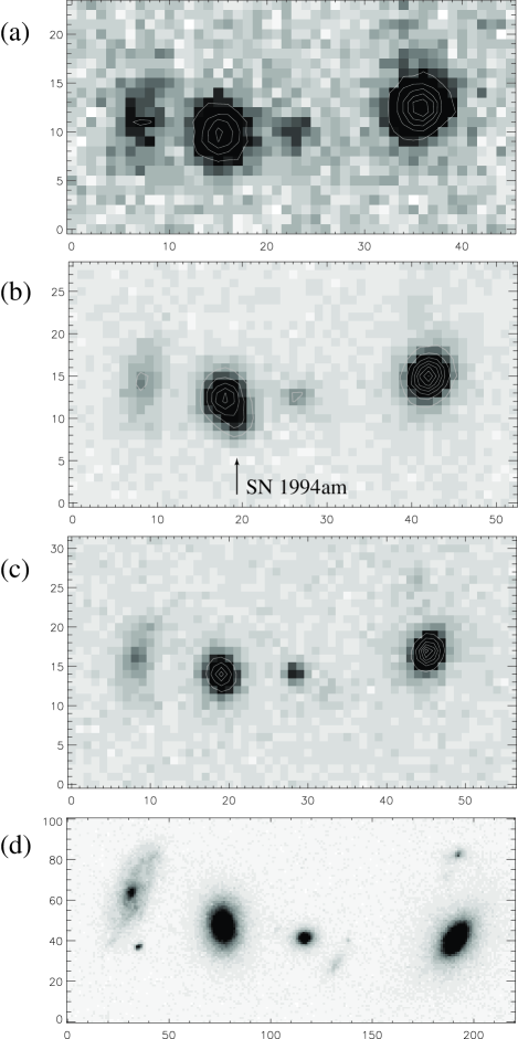
Figure 1: Enlarged subimage showing the host galaxy of SN 1994am, and three neighboring galaxies before, during, and after the supernova explosion. (a) Isaac Newton 2.5-m Harris $R$-band observation on 19 December 1993, with 0.6 arcsec/pixel. (b) Kitt Peak 4-m Harris $R$-band observation on 4 February 1994, with 0.47 arcsec/pixel, near maximum light of the supernova (indicated by arrow). (c) Cerro Tololo 4-m Harris $R$-band observation on 15 October 1995, with 0.47 arcsec/pixel. (d) Hubble Space Telescope (WFPC2) F814W $I$-band observation on 13 January 1995, with 0.1 arcsec/pixel. At this resolution, the host galaxy of SN 1994am can be identified as an elliptical, providing strong evidence that SN 1994am is a type Ia supernova.

Spectra of both SN 1994F and SN 1994G are more consistent with an SN Ia spectrum at the appropriate number of rest-frame days ($t_{\rm spect}$ of Table 1) past the light curve maximum than any alternatives. The spectrum of SN 1994G was observed $\sim$13 days past $B$ maximum (rest frame) at the MMT by P. Challis, A. Riess, and R. Kirshner and $\sim$15 days past maximum at the Keck telescope. The strengths of the Ca II H and K, Fe, and Mg II features closely match those of a SN Ia. The spectrum of SN 1994F was observed $\sim$2 days before maximum (rest frame) by J. B. Oke, J. Cohen, and T. Bida during the commissioning of LRIS at the Keck telescope, and therefore was neither calibrated nor optimally sky-subtracted. The stronger SN I features (e.g. Ca II) do appear to be present nonetheless, so SN 1994F is unlikely to be a luminous SN II near maximum. The spectra for all of these supernovae will be reanalyzed and published once the late-time host-galaxy spectra are available, since host-galaxy features can confuse details of the supernova spectrum.

To address the remaining two unclassified supernovae, we consider the classification statistics of our entire sample of $>$28 supernovae discovered to date by the Supernova Cosmology Project. Eighteen supernovae have been observed spectroscopically, primarily at the Keck 10 m telescope. Of these, the 16 supernovae at redshifts $z\geq 0.35$ discovered by our standard search technique are all consistent with a type Ia identification, while the two closer ($z<0.35$) supernovae are type II. This suggests that $>$94% of the supernovae discovered by this search technique at redshifts $z\geq 0.35$ are type Ia. Moreover, the shapes of the light curves we observe are inconsistent with the “plateau” light curves of SNe IIP, further reducing the probability of a non-type Ia. In this paper, we will therefore assume an SN Ia identification for the remaining two unclassified supernovae.

4.2 Photometry Reduction

The two primary stages of the photometry reduction are the measurement of the supernova flux on each observed point of the light curve, and the fitting of these data to a SN Ia template to obtain peak magnitude and width (stretch factor). At high redshifts, a significant fraction ($\sim$50%) of the light from the supernova’s host galaxy usually lies within the seeing-disk of the supernova, when observed from ground-based telescopes. We subtract this host galaxy light from each photometry point on the light curve. The amount of host galaxy light to be subtracted from a given night’s observation is found from an aperture matched to the size and shape of the point-spread-function for that observation, and measured on the late-time images that are observed after the supernova has faded.

The transmission ratio between the late-time image and each of the other images on the light curve is calculated from the objects neighboring the supernova’s host galaxy that share a similar color (typically $>$25 objects are used). This provides a ratio that is suited to the subtraction of the host galaxy light. Another ratio between the images is calculated for the supernova itself, taking into account the difference between the color of the host galaxy and the color of the supernova at its particular time in the light curve by integrating host-galaxy spectra and template supernova spectra over the filter and detector response functions. (These color corrections were not always necessary since the filter-and-detector response function often matched for different observations.) The magnitudes are thus all referred to the late-time image, for which we observe a series of Landolt (1992) standard fields and globular cluster tertiary standard fields (Christian et al. 1985; L. Davis, private communication). The instrumental color corrections account for the small differences between the instruments used, and between the instruments and the Landolt standard filter curves.

This procedure is checked for each image by similarly subtracting the light in apertures on numerous ($\sim$50) neighboring galaxies of angular size, brightness, and color similar to the host galaxy. If these test apertures, which contain no supernova, show flat light curves then the subtraction is perfect. The RMS deviations from flat test-lightcurves provide an approximate measurement, $\sigma_{\rm test}$, of photometry uncertainties due to the matching procedure together with the expected RMS scatter due to photon noise. We generally reject images for which these matching-plus-photon-noise errors are more than 20% above the estimated photon-noise error alone (see below). (Planned HST light curve measurements will make these steps and checks practically unnecessary, since the HST point-spread-function is quite stable over time, and small enough that the host galaxy will not contribute substantial light to the SN measurement.)

Photometry Point Error Budget. We track the sources of photometric uncertainty at each step of this analysis to construct an error budget for each photometry point of each supernova. The test-lightcurve error, $\sigma_{\rm test}$, then provides a check of almost all of these uncertainties combined. The dominant source of photometry error in this budget is the Poisson fluctuation of sky background light, within the photometry apertures, from the mean-neighborhood-sky level. A typical mean sky level on these images is $N_{\rm sky}=10,000$ photoelectrons (p.e.) per pixel, and it is measured to approximately 2% precision from the neighboring region on the image. Within a 25-pixel aperture, the sky light contributes a Poisson noise of ($25N_{\rm sky})^{1/2}\approx 500$ p.e. The light in the aperture from the supernova itself and its host galaxy is typically $\sim$6,000 p.e., and contributes only $\sim$77 p.e. of noise in quadrature, negligible compared to the sky background noise. Similarly, the noise contribution from the sky light in the subtracted late-time images after the supernova fades is also negligible, since the late time images are typically $\mathrel{\raise 1.1625pt\hbox{$>$}\kern-6.99997pt\lower 3.05696pt\hbox{{$\scriptstyle\sim$}}}$9 times longer exposures then the other images. The supernova photometry points thus typically each have $\sigma_{\rm photon}\approx$ 11% photon-noise measurement error.

Much smaller contributions to the error budget are added by the previously-mentioned calibration and correction steps: The magnitude calibrations have uncertainties between 1% and 4%, and uncertainties from instrumental color corrections are $\leq$1%. Uncertainties introduced in the “flat-fielding” correction for pixel-to-pixel variation in quantum efficiency are less than $1/\sqrt{1}0$ of the sky noise per pixel, since $\mathrel{\raise 1.1625pt\hbox{$>$}\kern-6.99997pt\lower 3.05696pt\hbox{{$\scriptstyle\sim$}}}$10 images are used to calculate the “flat field” for quantum efficiency correction. This flat-fielding error leads to $\sim$32 p.e. uncertainty in the supernova-and-host-galaxy light, which is an additional 5% uncertainty in quadrature above $\sigma_{\rm photon}$. For most images the quadrature sum of all of these error contributions agrees with the overall test dispersion, $\sigma_{\rm test}$. The exceptions mentioned above generally arise from point-spread-function variations over a given image in combination with extremely poor seeing, and such images are generally rejected unless $\sigma_{\rm test}$ is within 20% of the expected quadrature sum of the error contributions.

Since the target fields for the supernova search were chosen at high Galactic latitudes whenever possible, the uncertainties in our Galaxy extinction, $A_{R}$ (based on values of $E(B-V)$ from Burstein & Heiles 1982), are generally $<$1% on the photometry measurement. The one major exception is SN 1994al, for which there is more substantial Galactic extinction, $A_{R}=0.23$ mag, and hence we quote a more conservative extinction error of $\pm$0.11 mag for this supernova.

All of these sources of uncertainties are included in the error budget of Table 1. The photometry data points derived from this first stage of the reduction are shown in Figure 2. Although we observe $\geq$2 images for each night’s data point to correct for cosmic rays and pixel flaws, these images have been combined in producing these plots (and in the preceding noise calculations, for direct comparison). Since the error bars depend on the uncertainty in the host-galaxy measurement, there is significant correlation between them, particularly for nights with similar seeing. Therefore, the usual point-to-point statistics for uncorrelated data do not apply for these plots. Further details concerning the calibration observations, color corrections, and data reduction, with mention of specific nights, telescopes, and supernovae, are given in Perlmutter et al. (1995), and the forthcoming data catalog paper.

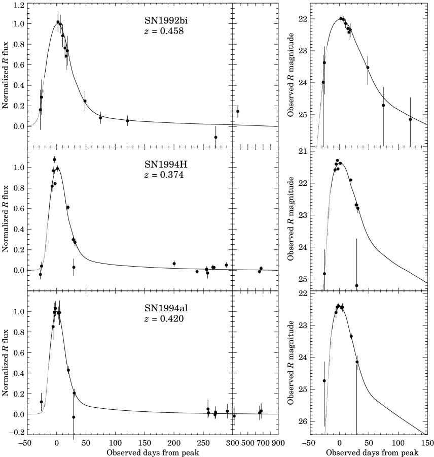
Figure 2: (Continued on next page.) $R$-band light curve photometry points for the first seven high-redshift supernovae discovered by the Supernova Cosmology Project, and best-fit template SN Ia light curves. The left panels show the relative flux as function of observed time (not supernova-rest-frame time). The right panels show observed $R$-band magnitude versus observed time. Note that there is significant correlation between the error bars shown, particularly for observations with similar seeing, since the error bars depend on the uncertainty in the host-galaxy measurement that have been subtracted from these measurements (see text). An $I$-band light curve is also shown for SN 1994G; other photometry points in $I$ and $B$ for the seven supernovae are not shown on this plot. The rising slope (in mag/day) of the template light curve before rest-frame day $-$10 (indicated by the grey part of the curves) is not well-determined, since few low-redshift supernovae are discovered this soon before maximum light. A range of possible rise times was therefore explored (see text).

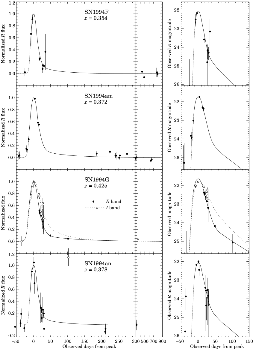
Figure 2: continued.

4.3 Light Curve Fit

At $z\approx 0.4$, the light that leaves the supernova in the $B$ band arrives at our telescopes approximately in the $R$ band. The second stage of the photometry reduction, fitting the light curve, must therefore be performed using a $K$-corrected SN Ia light curve template: We use spectra of several low-redshift supernovae, well-observed over the course of their light curves, to calculate a table of cross-filter $K$ corrections, $K_{BR}(t)$, as a function of light curve time. These corrections account for the mismatch between the redshifted $B$ band and the $R$ band (including the stretch of the transmission-function width), as well as for the difference in the defined zero points of the two magnitude systems. For each high-redshift supernova, we can then construct a predicted $R$-band template light curve as would be observed for the redshift, ${\cal T}_{R}^{\rm observe}$, based on the $B$-band “standard” template (i.e., with $\Delta m_{15}=1.1$ mag) as actually observed in the SN rest frame:

$${\cal T}_{R}^{\rm observe}(t^{\prime})={\cal T}_{B}^{\rm restframe}(t)+K_{BR}(t),$$ (7)

where the observed time dependence, $t^{\prime}\equiv t(1+z)$, accounts for the time dilation of events at redshift $z$. The calculations of $K_{BR}(t)$ are described and tabulated, in Kim, Goobar, & Perlmutter (1996), with an error analysis that yields uncertainties of $<$0.04 mag for redshifts $z<0.6$. Table 1 lists the values of $K_{BR}$ at maximum light for the redshifts of the seven supernovae.

For the exceptional case of SN 1994al, with significant $E(B$$-$$V)$ from our own Galaxy, we also calculate the extinction, $A_{R}$, as a function of supernova-rest-frame time, again using a series of redshifted supernova spectra multiplied by a reddening curve for an $E(B$$-$$V)_{\rm B\&H}$ value given by Burstein & Heiles (1982). For this particular supernova’s redshift, $A_{R}=0.23\pm 0.11$, with variations of 0.01 magnitude for the dates observed on the light curve. For the redshifts of all seven supernovae, we find essentially the same ratio ${\cal R}_{R}=A_{R}/E(B$$-$$V)_{\rm B\&H}=2.58\pm 0.01$, at maximum light.

The photometry data points for each supernova are fit to the as-observed $R$-band template, ${\cal T}_{R}^{\rm observe}$, with free parameters for the stretch-factor, $s$, the $R$ magnitude at peak, $m_{R}$, the date of peak, $t_{\rm peak}$, and the additive constant flux, $g_{\rm resid}$, that accounts for the residual host-galaxy light due to Poisson error in the late-time image:

$$f(t;m_{R},s,t_{\rm peak},g_{\rm resid})=10^{-0.4\left[m_{R}-m_{R}^{\rm 0}+{\cal T}_{R}^{\rm observe}(t^{\prime}s-t_{\rm peak})\right]}+g_{\rm resid}\;,$$ (8)

where $m_{R}^{\rm 0}$ is the calibration zero-point for the $R$ observations and ${\cal T}_{R}^{\rm observe}(t)$ is normalized to zero at $t=0$. (For one of the supernovae with sufficient $I$ band data, SN 1994G, the fitting function $f$ also includes the redshifted, $K$-corrected $V$-band template, and an additional parameter for the $R$$-$$I$ color at maximum is fit.) We fit to flux measurements, rather than magnitudes, because the error bars are symmetric in flux, and because the data points have the late-time galaxy light subtracted out and hence can be negative. In this fit, particular care is taken in constructing the covariance matrix (see, e.g., Barnett et al. 1996) to account for the correlated photometry error due to the fact that the same late-time images of the host galaxy are used for all points on a light curve.

Light Curve Error Budget. We compute uncertainties for $m_{R}$ and $s$ using both a Monte Carlo study and a mapping of the $\chi^{2}$ function; both methods yield similar results. Table 1 lists the best-fit values and uncertainties for $m_{R}$ and $s$. Usually, many data points contribute to the template fit, so the uncertainty in the peak, $m_{R}$, is less than the typical $\sim$11% photometry uncertainty in each individual point. However, our Monte Carlo studies show that it is usually very important that high quality late-time and pre-maximum data points be available to constrain both $s$ and $m_{R}$. We have explored the consequences of adding or subtracting observations on the light curves, although the error bars reflect the actual light curve sampling observed for a given supernova.

The rising slope of the template light curve before rest-frame day $-$10 (indicated by the grey part of the curves in Figure 2) is not well-determined, since few low-redshift supernovae are discovered this soon before maximum light. A range of possible rise times was therefore also explored. Only two of the supernovae show any sensitivity to the choice of rise time. The effect is well within the error bars of the stretch factor, and negligible for the other parameters of the fit.

For the analyses of this paper, we translate these observed $R$ magnitudes back to the “effective” $B$ magnitudes, $m_{B}=m_{R}-A_{R}-K_{BR}$, where all the quantities (see Table 1) are for the light curve $B$-band peak (SN rest frame), and we have corrected for Galactic extinction, $A_{R}$, at this stage. In the following section, we directly compare these “effective” $B$ magnitudes with the $B$ magnitudes of the low-redshift supernovae using the equations of Section 2, substituting the $K$-corrected effective $B$ magnitudes, $m_{B}$, and the $B$-band zero point, ${\cal M}_{B}$, for the bolometric magnitudes, $m$ and ${\cal M}$.

5 Results for the High-Redshift Supernovae

5.1 Dispersion and Width-Brightness Relation

Before using a width-luminosity correction, it is important to test that it applies at high redshifts, and that the magnitude dispersions with and without this correction are consistent with those of the low-redshift supernovae. We study the peak-magnitude dispersion of the seven high-redshift supernovae by calculating their absolute magnitudes for an arbitrary choice of cosmology. This allows the relative magnitudes of the supernovae at somewhat different redshifts ($z=0.35$–0.46) to be compared. The slight dependence on the choice of cosmology is negligible for this purpose, for a wide range of $\Omega_{\rm M}$ and $\Omega_{\Lambda}$. Choosing $\Omega_{\rm M}=1$ and $\Omega_{\Lambda}=0$, the RMS dispersion about the mean absolute magnitude for the seven supernovae is $\sigma_{M_{B}}=0.27$. (We find the same RMS dispersion for the best-fit cosmology discussed below in Section 5.3.)

Figure 3 shows the difference between the measured and the “theoretical” (Equation 4 for $\Omega_{\rm M}=1$, $\Omega_{\Lambda}=0$ and ${\cal M}={\cal M}_{B,{\rm corr}}^{\scriptscriptstyle\{1.1\}}$) uncorrected effective $B$ magnitudes, $m_{B}-m_{B}^{\rm theory}$, as a function of the best-fit stretch factor $s$ or, equivalently, $\Delta m_{15}$. The zero-point intercept, ${\cal M}_{B,{\rm corr}}^{\scriptscriptstyle\{1.1\}}$, from Equation 5 was used in the calculation of $m_{B}^{\rm theory}$, so that the data points could be compared to the Equation 5 width-luminosity relation found for the nearby sample of Hamuy et al. (the solid line of Figure 3). A different choice of ($\Omega_{\rm M}$, $\Omega_{\Lambda}$) or of the magnitude zero-point ${\cal M}$ would move the line in the vertical direction relative to the points, so the comparison should be made with the shape of the relation, not the exact fit. The width-luminosity relation seen for nearby supernovae appears qualitatively to hold for the high-redshift supernovae.

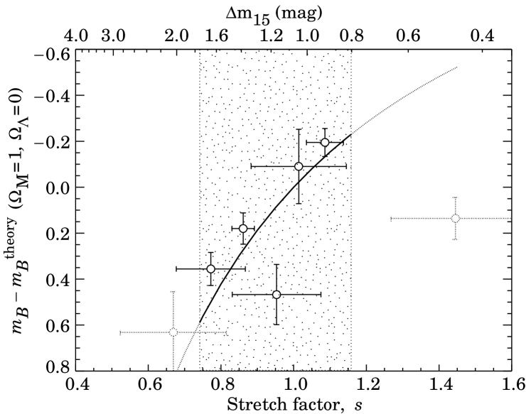
Figure 3: The difference between the measured and “theoretical” (Equation 4 for $\Omega_{\rm M}=1$, $\Omega_{\Lambda}=0$, and ${\cal M}={\cal M}_{B,{\rm corr}}^{\scriptscriptstyle\{1.1\}}$) $B$ magnitudes (uncorrected for the width-luminosity relation) versus the best-fit stretch factor, $s$, for the high-redshift supernovae. The stretch factor is fit in the supernova rest frame, i.e., after correcting for the cosmological time dilation calculated from the host-galaxy redshift (see Equations 7 and 8). If different values of ($\Omega_{\rm M}$, $\Omega_{\Lambda}$) had been chosen the labels would change, but the data points would not vary significantly within their error bars, since the range of redshifts is not large for these supernovae. The upper axis gives the equivalent values of $\Delta m_{15}=1.96(s^{-1}-1)+1.07$ (Eq. 6). The solid line shows the width-luminosity relation (Eq. 5) found by Hamuy et al. (1995, 1996) for an independent set of 18 nearby ($z\leq 0.1$) SNe Ia, for which $0.8\mathrel{\raise 1.1625pt\hbox{$<$}\kern-6.99997pt\lower 3.05696pt\hbox{{$\scriptstyle\sim$}}}\Delta m_{15}\mathrel{\raise 1.1625pt\hbox{$<$}\kern-6.99997pt\lower 3.05696pt\hbox{{$\scriptstyle\sim$}}}1.75$ mag. This range of light-curve widths is indicated by the shaded region. The curve and data points outside of this range are plotted in a different shade to emphasize that the relation is only established within this range. A different choice of ($\Omega_{\rm M}$, $\Omega_{\Lambda}$) or of the magnitude zero-point ${\cal M}$ would move the line in the vertical direction relative to the points.

To make this result quantitative, we use the prescription of Equation 5 to “correct” the magnitudes to that of a supernova with $\Delta m_{15}=1.1$ mag, by adding magnitude corrections, $\Delta_{\rm corr}^{\scriptscriptstyle\{1.1\}}=-0.86(\Delta m_{15}-1.1)$, where we derive $\Delta m_{15}$ from $s$ using Equation 6. Note that the resulting corrected magnitude, $m_{B,{\rm corr}}=m_{B}+\Delta_{\rm corr}^{\scriptscriptstyle\{1.1\}}$, listed in Table 1, has an uncertainty that is not necessarily the quadratic sum of the uncertainties for $m_{B}$ and $\Delta_{\rm corr}^{\scriptscriptstyle\{1.1\}}$, because the best-fit values for $s$ and $m_{R}$ (and hence $m_{B}$) are correlated in the light-curve template fit.

Two of the high-redshift supernovae (shown with different-shaded symbols in Figure 3 and subsequent figures) have values of $\Delta m_{15}$ that are outside of the range of values studied in the low-redshift supernova data set of Hamuy et al. The width-luminosity correction for these supernovae is therefore less reliable than for the other five supernovae, since it depends on an extrapolation. It is also possible that the true values of $\Delta m_{15}$ for the two supernovae fall within this range, given the fit error bars. (One of these, SN 1992bi at $z=0.458$, has very large error bars because its light curve has larger photometric uncertainties and the lightcurve sampling was not optimal to constrain the stretch factor $s$.) In Table 1, the corrections, $\Delta_{\rm corr}^{\scriptscriptstyle\{1.1\}}$, and corrected magnitudes, $m_{B,{\rm corr}}$, for these supernovae are therefore listed in brackets, and we also give the corrected magnitudes, $m_{B,{\rm corr}}^{\rm extreme}$, obtained using only the most extreme $\Delta_{\rm corr}^{\scriptscriptstyle\{1.1\}}$ corrections found for low-redshift supernovae. In the following analysis we calculate all results using just the other five supernovae that are within the Hamuy et al. range of $\Delta m_{15}$. As a cross-check, we then provide the result using all seven supernovae, but without width-luminosity correction.

The peak-magnitude RMS dispersion for the five high-redshift supernovae that are within the $\Delta m_{15}$ range improves from $\sigma_{M_{B}}=0.25$ mag before applying the width-luminosity correction to $\sigma_{M_{B},{\rm corr}}=0.19$ mag after applying the correction. These values agree with those for the 18 low-redshift Calán/Tololo supernovae, $\sigma_{M_{B}}^{\rm Hamuy}=0.26$ and $\sigma_{M_{B},{\rm corr}}^{\rm Hamuy}=0.17$ mag, suggesting that the supernovae at high-redshift are drawn from a similar population, with a similar width-luminosity correlation. Note that although the slope of the width-luminosity relation, Equation 5, stays the same, it is possible that the intercept could change at high redshift, but this would be a remarkable conspiracy of physical effects, since the time scale of the event appears naturally correlated with the strength and temperature of the explosion (see Nugent et al. 1996).

5.2 Color and Spectral Indicators of Intrinsic Brightness

With the supplementary color information in the $I$ and $B$ bands, and the spectral information for three of the supernovae, we can also begin to test the other indicators of intrinsic brightness within the SN Ia family. The broadest, most luminous supernova of our five-supernova subsample, SN 1994H, is bluer than $B$$-$$R=0.7$ at the 95% confidence level $2\pm 2$ days before maximum light (this is only a limit because of possible clouds on the night of the $B$ calibration). For comparison, Nugent (1996, private communication) has estimated observed $B$$-$$R$ colors within $\sim$4 days of maximum light as a function of redshift using spectra for a range of SN Ia sub-types, from the broad, superluminous SN 1991T to the narrow, subluminous SN 1991bg. SN 1994H is only slightly bluer than the $B$$-$$R\approx 1.0\pm 0.15$ color of SN 1991T at $z=0.374$ (where the error represents the range of possible host-galaxy reddening). However, SN 1994H does not agree with the redder colors (at $z=0.374$) of SN 1981B ($B$$-$$R\approx 1.7$ mag) and SN 1991bg ($B$$-$$R\approx 2.6$ mag). SN1991T has a broad light curve width of $\Delta m_{15}=0.94\pm 0.07$, which agrees within error with the light curve width of SN 1994H, $\Delta m_{15}=0.91\pm 0.09$, whereas SN 1981B and SN 1991bg both have “normal” or narrower light curve widths, $\Delta m_{15}=1.10\pm 0.07$ and $\Delta m_{15}=1.93\pm 0.10$ mag.

The multi-band version of the “correction template” analysis (Riess et al. 1996) is designed to fit simultaneously for the host galaxy extinction (discussed later) and the intrinsic brightness of the supernova. The rest frame $V$ light curve (approximately redshifted into our observed $I$) is the strongest indicator of the SN Ia family parameterization when using this approach. We thus use this technique to analyze SN1994G, with its well sampled $I$ light curve in addition to $R$ data. We find that the supernova is best fit by a correction template that indicates that it is intrinsically overluminous by $0.06\pm 0.38$ magnitudes, compared to a Leibundgut-template supernova. This is consistent with the $0.05\pm 0.22$ overluminosity found using the width-luminosity correlation and the best-fit stretch factor.

(The “correction template” fit gives larger error bars than a simple stretch-factor fit because the correction templates have significant uncertainties, with day-to-day correlations that are, unfortunately, not tabulated. Currently, the fits to $B$-band correction templates have even larger uncertainties than $V$-band, possibly due to a poor fit of the linear correction model to the low-redshift data. This approach is therefore not useful for the other six high-redshift supernovae of this first set, since these large correction-template uncertainties propagate into $>$1 magnitude uncertainties in the fits to the observed $R$ band data.)

Both intrinsically fainter supernovae and supernovae with host galaxy extinction can appear redder in $R$$-$$I$ (corresponding to approximately $B$$-$$V$ in the supernova rest frame). For the several supernova for which we have scattered $I$-band photometry, we thus can use it to estimate extinction only after the supernova sub-type has been determined using the stretch factor. SN 1994G fit closely to the $s=1$ template. An $s=1$ supernova at $z=0.420$ will have an expected observed color $R-I=0.16\pm 0.05$ mag at observed-$R$ maximum light. For SN 1994G, we observed $R-I=-0.12\pm 0.17$ mag. This gives $E(R$$-$$I)_{\rm observed}\approx E(B-V)_{\rm restframe}=-0.28\pm 0.18$ mag, or $A_{V}<0.01$ mag at the 95% confidence level. The Riess et al. “correction template” analysis of SN 1994G also yields a bound on extinction of $A_{V}<0.01$ mag (90% confidence).

The more recent high-redshift supernovae studied by the Supernovae Cosmology Project have more complete color and spectral data, and so should soon provide further tests of these additional SN Ia luminosity indicators. In addition, the spectrum of SN 1994an covers both wavelength regions in which the Nugent et al. (1996) line ratios correlate well with supernova magnitudes. This analysis awaits the availability of the spectrum of the host galaxy without the supernova light, so that we can subtract the galaxy-spectrum “contamination” from the supernova spectrum. Further late-time $B$-band images of SN 1994an will also allow $B$$-$$R$ color cross-checks using $B$ images that were observed four days after maximum.

5.3 Magnitude-Redshift Relation and the Cosmological Parameters

Figure 4(a) shows the Hubble diagram, $m_{B}$ versus $\log cz$, for the seven high-redshift supernovae, along with low-redshift supernovae of Hamuy et al. (1995) for visual comparison. The solid curves are plots of $m_{B}^{\rm theory}$, i.e., Equation 4 with ${\cal M}={\cal M}_{B}$ for three $\Lambda=0$ cosmologies, ($\Omega_{\rm M}$, $\Omega_{\Lambda}$) = (0, 0), (1, 0), and (2, 0); the dotted curves, which are practically indistinguishable from the solid curves, are for three flat cosmologies, ($\Omega_{\rm M}$, $\Omega_{\Lambda}$) = (0.5, 0.5), (1, 0), and (1.5, $-$0.5). These curves show that the redshift range of the present supernova sample begins to distinguish the values of the cosmological parameters. Figure 4(b) shows the same magnitude-redshift relation for the data after adding the width-luminosity correction term, $\Delta_{\rm corr}^{\scriptscriptstyle\{1.1\}}$; the curves of $m_{B}^{\rm theory}$ in (b) are calculated for ${\cal M}={\cal M}_{B,{\rm corr}}^{\scriptscriptstyle\{1.1\}}$.

Figure 5 shows the 68% (1$\sigma$), 90%, and 95% (2$\sigma$) confidence regions on the $\Omega_{\rm M}$–$\Omega_{\Lambda}$ plane for the fit of Equation 4 to the high-redshift supernova magnitudes, $m_{B,{\rm corr}}$, after width-luminosity correction, using ${\cal M}={\cal M}_{B,{\rm corr}}^{\scriptscriptstyle\{1.1\}}$. In this fit, the magnitude dispersion, $\sigma_{M_{B},{\rm corr}}^{\rm Hamuy}=0.17$, is added in quadrature to the error bars of $m_{B,{\rm corr}}$ to account for the residual intrinsic dispersion, after width-correction, of our model (low-redshift) standard candles.

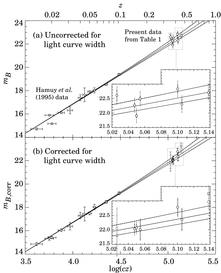
Figure 4: Hubble diagrams for the first seven high-redshift supernovae, (a) uncorrected $m_{B}$, with low-redshift supernovae of Hamuy et al. (1995) for visual comparison; (b) $m_{B,{\rm corr}}$ after “correction” for width-luminosity relation. The square points are not used in the analysis, because they are corrected based on an extrapolation outside the range of light curve widths of low-redshift supernovae (see text and Table 1). Insets show the high-redshift supernovae on magnified scales. The solid curves in (a) and (b) are theoretical $m_{B}$ for ($\Omega_{\rm M}$, $\Omega_{\Lambda}$) = (0, 0) on top, (1, 0) in middle, and (2, 0) on bottom. The dotted curves, which are practically indistinguishable from the solid curves, are for the flat universe case, with ($\Omega_{\rm M}$, $\Omega_{\Lambda}$) = (0.5, 0.5) on top, (1, 0) in middle, and (1.5, $-$0.5) on bottom. The inner error bars on the data points show the photometry measurement uncertainty, while the outer error bars add the intrinsic dispersions found for low-redshift supernovae, $\sigma_{M_{B}}^{\rm Hamuy}$ for (a) and $\sigma_{M_{B},{\rm corr}}^{\rm Hamuy}$ for (b), for comparison to the theoretical curves. Note that the zero-point magnitude used for (b), ${\cal M}_{B,{\rm corr}}^{\scriptscriptstyle\{1.1\}}$, and hence the effective $m_{B}$ scale, is shifted slightly from the uncorrected ${\cal M}_{B}$ used for the curves of (a).

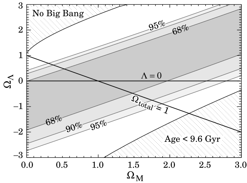
Figure 5: Contour plot of the 68% (1$\sigma$), 90%, and 95% (2$\sigma$) confidence regions in the $\Omega_{\Lambda}$ versus $\Omega_{\rm M}$ plane, for the first seven high-redshift supernovae. The solid lines show the two special cases of a $\Lambda=0$ cosmology and a flat ($\Omega_{\rm total}\equiv\Omega_{\rm M}+\Omega_{\Lambda}=1$) cosmology. (Note that the constrained one-dimensional confidence intervals for $\Lambda=0$ or $\Omega_{\rm total}=1$ are smaller than the intersection of these lines with the two-dimensional contours, as discussed in the text.) The two labeled corners of the plot are ruled out because they imply: (upper left corner) a “bouncing” universe with no big bang (see Carroll et al. 1992), or (lower right corner) a universe younger than the oldest heavy elements, $t_{0}<9.6$ Gyr (Schramm 1990), for any value of $H_{0}\geq 50$ km s^-1 Mpc^-1.

The two special cases represented by the solid lines of Figure 5 yield significant measurements: We again fit Equation 4 to the high-redshift supernova magnitudes, $m_{B,{\rm corr}}$, but this time with the fit constrained first to a $\Lambda=0$ cosmology (the horizontal line of Figure 5), and then to a flat universe (the diagonal line of Figure 5, with $\Omega_{\rm total}\equiv\Omega_{\rm M}+\Omega_{\Lambda}=1$). In the case of a $\Lambda=0$ cosmology, we find the mass density of the universe to be $\Omega_{\rm M}=0.88\;^{+0.69}_{-0.60}$. For a flat universe (the diagonal line of Figure 5, with $\Omega_{\rm total}\equiv\Omega_{\rm M}+\Omega_{\Lambda}=1$), we find the cosmological constant to be $\Omega_{\Lambda}=0.06\;^{+0.28}_{-0.34}$, consistent with no cosmological constant. For comparison with other results in the literature, we can also express this fit as a 95% confidence level upper limit of $\Omega_{\Lambda}<0.51$. Finally, this fit can be described by the value of the mass density, $\Omega_{\rm M}=1-\Omega_{\Lambda}=0.94\;^{+0.34}_{-0.28}$. (For brevity, we will henceforth only quote the $\Omega_{\Lambda}$ fit results for the flat-universe case, since either $\Omega_{\Lambda}$ or $\Omega_{\rm M}$ can be used to parameterize the flat-universe fit.) The goodness-of-fit is quantified by $Q(\chi^{2}|\nu)$, the probability of obtaining the best-fit $\chi^{2}$ or higher for $\nu=N_{\rm SNe}-1$ degrees of freedom (following the notation of Press et al. 1986, p. 165). For both the $\Lambda=0$ and flat universe cases, $Q(\chi^{2}|\nu)=0.75$.

The error bars on the measurement of $\Omega_{\Lambda}$ or $\Omega_{\rm M}$ for a flat universe are about two times smaller than the error bars on $\Omega_{\rm M}$ for a $\Lambda=0$ universe. This can be seen graphically in Figure 5, in which the confidence region strip makes a shallow angle with respect to the $\Omega_{\Lambda}=0$ line but crosses the $\Omega_{\rm total}=1$ line at a sharper angle. Note that these error bars in the constrained one-dimensional fits for $\Lambda=0$ or $\Omega_{\rm total}=1$ are smaller than the intersection of the constraint lines of Figure 5 and the 68% contour band. This is because a different range of $\Delta\chi^{2}\equiv\chi^{2}-\chi^{2}_{\rm min}$ corresponds to 68% confidence for one free parameter, $\nu=1$ degree of freedom, as opposed to two free parameters, $\nu=2$ (see Press et al. 1986, pp. 532-7).

We also analyzed the data for the same five supernovae “as measured,” that is, without correcting for the width-luminosity relation, and taking the uncorrected zero point, ${\cal M}_{B}=-3.17\pm 0.03$ of Hamuy et al. (1996). We find essentially the same results: $\Omega_{\rm M}=0.93\;^{+0.69}_{-0.60}$ for $\Lambda=0$ and $\Omega_{\Lambda}=0.03\;^{+0.29}_{-0.34}$ for a flat $\Omega_{\rm total}=1$ universe. The measurement uncertainty for the analysis using light-curve-width correction is not significantly better than this one, without correction, because for this particular data set the smaller calibrated dispersion, $\sigma_{M_{B},{\rm corr}}$ as opposed to $\sigma_{M_{B}}$, is offset by the uncertainties in the measurements of the light curve widths. The goodness of fit, however, for the uncorrected magnitudes is lower, $Q(\chi^{2}|\nu)=0.34$, for both the $\Lambda=0$ and flat universe. This indicates that the width-luminosity relation provides a better model, although this was already seen in the improved RMS dispersion of the corrected magnitudes. Table 2 summarizes the results.

As a cross-check, we also analyzed the results for all seven supernovae, not “width-corrected,” including the two that had measured widths outside the range of the low-redshift width correction. We find $\Omega_{\rm M}=0.70\;^{+0.57}_{-0.49}$ for $\Lambda=0$ and $\Omega_{\Lambda}=0.15\;^{+0.24}_{-0.28}$ for $\Omega_{\rm total}=1$.

We emphasized in Section 2 that the 1$\sigma$ confidence region of Figure 5 is not parallel to the contours of constant $q_{0}$. For comparison, the $q_{0}$ contours are drawn (dashed lines) in Figure 6. The closest $q_{0}$ contour varies from $\sim$0.5 to $\sim$1 in the region with $\Omega_{\rm M}\leq 1$. Any single value of $q_{0}$ would thus be only a rough approximation to the true confidence interval dependent on $\Omega_{\rm M}$ and $\Omega_{\Lambda}$ shown in Figure 6.

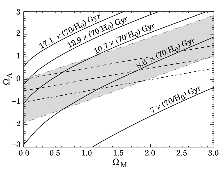
Figure 6: Contour plot of the 1$\sigma$ (68%) confidence region in the $\Omega_{\Lambda}$ versus $\Omega_{\rm M}$ plane, for the first seven high-redshift supernovae. The solid lines show contours for the age of the universe (in Gyr), normalized to $H_{0}=70$ in units of km s^-1 Mpc^-1. The dashed lines are the contours of constant deceleration parameter $q_{0}$ = 0.0 (top), 0.5 (middle), 1.0 (bottom).

6 Checks for Sources of Systematic Error

Since this is a first measurement of cosmological parameters using SNe Ia, we list here some of the more important concerns, together with the checks and tests that would address them. By considering each of the separate subsamples of SNe that avoid a particular source of bias, we can show that no one source of systematic error alone can be responsible for the measured values of $\Omega_{\rm M}$ and $\Omega_{\Lambda}$. We cannot, however, exclude a conspiracy of biases each moving an individual supernova’s measured values into agreement with this result. Fortunately, this sample of seven supernovae is only the beginning of a much larger data set of SNe Ia at high redshifts, with more complete multiband light curves and spectral coverage.

Width-Brightness Correction. For the present data set, the measurements of $\Omega_{\rm M}$ and $\Omega_{\Lambda}$ are the same whether or not we apply the light-curve width-luminosity correction, and so do not depend upon our confidence in this empirical calibration. This is due to the similar distribution of light curve widths for the high-redshift supernovae and the low-redshift supernovae used for calibration.

For future data sets, it is possible that the width distribution will differ, for example if we were to find more supernovae in clusters of ellipticals and confirm the tendency to find narrower/fainter supernovae in ellipticals. (Note that SN 1994am, in an elliptical host, does in fact have a somewhat narrow light curve, with $s=0.84$.) For such a data set the result would depend on the validity of the width-luminosity correction. Such a correction dependence could be checked by restricting the analysis to the supernovae that pass the Vaughan et al. (1995) $B$$-$$V$ color test for “normals,” and then applying no width-luminosity correction.

Extinction. While the extinction due to our own Galaxy has been incorporated in this analysis, we do not know the SN host-galaxy extinctions. Note that correcting for any neglected extinction for the high-redshift supernovae would tend to brighten our estimated SN effective magnitudes and hence move the best fit of Equation 4 towards even higher $\Omega_{\rm M}$ and lower $\Omega_{\Lambda}$ than the current results. We can check that the extinction is not strongly affecting the results by considering two supernovae for which there is evidence against significant extinction. SN 1994am is in an elliptical galaxy, and for SN 1994G there is the previously-mentioned $R$$-$$I$ color that provides evidence against significant reddening. The best fit values for this two-SN subset are consistent with that of the full set of SNe: $\Omega_{\rm M}=1.31\;^{+1.23}_{-0.98}$ for $\Lambda=0$ and $\Omega_{\Lambda}=-0.15\;^{+0.47}_{-0.61}$ for $\Omega_{\rm total}=1$.

If there were uncorrected host-galaxy extinction for the low-redshift supernovae used to find the magnitude zero point ${\cal M}$, this would lead to an opposite bias. The 18 Calán/Tololo supernovae, however, all have unreddened colors ($B-V<0.2$ mag). For the range of widths of these supernovae ($0.8\mathrel{\raise 1.1625pt\hbox{$<$}\kern-6.99997pt\lower 3.05696pt\hbox{{$\scriptstyle\sim$}}}\Delta m_{15}\mathrel{\raise 1.1625pt\hbox{$<$}\kern-6.99997pt\lower 3.05696pt\hbox{{$\scriptstyle\sim$}}}1.75$ mag), the range of intrinsic color at maximum light should be $-0.05\mathrel{\raise 1.1625pt\hbox{$<$}\kern-6.99997pt\lower 3.05696pt\hbox{{$\scriptstyle\sim$}}}B-V\mathrel{\raise 1.1625pt\hbox{$<$}\kern-6.99997pt\lower 3.05696pt\hbox{{$\scriptstyle\sim$}}}0.5$ mag, so the color excess is limited to $E(B-V)<0.25$ mag. A stronger constraint can be stated for the seven of these 18 Calán/Tololo supernovae that were included in a sample studied by Riess et al. (1996), who used the multicolor correction-template method to estimate extinction. They found that only one of these seven supernovae showed any significant extinction. (For that one supernova, SN 1992P, they found $A_{V}=0.11$ mag.) It is thus unlikely that host-galaxy extinction of the Calán/Tololo supernovae is strongly biasing our results, although it will be useful to test the remaining supernovae of this set for evidence of extinction, using the multicolor correction-template method. (It should be noted that the method of Riess et al. estimates total extinction values for several supernovae that are significantly less than the Galactic extinction estimated by Burstein & Heiles 1982, hence some caution is still necessary in interpreting these results.)

A general argument can be made even without these color measurements: the intrinsic magnitude dispersions, $\sigma_{M_{B},{\rm corr}}^{\rm Hamuy}=0.17$ or our value $\sigma_{M_{B},{\rm corr}}=0.19$ mag, provide an upper bound on the typical extinction present in either the low redshift or the high redshift supernova samples, since a broad range of host-galaxy extinction (which would have a larger mean extinction) would inflate these dispersions. We use Monte Carlo studies to bound the amount of bias due to a distribution of extinction that would inflate a hypothetical intrinsic dispersion of $\sigma_{M_{B}}^{\rm hypothesis}=0.13$ to the values actually measured, $\sigma_{M_{B},{\rm corr}}^{\rm Hamuy}=0.17\pm 0.04$ and $\sigma_{M_{B},{\rm corr}}=0.19\pm 0.08$ mag. We find, at the 90% confidence level, less than 0.06 magnitude bias towards higher $\Omega_{\rm M}$ and lower $\Omega_{\Lambda}$ and less than 0.10 magnitude bias towards lower $\Omega_{\rm M}$ and higher $\Omega_{\Lambda}$. These measurements and bounds on extinction will be even more important as we study supernovae at still higher redshifts and need to check for evolution in the host galaxy dust.

We choose high Galactic latitude fields whenever possible, so that the extinction correction for our own Galaxy and its uncertainty are negligible. The one major exception in this current data set is SN 1994al, with $A_{R}\approx 0.23$ mag. (This supernova also appears to be a somewhat fainter outlier among the width-corrected magnitudes on Figure 4b.) Since there is more uncertainty in the Galactic extinction correction for this supernova, we have fit just the other four width-corrected supernova magnitudes. For SN 1994H, SN 1994am, SN 1994G, and SN 1994an, we find $\Omega_{\rm M}=1.25\;^{+0.82}_{-0.69}$ for $\Lambda=0$ and $\Omega_{\Lambda}=-0.12\;^{+0.33}_{-0.40}$ for $\Omega_{\rm total}=1$.

K Correction. The generalized $K$ correction used to transform $R$-band magnitudes of high redshift SNe to $B$-band rest frame magnitudes was tested for a variety of SN Ia spectra and found to vary by less than 0.04 mag for redshifts $z<0.6$ (Kim, Goobar, & Perlmutter 1996). The test spectra sample included examples in the range of light-curve widths between $\Delta m_{15}=0.94$ mag (for SN 1991T) and $\Delta m_{15}=1.47$ mag (for SN 1992A), but $K$ corrections still need to be calculated to check for possible difference outside of this regime of the SN Ia family. Two of the five supernovae we used in our measurement fall just outside of this range of widths. As a check of a possible systematic error due to this, we consider just the subsample of three supernovae, SN 1994al, SN 1994am, and SN 1994G, with light curve widths within the studied range of $K$ corrections. We find $\Omega_{\rm M}=0.61\;^{+0.89}_{-0.61}$ for $\Lambda=0$ and $\Omega_{\Lambda}=0.18\;^{+0.35}_{-0.43}$ for $\Omega_{\rm total}=1$.

Malmquist Bias. The tendency to find the most luminous members of a distribution at large distances in a magnitude-limited search would appear to bias our results towards larger values of $\Omega_{\rm M}$ and lower values of $\Omega_{\Lambda}$. However, as the SN Ia Hubble diagram uses the peak brightness rather than that at detection, and the supernovae are “corrected” from different intrinsic brightnesses, any such Malmquist bias would not operate the same way it does for a population of normally-distributed static standard candles. The key issue is whether supernova samples are strongly biased at the detection level, as would be the case if most supernovae were discovered close to the threshold value. Our detection-efficiency studies (see Pain et al. 1996) show that the seven high-redshift supernovae were detected approximately 0.5 to 2 magnitudes brighter than our limiting (50% efficiency) detection magnitude, $m_{{}_{d{-}50}}$ (see the final row of Table 1), and the efficiency on our CCD images drops off slowly beyond this limit. (Several of the SNe that we find at a significantly brighter magnitude than our threshold are in clusters that are closer than the limiting distance for a SN Ia. Such inhomogeneities in galaxy distribution can lead to a sample of supernovae that are not distributed primarily near the magnitude limit as expected in a magnitude limited search.) In contrast, the Calán/Tololo survey detected most of the low-redshift supernovae within $\sim$0.7 magnitude of detection threshold and their efficiency on photographic plates dropped quickly beyond that limit (Maza, private communication). Malmquist bias may therefore result, counter-intuitively, in a slightly more luminous sample of the intrinsic SN Ia distribution for the low-redshift photographic search than for the high-redshift CCD search.

Since, however, our current results already suggest a relatively high value for $\Omega_{\rm M}$ and low value for $\Omega_{\Lambda}$, we have nonetheless checked the possibility of Malmquist bias distorting the distributions of magnitudes we find at high redshift. First, as a rough test, we have compared the results (uncorrected for light-curve width) for the three supernovae discovered closest to the 50%-efficiency detection threshold, $m_{{}_{d-50}}$, to the three supernovae discovered farthest from the threshold. We find that the difference in measured $\Omega_{\rm M}$ and $\Omega_{\Lambda}$ between these two subsets is not significant, and it is opposite to the direction of Malmquist bias.

A more detailed quantitative study was based on a Monte Carlo analysis, in which the detection efficiency curve for each supernova was used with the Calán/Tololo “corrected” magnitude dispersion, $\sigma_{{M}_{B},{\rm corr}}^{\rm Hamuy}$, to estimate the magnitude bias that should be present for each of the seven fields on which we discovered high-redshift supernovae. We find that only one supernova, SN 1994G, is on a field that shows any significant magnitude bias. Even for this supernova the bias, 0.01 mag, is still well below the intrinsic dispersion of the supernovae. Hence, when we reanalyze the data set, correcting SN 1994G by this amount, we find an insignificant change in our results for $\Omega_{\rm M}$ and $\Omega_{\Lambda}$.

Because the high-redshift supernovae include both intrinsically narrow, subluminous cases and intrinsically broad, overluminous cases at comparable redshifts, a simple cross-check for Malmquist bias that is independent of detection-efficiency studies can be made by comparing the results for these two subsets separately. Malmquist bias would affect these two subsets differently, leading to a higher $\Omega_{\rm M}$ and lower $\Omega_{\Lambda}$ for the broad, overluminous subsample than for the narrow, subluminous subsample. With our current sample we can compare only two supernovae in each of these subsamples that are in the “correctable” range of $\Delta m_{15}$, so this will be a particularly interesting test to apply to the full sample of high-redshift supernovae when their light-curve observations are completed. The current data show no evidence of Malmquist bias.

Supernova Evolution. Although there are theoretical reasons to believe that the physics of the supernova explosion should not depend strongly on the evolution of the progenitor and its environment, the empirical data are the final arbiters. Both the low-redshift and high-redshift supernovae are discovered in a variety of host galaxy types, with a range of histories. The small dispersion in intrinsic magnitude across this range, particularly after the width-luminosity correction, is itself an indication that any evolution is not changing the relationship between the light curve width/shape and its absolute brightness. (Note that the one supernova in an identified elliptical galaxy gives results for the cosmological parameters consistent with the full sample of supernovae; such a comparative test will of course be more useful with the larger samples.) In the near future, we will be able to look directly for signs of evolution in the $>$18 spectra observed for the larger sample of high-redshift supernovae. So far, the spectral features studied match the low-redshift supernova spectra for the appropriate day on the light curve (in the supernova rest frame), showing no evidence for evolution. A more detailed analysis will soon be possible, as the host galaxy spectra are observed after the supernovae fade, and it becomes possible to study the supernova spectra without galaxy contamination.

Gravitational Lensing. Since the mass of the universe is not homogeneously distributed, there is a potential source of increased magnitude dispersion, or even a magnitude shift, due to overdensities (or underdensities) acting as gravitational lenses that amplify (or deamplify) the supernova light. This effect was analyzed in a simplified “swiss cheese” model by Kantowski, Vaughan, & Branch (1995), and more recently using a perturbed Friedmann-Lemaître cosmology by Frieman (1996) and an $n$-body simulation of a $\Lambda$CDM cosmology by Wambsganss et al. (1996). The conclusion of the most recent analyses is that the additional dispersion is negligible at the redshifts $z<0.5$ considered in this paper: Frieman estimates an upper limit of less than 0.04 magnitudes in additional dispersion. Any systematic shift in magnitude distribution is similarly small: Wambsganss et al. give the difference between the median of the distribution and the true value for their particular mass-density distribution, which corresponds to a $\sim$0.025 magnitude shift at $z=0.5$. We can take this as a bound on the magnitude shift, since our averaged results should be closer to the true value than the median would be. Alternative models for the mass density distribution must satisfy the same observational constraints on dark matter power at small scales (from pairwise peculiar velocities and abundances of galaxy clusters) and therefore should give similar results.

7 Discussion

We wish to stress two important aspects of this measurement. First, although we have considered many potential sources of error and possible approaches to the analysis, the essential results that we find are independent of almost all of these complications: this direct measurement of the cosmological parameters can be derived from just the peak magnitudes of the supernovae, their redshifts, and the corresponding $K$ corrections.

Second, we emphasize that the high-redshift supernova data sets provide enough detailed information for each individual supernova that we can perform tests for many possible sources of systematic error by comparing results for supernova subsets that are affected differently by the potential source of error. This is a major benefit of these distance indicators.

There have been many previous measurements and limits for the mean mass density of the Universe. The methods that sample the largest scales via peculiar velocities of galaxies and their production through potential fluctuations have tended to yield values of $\Omega_{\rm M}$ close to unity (Dekel, Burstein, & White 1996 but see Davis et al. 1996 and Willick et al. 1997). Such techniques, however, only constrain $\beta=\Omega_{\rm M}^{0.6}/b$ where $b$ is the biasing factor for the galaxy tracers, which is generally unknown (but see Zaroubi et al. 1996). Alternative methods based on cluster dynamics (Carlberg et al. 1995) and gravitational lensing (Squires et al. 1996) give consistently lower values of $\Omega_{\rm M}\simeq$0.2-0.4. There are many reasons, however, why these values could be underestimates, particularly if clusters are surrounded by extensive dark halos. The measurement using supernovae has the advantage of being a global measurement that includes all forms of matter, dark or visible, baryonic or non-baryonic, “clumped” or not. Our value of $\Omega_{\rm M}=0.88\;^{+0.69}_{-0.60}$ for a $\Lambda=0$ cosmology does not yet rule out many currently favored theories, but it does provide a first global measurement that is consistent with a standard Friedmann cosmology. Our measurement for a flat universe, $\Omega_{\rm M}=0.94\;^{+0.34}_{-0.28}$, is more constraining: even at the 95% confidence limit, $\Omega_{\rm M}>0.49$, this result requires non-baryonic dark matter.

In a flat universe ($\Omega_{\rm total}=1$), the constraint on the cosmological constant from gravitational lens statistics is $\Omega_{\Lambda}<0.66$ at the 95% level (Kochanek 1995; see also Rix 1996 and Fukugita et al. 1992). (In establishing this limit, Kochanek included the statistical uncertainties in the observed population of lenses, galaxies, quasars, and the uncertainties in the parameters relating galaxy luminosity to dynamical variables; he also presented an analysis of the various models of the lens, lens galaxy, and extinction to show the result to be insensitive to the sources of systematic error considered.) Our upper limit for the flat universe case, $\Omega_{\Lambda}<0.51$ ( 95% confidence level), is somewhat smaller than the gravitational lens upper limit, and provides an independent, direct route to this important result. The supernova magnitude-redshift approach actually provides a measurement, $\Omega_{\Lambda}=0.06\;^{+0.28}_{-0.34}$, rather than a limit. The probability of gravitational lensing varies steeply with $\Omega_{\Lambda}$ down to the $\Omega_{\Lambda}\approx 0.6$ level, but is less sensitive below this level, so the limits from gravitational lens statistics are unlikely to improve dramatically. The uncertainty on the $\Omega_{\Lambda}$ measurement from the high-redshift supernovae, however, is likely to narrow by $\sqrt{3}$ as we reduce the data from the next $\sim$18 high-redshift supernovae that we are now observing.

For the more general case of a Friedmann-Lemaître cosmology with the sum of $\Omega_{\rm M}$ and $\Omega_{\Lambda}$ unconstrained, the measured bounds on the cosmological constant are, of course, broader. A review of the observational constraints on the cosmological constant by Carroll, Press, & Turner (1992) concluded that the best bounds are $-7<\Omega_{\Lambda}<2$, based on the existence of high-redshift objects, the ages of globular clusters and cosmic nuclear chronometry, galaxy counts as a function of redshift or apparent magnitude, dynamical tests (clustering and structure formation), quasar absorption line statistics, gravitational lens statistics, and the astrophysics of distant objects. Even in the case of unconstrained $\Omega_{\rm M}$ and $\Omega_{\Lambda}$, we find a significantly tighter bound on the lower limit: $\Omega_{\Lambda}>-2.3$ (at the two-tailed 95% confidence level, for comparison). Our upper limit is similar to the previous bounds, but provides an independent check: $\Omega_{\Lambda}<1.1$ for $\Omega_{\rm M}\mathrel{\raise 1.1625pt\hbox{$<$}\kern-6.99997pt\lower 3.05696pt\hbox{{$\scriptstyle\sim$}}}1$ or $\Omega_{\Lambda}<2.1$ for $\Omega_{\rm M}\mathrel{\raise 1.1625pt\hbox{$<$}\kern-6.99997pt\lower 3.05696pt\hbox{{$\scriptstyle\sim$}}}2$.

These current measurements of $\Omega_{\rm M}$ and $\Omega_{\Lambda}$ are inconsistent with high values of the Hubble constant ($H_{0}>70$ km s^-1 Mpc^-1) taken together with ages greater than $t_{0}=13$ billion years for the globular cluster stars. This can be seen in Figure 6, which compares the confidence region for the high-redshift supernovae on the $\Omega_{\rm M}$–$\Omega_{\Lambda}$ plane with the $t_{0}$ contours. Above the 68% confidence region, only a small fraction of probability lies at ages 13 Gyr or higher for $H_{0}\geq 70$ km s^-1 Mpc^-1, and this age range favors low values for $\Omega_{\rm M}$. Once again, the analysis of our next set of high-redshift supernovae will test and refine these results.

Table 1: Supernova Data and Photometry Error Budget

	SN 1992bi	SN 1994H	SN 1994al	SN 1994F	SN 1994am	SN 1994G	SN 1994an
$z\;^{[a]}$	0.458	0.374	0.420	0.354	0.372	0.425	0.378
$m_{R}$	22.01 (9)b	21.38 (5)	22.42 (6)	22.06 (17)	21.73 (6)	21.65 (16)	22.02 (7)
$A_{R}\;^{[c]}$	0.003 (1)	0.039 (4)	0.228 (114)	0.010 (1)	0.039 (4)	0.000 (1)	0.132 (13)
$K_{BR}$	$-$0.70 (1)	$-$0.58 (3)	$-$0.65 (1)	$-$0.56 (3)	$-$0.58 (2.5)	$-$0.66 (1)	$-$0.59 (2.5)
$m_{B}$	22.71 (9)	21.92 (6)	22.84 (13)	22.61 (18)	22.27 (7)	22.31 (16)	22.48 (7)
$s$	1.45 (18)	1.09 (5)	0.95 (12)	0.67 (15)	0.86 (3)	1.01 (13)	0.77 (9)
$\Delta m_{15}$	0.47 (17)	0.91 (9)	1.17 (27)	2.04 (65)	1.39 (10)	1.04 (25)	1.65 (32)
$\Delta_{\rm corr}^{\scriptscriptstyle\{1.1\}}$	[0.55 (20)]d	0.16 (9)	$-$0.06 (23)	[$-$0.81 (59)]d	$-$0.25 (10)	0.05 (22)	$-$0.47 (30)
$m_{B,{\rm corr}}$	[23.26 (24)]d	22.08 (11)	22.79 (27)	[21.80 (69)]d	22.02 (14)	22.36 (35)	22.01 (33)
$t_{\rm spect}\,^{[e]}$	84 (3)	219 (2)	209 (2)f	-2 (2)g	203 (2)f	13 (1)h	3 (2)
Bands	$R$	$B,R$	$R$	$R$	$R$	$B,R,I$	$B,R$
$m_{{}_{d-50}}\;^{[j]}$	1.0	1.9	0.8	0.4	0.9	0.5	1.5

Note. — The uncertainties in the least significant digit are given in parentheses. Section 4 of the text defines the variables.

Table 2: Cosmological Parameters from SNe 94H, 94al, 94am, 94G, and 94an

pt $\Omega_{\rm M}$ $\Omega_{\Lambda}$ for no-$\Lambda$ universe for flat universe ($\Omega_{\Lambda}=0$) ($\Omega_{\rm total}\equiv\Omega_{\rm M}+\Omega_{\Lambda}=1$) Light-Curve-Width Corrected^a $0.88\;^{+0.69}_{-0.60}$ $0.06\;^{+0.28}_{-0.34}$ Uncorrected^b $0.93\;^{+0.69}_{-0.60}$ $0.03\;^{+0.29}_{-0.34}$

References

- (1)
- (2) Abell, G. C. 1972, in External Galaxies and Quasi-Stellar Objects, IAU Symp. 44, ed. D. S. Evans (Dordrecht: Reidel), 341
- (3) Barnett, R. M., et al. 1996, Phys. Rev., D54, 1
- (4) Branch, D., Nugent, P., & Fisher, A. 1997, Thermonuclear Supernovae, eds. P. Ruiz-Lapuente, R. Canal, & J. Isern (Dordrecht: Kluwer), 1997
- (5) Branch, D. Romanishin, W. & Baron, E. 1996, ApJ, 465, 73
- (6) Burstein, D., & Heiles, C. 1982, AJ, 87, 1165
- (7) Carlberg, R. G., Yee, H. C. & Ellingson, E. 1996, ApJ, in press (astro-ph/9509034)
- (8) Carroll, S. M., Press, W. H., & Turner, E. L. 1992, Ann. Rev. Astro. Astrophys., 30, 499
- (9) Christian, C. A. , Adams, M., Barnes, J. V., Butcher, H. , Hayes, D. S., Mould, J. R., & Siegel, M. 1985. PASP, 9, 363
- (10) Davis, M., Nusser, A. & Willick, J. A. 1996, ApJ, 473, 22
- (11) Dekel, A., Burstein, D., White, S. 1996, in Critical Dialogues in Cosmology, ed. N. Turok (World Scientific), in press (astro-ph/9611108)
- (12) Filippenko, A. V. 1991, in Supernovae and Stellar Evolution, eds. A. Ray & T. Velusamy (Singapore: World Scientific), 34
- (13) Filippenko, A. V., et al. 1992a, ApJ, 384, L15
- (14) Filippenko, A. V., et al. 1992b, AJ, 104, 1543
- (15) Frieman, J. 1996, Comments on Astrophysics, in press
- (16) Fukugita, M., Futamase, T., Kasai, M., & Turner, E. L. 1992, ApJ, 393, 3
- (17) Garnavich, P., et al. 1996a, Internat. Astronomical Union Circular, no. 6332
- (18) Garnavich, P., et al. 1996b, Internat. Astronomical Union Circular, no. 6358
- (19) Goldhaber, G., et al. 1997, in Thermonuclear Supernovae, eds. P. Ruiz-Lapuente, R. Canal, & J. Isern (Dordrecht: Kluwer)
- (20) Goobar, A. & Perlmutter, S. 1995, ApJ, 450, 14
- (21) Gunn, J. E. & Oke, J. B. 1975, ApJ, 195, 255
- (22) Hamuy, M., et al. 1994, AJ, 108, 2226
- (23) Hamuy, M., Phillips, M. M., Maza, J., Suntzeff, N. B., Schommer, R., & Aviles, R. 1995, AJ, 109, 1
- (24) Hamuy, M., Phillips, M. M., Schommer, R., Suntzeff, N. B., Maza, J., & Aviles, R. 1996, AJ, in press
- (25) Kantowski, R., Vaughan, T., & Branch, D. 1995, ApJ, 447, 35
- (26) Khohklov, A., Müller, E., & Höflich, P. 1993, A&A, 270, 223
- (27) Kim, A., et al. 1997, ApJ, 476, L63
- (28) Kim, A., Goobar, A., & Perlmutter, S. 1996, Pub. Astr. Soc. Pacific, 108, 190
- (29) Kochanek, C. S. 1995, ApJ, 453, 545
- (30) Kristian, J., Sandage, A. R. & Westphal, J. 1978, ApJ, 221, 383
- (31) Landolt, A. U. 1992, AJ, 104, 340
- (32) Leibundgut, B., Tammann, G. A., Cadonau, R., & Cerrito, D. 1991, Astron. Astrophys. Suppl. Ser., 89, 537
- (33) Leibundgut, B., et al. 1993, AJ, 105, 301
- (34) Lilly, S. J. & Longair, M. S. 1984, MNRAS, 211, 833
- (35) Massey, P., Armandroff, T., De Veny, J., Claver, C., Harmer, C., Jacoby, G., Sc hoening, B., & Silva, D. 1996, Direct Imaging Manual for Kitt Peak (Tucson: NOAO)
- (36) Nørgaard-Nielson, H. U., Hansen, L., Jorgensen, H. E., Salamanca, A. A., Ellis, R. S., & Couch, W. J. 1989, Nature, 339, 523
- (37) Nugent, P., Phillips, M., Baron, E., Branch, D. & Hauschildt, P. 1996, ApJ (Lett.), in press
- (38) Pain, R., et al. 1996, ApJ, 473, 356
- (39) Perlmutter, S., et al. 1994, Internat. Astronomical Union Circular, nos. 5956 and 5958
- (40) Perlmutter, S., et al. 1995a, ApJ, 440, L41
- (41) Perlmutter, S., et al. 1995b, Internat. Astronomical Union Circular, no. 6270
- (42) Perlmutter, S., et al. 1997a, Thermonuclear Supernovae, eds. P. Ruiz-Lapuente, R. Canal, & J. Isern (Dordrecht: Kluwer)
- (43) Perlmutter, S., et al. 1997b, Nuclear Physics B (Proc. Suppl.), 51B, 123
- (44) Phillips, M. M., et al. 1992, AJ, 103, 1632
- (45) Phillips, M. M. 1993, ApJ, 413, L105
- (46) Press, W. H., Flannery, B. P., Teukolsky, S. A., & Vetterling, W. T. 1986, Numerical Recipes, (Cambridge: Cambridge University Press)
- (47) Rawlings, S., Lacey, M. & Eales, S. 1993, Gemini Newsletter (RGO)
- (48) Riess, A. G., Press, W. H., & Kirshner, R. P. 1995, ApJ, 438, L17
- (49) Riess, A. G., Press, W. H., & Kirshner, R. P. 1996, ApJ, 473, 88
- (50) Rix, H.-W. 1996, in Astrophysics Applications of Gravitational Lensing, IAU Symp. 173, eds. C. S. Kochanek & J. N. Hewitt (Dordrecht: Kluwer), in press
- (51) Sandage, A. R. 1961, ApJ, 133, 355
- (52) Sandage, A. R. 1989, Ann. Rev. Astr. Astrophys., 26, 561
- (53) Schmidt, B., et al. 1997, Thermonuclear Supernovae, eds. P. Ruiz-Lapuente, R. Canal, & J. Isern (Dordrecht: Kluwer)
- (54) Schramm, D. N. 1990, In Astrophysical Ages and Dating Methods, eds. E. Vangioni-Flam et al. (Gif sur Yvette:Edition Frontiers)
- (55) Squires, G., Kaiser, N., Fahlman, G., Babul, A. & Woods, D. 1996, ApJ, in press (astro-ph/9602105)
- (56) Tammann, G. 1983, In Clusters and Groups of Galaxies, eds. Mardirossian et al., (Dordrecht:Kluwer), 561
- (57) Vaughan, T., Branch, D., Miller, D., & Perlmutter, S. 1995, ApJ, 439, 558
- (58) Vaughan, T., Branch, D., & Perlmutter, S. 1995, preprint
- (59) Wambsganss, J., Cen, R., Xu, G. & Ostriker, J. P. 1996, ApJ, 475, L81
- (60) Willick, J., et al. 1997, ApJ, submitted (astro-ph/9612240)
- (61) Zaroubi, S., Dekel, A., Hoffman, Y. & Kolatt, T. 1996, ApJ, in press (astro-ph/9603068)