A WORK- AND DATA SHARING PARALLEL TREE N-BODY CODE

Abstract

We describe a new parallel N-body code for astrophysical simulations of systems of point masses interacting via the gravitational interaction. The code is based on a work- and data sharing scheme, and is implemented within the Cray Research Corporation’s ${\rm CRAFT^{\copyright}}$ programming environment. Different data distribution schemes have been adopted for bodies’ and tree’s structures. Tests performed for two different types of initial distributions show that the performance scales almost ideally as a function of the size of the system and of the number of processors. We discuss the factors affecting the absolute speedup and how it can be increased with a better tree’s data distribution scheme.

, and

1 Physical motivation.

The role of N-body codes as helpful tools of contemporary theoretical cosmology can be hardly overemphasized. A cursory glance at the specialized astrophysical literature of the last five years demonstrates that the results of N-body simulations are often used to check cosmological models, eventually to constrain the free parameters of these models which cannot be fixed either theoretically or observationally. Despite their relevance, however, present-day N-body codes can hardly allow one to deal with more than a few million particles [14]. Even using the most simplifying assumptions, we observe in our Universe structures ranging in mass from the size of a globular cluster ($10^{6}{\rm M}_{\odot}$, where the symbol: ${\rm M}_{\odot}\approx 1.98\cdot 10^{33}{\rm g}$ denotes the mass of the Sun), up to clusters and superclusters of galaxies ($10^{15}-10^{16}{\rm M}_{\odot}$), spanning then a range of at least $10$ orders of magnitude. Now the “mass” resolution of a simulation of a typical region of the Universe having mass M with ${\rm N}_{\mathrm{p}}$ particles is ${\rm m}={\rm M}/{\rm N}_{\mathrm{p}}$. So, for ${\rm N}_{\mathrm{p}}\leq 10^{7}$ and taking e.g. ${\rm M}=10^{16}{\rm M}_{\odot}$ we have $m\geq 10^{9}{\rm M}_{\odot}$, i.e. 3 orders of magnitude larger than the minimum observed mass. In order to fill this gap it would then be highly desirable to perform simulations with $10^{9}-10^{10}{\rm M}_{\odot}$. Only codes running on parallel systems can offer, in some future, the possibility of performing simulations with such a large number of particles.
Among the current algorithms devised to simulate N-body systems of particles interacting via long-range forces, the one based on the oct-tree decomposition, devised by J. Barnes and P.Hut ([3]) bears at least two distinguishing computational features: it is highly adaptive and its complexity scales as $O(N_{p}\log N_{p})$. This scaling has been verified in serial implementations of the algorithm [9], but it is not at all obvious that the same scaling will hold for parallel implementations of the same algorithm. This would be true if the additional communication overloads scale as the tree algorithm: which of course is not true a priori and depends sensitively on the architecture and on the hardware implementation.
Generally speaking, one could expect to meet different problems when one tries to parallelize the Barnes-Hut algorithm on Massively Parallel (MP), shared-memory/work systems than on Message Passing (MeP) ones. In the latter case a convenient approach consists in modifying the original Barnes-Hut algorithm in order to parallelize only the most time-consuming part of it  [10, 2, 6]), while in the former case it could prove more rewarding to exploit software and hardware features of Massively Parallel systems [11, 10]. Both approaches have shown merits and disadvantages. Starting from the observation that the most time-consuming part of the serial BH algorithm is tree’s traversal analysis, Salmon [10] has introduced a strategy of work sharing based on the introduction of Locally Essential Trees, where each parallel “task” builds up a local reduced oct-tree necessary to compute the evolution of its own particles. This strategy is based on a spatial decomposition of the workload among the tasks, and it is easy to implement under many popular parallelization environments like PVM ([7]) and MPI. With this approach the average timestep execution scales as $T_{step}\propto N^{\alpha}$, with $\alpha$ ranging from 1.05 to 1.4 [10, 2, 5]). This rather large variance depends on intrinsic factors (e.g. communication overheads, latency bandwith) and on the complexity of the tree. It also affects the critical issue of load balancing. However on MP systems, it proves possible to avoid these complications and to start from the serial BH algorithm exploiting the available compiler features on some MP systems which allow the programmer to distribute work and/or data among the available Processor Elements (hereafter PEs).
In this paper we will discuss some of the problems and solutions we have found in parallelizing a serial tree code for the Cray’s T3D system, within the CRAFT programing environment. Our solutions can be easily exported to other MP systems. The issue of portability is a central one in the development of any simulation code. Warren & Salmon [11] have addressed this problem by developing a small message passing library (called SWAMPY) which can be implemented on few platforms, including some workstations, so that their parallel tree code can be run on some MP as well as on a MeP architecture. We have decided to follow a more standard strategy, namely to exploit some features of the compilers which are available on many MP systems, and to avoid as much as possible data communication. We then avoid the disadvantage of dealing with a rather specialized library like SWAMPY. The disadvantage of our approach lies in the fact that we have no control on the efficiency of the Cray’s compiler directives. With the present work we hope to contribute to the understanding of the tradeoff between these two different programming styles.
The code described in this paper was builded starting from a f77 of a serial Barnes-Hut TREECODE kindly provided to us by Dr. L. Hernquist. The tests described in this paper were performed on a Cray T3D at the Cineca (Casalecchio di Reno (BO) - Italy), a 128 DEC Alpha processor with 8 Mword (64 bits) memory per processor and 9.6 GigaFLOPS peak performance and on a similar system with 512 PEs at Edinburgh Parallel Computing Center (EPCC). We have made an effort toward portability to other MPP systems by trying to avoid using compiler directives which are too specific. This is why we believe that the general strategy outlined in this paper can be easily exported to other MPP systems. A similar work has been recently performed on a Fortran 90 implementation of a direct summation N-body code [12].
In section 2 we describe our parallelization strategy. In section 3 we present our results concerning the scaling and performance. Finally, in section 4 we report our conclusions.

2 Parallelization issues

In our parallel implementation of the Barnes-Hut tree algorithm we have exploited both the Data Sharing and the Work Sharing programming models. The flexibility of the CRAFT environment allows one to mix these two modes in order to gain the maximum efficiency and speed-up.
A detailed description of the Barnes & Hut parallel algorithm can be found elsewhere ([2, 3]). In the following paragraphs we will shortly summarize the algorithm main features, and we will describe the aspects concerning the parallelizzation issue.

=#1 0.8#1

Figure 1: Block diagram of the Tree N-body code. Steps within the dashed region are executed in parallel.

Apart from the initial and final I/O phases, which cannot be parallelized on the T3D, we can distinguish three phases in our code structure: a) tree formation and cell properties calculation; b) tree’s inspection (treewalk), force evaluation and bodies positions’ update; c) Dynamic Load Balance (DLB) .
In the following paragraphs we will describe these phases.

2.1 Optimization strategy.

Data distribution is a very crucial phase to obtain a high performance on Cray T3D machine.
As a guideline we have attempted to share the arrays containing the bodies properties among the available PEs in such a way that each PE works mostly on bodies resident in its local memory, and at the same time, to have the same workload for each PE. The CDIR$ SHARED directive of CRAFT allows data to be shared among all available PEs. A data distribution strategy not correctly tuned may affect greatly the global performance of the code.
Generally speaking the execution time of a parallel job (${\rm T}_{\rm sol}$) can be considered as the sum of a computational time (Tcomp) and of a communication time (${\rm T}_{\rm comm}$). In turn, the term ${\rm T}_{\rm comp}$ is the sum of an operational time ${\rm T}_{\rm flop}$ and data access time ${\rm T}_{\rm da}$. There are also contribution from the time needed to redistribute the work (${\rm T}_{\rm dist}$), the time required to communicate data (${\rm T}_{\rm dd}$) and the time spent during synchronization (${\rm T}_{\rm sync}$). Eventually we get:

$${\rm T}_{\rm sol}={\rm T}_{\rm flop}+{\rm T}_{\rm da}+{\rm T}_{\rm dist}+{\rm T}_{\rm dd}+{\rm T}_{\rm sync}$$ (1)

The term ${\rm T}_{\rm flop}$ decreases as the number of PEs involved in the parallel run increases; the term ${\rm T}_{\rm da}$ will greatly vary, depending on data distribution. In our case we have no explicit message passing so the terms ${\rm T}_{\rm dist}$ and ${\rm T}_{\rm dd}$ are negligible. Our goal is that of optimizing the data distribution to allow as many PEs as possible to be active during the run, mainly on their locally residing data, rather than to work on data located on other PEs, in order to minimize the ${\rm T}_{da}$ term.
In order to achieve this target we have attacked the problem of data distribution from two sides: a) optimizing the distribution of bodies among PEs; b) optimizing the distribution of the tree, i.e. of its cells.

2.2 Tree formation and cell properties.

The spatial domain containing the system is divided into a set of nested cubic cells by means of an oct-tree decomposition.
At the beginning all the computational domain is enclosed within a cubic region called root cell containing all the particles, which is divided into 8 subcells. This step is repeated for each cell of the tree until one arrives to cells containing only 1 body. This structure is the tree. For cells containing more than one body (internal cells, hereafter icells), positions, sizes, total mass and quadrupole moments are stored in corresponding arrays. For cells containing only one body (terminal cells, hereafter fcell), on the other hand, only the position of the cell is stored. Observe that only cells containing at least one particle are kept in the tree, so at each new level of the hierarchy (i.e. at each depth $d$ of the tree) at most $2^{3d}$ new cells are added.
Making use of the work sharing model, all the available PEs contribute to tree formation and to icells properties calculation. Parallelism is attained by sharing the loops structures among the PEs. The CRAFT directive CDIR$ DOSHARED (ind1,[ind2, ind3,…]) mechanism allows one to share a do loop: inside the shared loop each PE executes its assigned loop iteration, as in the following example.

REAL pos(1024,3), pm1(8,3), cellsize(1024)
          CDIR$ SHARED pos(:BLOCK(Np/Npes,:)), cellsize(:BLOCK)
                  ndim=3
          CDIR$ DOSHARED (p,k) ON pos(p,k)
                  DO k=1,ndim
                       DO p=1,nsubset
                           pos(p,ndim)=pos(p,ndim)+pm1(j,ndim)*0.5*cellsize(p)
                       ENDDO
                  ENDDO

Each $(k,p)$ iteration is executed only by that PE having in its own local memory the pos(p,k) element. However, in order to compute forces on those bodies residing on some particular PE, segments of the tree residing in some other PEs need to be accessed. These remote-access operations will result in a slowing down of the code; the actual amount will depend ultimately on the average (over all bodies) length of the interaction list. Using Apprentice, a performance analyzer tool designed for CRAY MPP, we have noted that about 65% of the work is performed in parallel by the available PEs. This fraction tends to increase with increasing number of particles $N_{\rm P}$, for a fixed number of processing elements, $N_{\rm PE}$, because having more particles allocated to each processor the ‘granularity’ (i.e. the amount of computational work allocated to parallel tasks), tends to increase. This will also result in a percentually lower communication overhead.

2.2.1 Tree properties: data distribution

The data distribution scheme of the arrays containing the tree properties (cells size, geometric and physical characteristics) was adopted after many trials varying the number of bodies (from 1,000 up to 216,000), and using several layout of data distribution. The optimal distribution was reached using a fine tree data distribution with directives like: CDIR$ SHARED CELLSIZE(:BLOCK,:) as shown in fig. 3. Note that this distribution is different from that of the bodies (figure 2): contiguous cells here are mostly distributed in arrays ‘lay’ perpendicularly to the PEs’ distribution. The reason why this distribution results in better performance can be easily understood when one considers the cells’ spatial distribution. Cells are numbered progressively from the root (which encompasses the whole system) down to the smallest cells which enclose smaller and smaller regions of space. The first, say, $2^{9}+1$ cells (i.e. all the cells down to depth $d=3$) are typically enough large to contain many bodies, at least during the initial steps of a cosmological simulation, when the configuration is almost homogeneous. This means that almost all the bodies will have to inspect the first cells in the tree’s hierarchy: the typical timescale of this process will be determined by the access time of the bodies residing in the farthest PEs. If all the cells were distributed in a fine grained way, each PE on average will contain an equal amount of cells at any level of the hierarchy (at least for those hypercube depths $d_{hyp}$ such that $d_{hyp}\gg\ln_{2}N_{PE}/3$), so that on average each body will have the same access time to the tree, independently of where its parent PE is located.
We do not claim that this is the optimal choice for mapping the tree onto the T3D’s torus. The problem of efficiently mapping domains onto an underlying harware topology is stilll a matter of debate (see e.g. [8]).

=#1 0.5#1

Figure 2: Data distribution for 64 PEs, of an array pos(8192,3) containig bodies’ properties. Each PE has residing nearest bodies.

2.3 Force calculation and system’s update.

This phase is consuming more than 80% of the total computational time in the serial code. For each body, the calculation of the force is made through inspection of the tree, forming an interaction cell list: in particular, one compares the relative position of the cells of the tree with that of the body. Let ${\bf r}_{i},{\bf r}_{c}^{(k)}$ be the position vector of the $i$-th body and of the $k$-th cell, respectively. We introduce some “distance” $d({\bf r}_{i}\mid{\bf r}_{c}^{(k)})$ between the body and the cell. This could be the distance between the body and the center of mass of the given cell. Considering the ratio $z_{OC}=l^{(k)}/d({\bf r}_{i}\mid{\bf r}_{c}^{(k)})$ for $1\leq k\leq N_{cell}$, where $l^{(k)}$ is the size of the $k$-th cell (assuming that $k=1$ is the root cell), those cells for which $\theta<z_{OC}$ (where $0\leq\theta\leq 1$) are considered too “nearby” to the body, and are not added to the interaction cell list. This means that the particle “sees” these cells as extended objects and one needs to “look inside” the smaller cells contained within them. For each of these one recalculates $z_{OC}$ and one checks whether it is larger or lesser than $\theta$: cells which do not satisfy the criterion and terminal cells (i.e. cells containing only one body) are included in an interaction cell list. The calculation of the force is made using this list, and at the end the bodies positions on each body and velocities are advanced of one time step.
Each PE executes the routines for this segment separately in a parallel region code, and mostly works on those bodies that are resident in the local memory, as described in the data distribution phase (figure 2). Using this calculation scheme, no specific sychronization mechanisms are needed. A dynamic load balancing is active in this phase and can re-distribute the load between PEs. Using Apprentice, we have noted that 100% of the work is performed in parallel by the available PEs. At the end of this phase there is a specific synchronization mechanism (CDIR$ BARRIER), before updating body position and start the next step.

2.3.1 Bodies properties: data distribution

The arrays containing the bodies properties (position, mass, velocity, acceleration) are spread in contiguos block, using the CDIR$ SHARED POS(:BLOCK(Np/Npes),:) directive, as shown in figure 2. The initial conditions file, containing mass, position and velocity terms of the bodies, must be constructed in such a way that bodies near in space are labelled with nearby integers, in order to increase the probability that all nearby bodies lie on the same or very near PEs.
If necessary a sort of bodies position array and a memory array re-distribution may be executed, to preserve these properties during the run.

=#1 0.5#1

Figure 3: Data distribution among 64 PEs of an array containing tree properties (cells size, quadrupole moments).

2.4 Dynamical Load Balance

In an ideal situation during the run all PEs would perform the same work consuming the same time. A load imbalance arises when one or more PEs, most probably during the TREEWALK, spends more time than others PEs (up to a fixed threshold); consequently all the code will run at the speed of the slowest PE, and this will greatly affect the total performance of the run. The workload depends strongly on bodies’ data distribution being uniform or inhomogeneous: ultimately on the geometry and mass distribution of the particles within the system, and can greatly vary during the run when clusters of particles form.
The Dynamical Load Balance (DLB) routines that we have implemented help us to avoid that during the run an imbalance situation arises.
The DLB structure is based on the assignment to each body of a PE executor (PEX(i)): the PE that executes the force calculation phase for the body. At the beginning, using the data distribution shown in figure 3, the PEX assigned to each body is the PE where the body properties are residing.
When the bodies’ distribution evolves toward inhomogenous, clustered configurations, some PEs begin to consume a very high time to evaluate the forces on the local bodies in comparison with other PEs, and a load redistribution is performed at the end of each time-step by means of the following scheme.

2.4.1 Workload estimation.

Assuming to have K availables processors ${\rm PE^{(L=1,...K)}}$, each having $N_{\rm K}$ residing bodies, the load of each processor is evaluated as:

$$W^{\rm(L)}_{\rm LD}=\sum_{\rm i=1}^{N_{\rm L}}BDLD^{\rm(L,i)}$$ (2)

where we have introduced the per-particle workload $BDLD^{\rm(L,i)}$ defined as the time spent to evaluate the force acting on the i-th body assigned to the L-th PE (in cpu clock cycles). The average load after each timestep is then:

$$AVLD=\frac{\sum_{\rm L=1}^{\rm K}W^{\rm(L)}_{\rm LD}}{\rm K}$$ (3)

2.4.2 PEX(i) assignment.

Considering the $N_{\rm K}$ bodies residing on $PE^{(\rm L)}$’s local memory an integer pointer ${\rm PEX=}PE^{\rm(j)}$ to the processor is assigned to the first $M_{\rm k}$ bodies ($M_{\rm k}\leq N_{\rm k}$), where $M_{\rm k}$ is determined in such a way to fulfill the condition:

$$\sum_{\rm i=1}^{\rm M_{K-1}}BDLD^{\rm(L,i)}<AVLD\leq\sum_{\rm i=1}^{\rm M_{K}}BDLD^{\rm(L,i)}$$ (4)

(see figure 4). After these assignments, each PE has an estimated load not very different from AVLD . There could still be $N_{\rm K}-M_{\rm K}$ bodies which have not been assigned to any PE other than that on which they are residing.

=#1 0.5#1

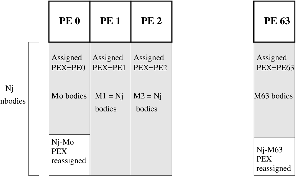
Figure 4: Dynamical Load Balance. PE executors assignment.

2.4.3 PEX reassignment.

During this phase each PE assigns a PEX to the $N_{\rm k}-M_{\rm k}$ remaining bodies (if any). Each PE follows this rule for the PEX assignment: for each of the remaining bodies all the processors (including the processing one) are put on a list, and the PEX is assigned to that PE having the smaller load.
In this way it turns out to be possible to minimize the $T_{\rm sol}$ in eq. 1 minimizing the $T_{\rm da}$ term. The use of this technique of Load Balancing results in a gain from 10% up to 25%.

2.5 Memory Requirements.

The memory requirements of the Tree N-body codes are generally large due to the presence of arrays containing the particles and the tree cells properties. In a Locally-Essential-Tree-based code, the larger part of the memory occupancy is due to the dimension of arrays containing the local particles’ and tree cells properties. Moreover a relevant part of memory occupancy must be used for the additional arrays containing particles and cells imported from other processors. This quantity increases with decreasing $\theta$ and is not a priori predictable, so that all the arrays must be dimensioned for the worst case.
In our work-memory/shared code the memory occupancy is lesser, because the absence of Locally Essential Trees reduces the replication of arrays. Let $N_{\rm bodies}$ be the number of particles. The memory occupancy of our code is given by:

$${\rm M}=\frac{40N_{\rm bodies}}{N_{\rm PE}}+5\frac{N_{\rm bodies}}{C}$$ (5)

words (1 word=8 bytes) for each PE. In the above equation $N_{\rm PE}$ is the number of PEs involved in the simulation and C a factor depending on the length of the interaction list formed by each particles during the tree traversal phase. An upper minimum value for this latter quantity is N/10. Using this value of C and for a total number of 256 PEs , it is possible to run a simulation with about $N_{\rm bodies}\approx 10^{6}$ on resources like those offered by the CINECA T3D (128 PEs, 2 Gbytes RAM). In the nearest future, using the T3E machine with 16 Mword for each node, more than 20 million particles simulation may be run. These figures may increase for $C>10$, and this fact opens the possibility of performimg simulations with 30-40 million particles even on MPP system having a moderate amount of mass memory e.g. of the order of a few distributed Gbytes.

3 Results

In order to compare the performance of our code in realistic situations we have run tests for both homogeneous and inhomogeneous initial conditions . At variance with the Molecular Dynamics case, the gravitational force induces an irreversible evolution towards highly clustered configurations. From the computational point of view this results into load imbalance, so a comparison of the two cases provides information on the efficiency of the Dynamical Load Balance procedure described before.
The central subroutine STEPSYS which advances the system’s positions and velocities of one time step can be schematically decomposed into three main phases: a) MAKETREE, where the oct-tree is builded; b) ACCGRAV, in which each particle inspects the tree, builds up an interaction list, and the acceleration on each particle is computed; c) STEPPOS and STEPVEL, where the system is advanced. This latter step is executed in parallel by each PE.
Following Warren and Salmon [13], we present our results plotting the quantity:

$$T_{\rm speed}=\frac{T_{\rm step}N_{\rm PE}}{N_{\rm bodies}}$$ (6)

where $T_{\rm step}$ is the normalized average execution time of STEPSYS over 10 time steps (measured w.r.t. the serial case). In an ideal case, one would expect that $T_{\rm step}\propto N_{\rm PE}^{-1}$. For the serial code one also expects: $T_{\rm step}\propto N_{bodies}logN_{bodies}$.

=#1 0.5#1

Figure 5: Scalability of the relative speedup for different partitions. $T_{step}$ is normalized to the value measured for 1 PE.

As one can see from Fig. 5, the code scales very efficiently for large number of particles: $T_{\rm speed}$ reaches an asymptotic regime already at $N_{\rm bodies}\approx 2\times 10^{5}$. It is interesting to observe that the asymptotic regime is reached also for high granularity cases, i.e. for $N_{\rm PE}=8,16$. The same trend concerning the scalability with $N_{\rm bodies}$ is observed for the scalability with $N_{\rm PE}$ (Figure 6). The anomalous behaviour of the run at 32k, visible also as a ‘shoulder’ at the corresponding point in Fig. 5, is due to spurious cache effects.

=#1 0.5#1

Figure 6: Scalability of the relative speedup for different sizes of the running code. $T_{step}$ is normalized as in Figure 5

In Figure 6 we plot the relative speedup $T_{\rm speed}$ as a function of $N_{\rm PE}$ for homogeneous inital conditions.
Note that $T_{\rm speed}$ provides a measure of the scalability of the code, not of its absolute speedup. This latter is plotted in Figure 7 for the subroutine ACCGRAV. Note that measuring ACCGRAV we are in fact measuring the performance of TREEWALK, the most time-consuming subroutine and the one which is fully parallelized. But the performance is also influenced by other factors, like those mentioned in section 2.1, which altogether act to reduce the absolute speedup. We believe however that it would be prove possible to increase futher the speedup with a dynamical tree allocation, and we are working along this direction. It is interesting to observe that our results for $T_{\rm speed}$ are comparable to those obtained by Warren and Salmon [13] (their Fig. 8). We cannot say very much about their absolute speedups, because they do not give any information about it.

=#1 0.5#1

Figure 7: Speedup for ACCGRAV.

As we mentioned at the beginning, Load Balancing is also necessary in order to avoid the performance degradation one meets when the system starts to cluster. In figure 8 we can appreciate how much this problem quantitatively affects . The quantity $T_{\rm step}$ almost doubles when one passes to clustered configurations, and also the steepness of the curves tends slightly to increase, although not dramatically. This means that the scaling properties of the codes keep almost unchanged with increasing clustering, and that even for highly inhomogeneous configurations there is not a significant increase of the communication overhead among the main sources of load unbalance.

4 Conclusions

The work- and memory-shared Tree N-body code we have described in this paper has some very interesting features. First, its memory occupancy is comparatively lesser than in a LET-based scheme, because in this latter some parts of the local trees have to be replicated on other PEs. This reduced memory occupancy results also in a reduced communication overhead, simply because the structures relevant for the force calculation are already shared and they have not to be exchanged as in the LET, message passing schemes. Being based on a different algorithm, the scalability of our code cannot be a priori assumed to be the same as for explicitly message-passing implementations as those developed by many authors [10, 2, 11, 13, 5].

=#1 0.5#1

Figure 8: Performance degradation with increasing clustering.

We observe however that as far as scalability (measured by $T_{\rm speed}$) is concerned, our code performs very well, in a way very similar to that observed in LET-based implementations. We think that a dynamical tree allocation, i.e. a scheme in which the block distribution of the tree changes with time, could increase the absolute speedup. The atomic, almost uniform distribution scheme we have adopted was motivated by the very good scalability, but in very inhomogeneous situations it could happen that a body residing in a given PE needs to access data from ‘deep’ cells lying on some far PE. Due to synchronization mechanisms this can occasionally result in a general slowing down of the code.
Our main purpose in this paper was to try to understand with specific tests these problems and how they affect the relative performance of different parts of the code. In a forthcoming paper [1] we will discuss a Load Balancing scheme based on a dynamic data sharing distribution scheme.

References

- [1] V. Antonuccio-Delogu, U. Becciani, G. Erbacci and A. Pagliaro, in preparation (1996)
- [2] Antonuccio-Delogu, V. and Becciani, U., ”A Parallel Tree N-Body Code for Heterogeneous Clusters”, in: J. Dongarra and J. Wasniewsky, eds.,Parallel Sciebtific Computing - PARA ’94 (Springer Verlag: 1994), 17
- [3] J. Barnes and P. Hut, Nature 324 (1986) 446
- [4] Cray Research Inc., ”Cray MPP Fortran Refeference Manual SR-2504 6.1 (1994)
- [5] J. Dubinski, ”A Parallel Tree Code”, submitted to New Astronomy (1996)
- [6] Gouhong Xu, ”A new parallel N-body gravity solver: TPM”, Astrophys. J. Supp. 97 (1995) 884
- [7] A. Geist, A. Beguelin, J. Dongarra, W. Jiang, R. Manchek and V. Sunderam, ”PVM 3 User’s Guide and Reference Manual”, ORNL/TM-12187, September 1994
- [8] V. Lamsani, L. Bhuyan and D. Scott Linthicum, Parallel Computing 21 (1995) 993
- [9] L. Hernquist, Astrophys. J. Suppl. 64 (1987) 715
- [10] J.K. Salmon, ”Parallel hierarchical N-body methods”, Ph. D.. Thesis, unpublished (California Institute of Technology: 1991)
- [11] J.K. Salmon and M.S. Warren, ”Skeletons from the Treecode closet”, J. Comp. Phys. 111 (1995) 136
- [12] L. Stiller, L.L. Daemene and J.E. Gubernatis, J. Comp. Phys. 115 (1994) 550
- [13] M.S. Warren and J.K. Salmon, ”A portable Parallel N-body code”, unpublished , (California Institute of Technology: 1995)
- [14] W.H. Zurek, P.J. Quinn, J.K. salmon and M.S. Warren, Astrophys. J 431 (1994) 559