ADP-AT-96-9 (Revised)
                                                                       J. Phys. G: Nucl. Part. Phys., submitted

Short Title: Cosmic-ray electrons and diffuse gamma-ray spectrum

PACS Numbers:

98.70.Sa Cosmic-rays (including sources, origin, acceleration, and interactions)

95.85.Pw Gamma-ray

98.70.Vc Background radiations

Abstract

The bulk of the diffuse galactic gamma-ray emission above a few tens of GeV has been conventionally ascribed to the decay of neutral pions produced in cosmic-ray interactions with interstellar matter. Cosmic-ray electrons may, however, make a significant contribution to the gamma-ray spectrum at high energies, and even dominate at TeV–PeV energies depending on their injection spectral index and acceleration cut-off energy. If the injection spectrum is flat, the highest energy electrons will also contribute a diffuse hard X-ray/soft gamma-ray flux via synchrotron emission, and this may offer an explanation for the OSSE observation of a steep spectrum below a few MeV from the inner Galaxy. We perform a propagation calculation for cosmic-ray electrons, and use the resulting interstellar electron spectrum to obtain the gamma-ray spectrum due to inverse Compton, synchrotron and bremsstrahlung interactions consistently from MeV to PeV energies. We compare our results with available observations from satellite-borne telescopes, optical $\check{\rm C}$erenkov telescopes and air shower arrays and place constraints on the injection spectrum of cosmic-ray electrons. With future observations at TeV–PeV energies it should be possible to determine the average interstellar spectrum of cosmic-ray electrons, and hence estimate their spectrum on acceleration.

1 Introduction

Cosmic-rays with energies up to $\sim 100$ TeV are thought to be accelerated by the 1st order Fermi mechanism at supernova shocks (see Jones and Ellison [1] for a recent review), and recently the EGRET instrument on the Compton Gamma-Ray Observatory has detected gamma-ray signals above 100 MeV from at least two supernova remnants (SNR) $-$ IC 443 and $\gamma$ Cygni [2]. Further evidence for particle acceleration comes from recent ASCA observations of non-thermal X-ray emission from SN 1006 [3], and correlation of ASCA and ROSAT observations of non-thermal X-ray emission from IC 443 [4]. Reynolds [5] and Mastichiadis [6] interpret the former as synchrotron emission by electrons accelerated in the remnant up to energies as high as 100 TeV, while Keohane et al [4] argue that the latter is due to synchrotron emission by electrons accelerated to $\sim 10$ TeV. Recently Pohl [7] has suggested electron acceleration up to 100 TeV energies may not be unique to SN 1006, and that other acceleration sites of high energy electrons probably exist in the Galaxy.

Electrons accelerated to 100 TeV energies would eventually escape their acceleration sites and diffuse in the Galaxy, cooling through synchrotron radiation and inverse Compton (IC) scattering on the galactic magnetic and radiation fields respectively. For synchrotron cooling, electrons of these energies in a magnetic field strength $\sim 6$ $\mu$G would give a diffuse flux of radiation in the X-ray regime, while IC scattering of 100 TeV energy electrons on the cosmic microwave background radiation (CMBR) would give a diffuse flux of gamma-rays at TeV energies. The spectrum of radiation produced by these processes is dependent on the high energy interstellar electron spectrum, which in turn is dependent on the initial source spectrum, distribution of sources and propagation. If this radiation is detectable it would provide a means of estimating the average interstellar electron spectrum, and hence the spectrum of electrons at acceleration.

Protheroe and Wolfendale [8], in an approximate calculation, have considered the dual role of ultrarelativistic electrons in producing the diffuse galactic radiation from hard X-rays to TeV energies and above, and an analysis of Uhuru data by Protheroe et al [9] has indicated a considerable contribution by synchrotron emission in the soft X-ray band. However, more recent calculations of the diffuse gamma-ray spectrum [10, 11, 12, 13, 14] have generally neglected synchrotron emission as a significant production process. Inverse Compton scattering on the ambient galactic photon fields, on the other hand, is recognised as a important contributor to the diffuse gamma-ray spectrum at MeV to GeV energies. In particular, detailed predictions of IC gamma-rays above $70-100$ MeV have been made by Bloemen [15] and Chi et al [16], with estimates of the contribution by this component being up to $\sim 50\%$ of the diffuse intensity at medium galactic latitudes ($|b|=10^{\circ}$ to $20^{\circ}$). An analysis of EGRET data by Giller et al [17] has suggested a contribution by IC of $\sim 30\%$ for medium latitudes, and up to $\sim 45\%$ toward the galactic pole, in the energy range $30-4000$ MeV. Strong et al [12] have shown that an IC component is required to provide a good fit to the gamma-ray data from 1 MeV to 1 GeV; see also Bertsch et al [10] and Hunter et al [14].

In this paper we consider possible injection spectra of primary cosmic-ray electrons, and the resulting diffuse gamma-ray spectrum of the Galaxy. Starting with a power-law spectrum of electrons at acceleration, we propagate electrons in the Galaxy using a diffusion model which is consistent with the observed cosmic-ray secondary to primary data and ¹⁰Be abundance to obtain the interstellar electron spectrum. Realistic models of the galactic matter distribution, magnetic field and interstellar radiation field (ISRF) are used in the propagation calculation. Inverse Compton, bremsstrahlung and synchrotron production spectra are calculated using the electron spectra resulting from the propagation calculation, and we give a consistent treatment of high energy photon production by these processes from keV to PeV energies. Our predictions are then compared with satellite observations at keV to GeV energies [12, 18, 19, 20, 21, 22], optical $\check{\rm C}$erenkov telescope observations at TeV energies [23] and air shower observations [24, 25, 26] at $50-1000$ TeV energies.

In Section 2 we describe an efficient Monte Carlo method that allows us to vary source distributions, or injection spectra, without having to repeat the propagation calculation for each different case. We then use the method to obtain the interstellar electron spectrum for representative regions of the Galaxy. We consider various injection spectral indices, and constrain the model spectra using direct measurements of the local electron spectrum and the galactic non-thermal radio emission. Electron spectra that satisfy the constraints are then used in Section 3 to calculate production spectra for IC, bremsstrahlung and synchrotron emission processes, and to obtain the expected gamma-ray intensity. In Section 4 we discuss the limitations of our model, and the implications of our predictions.

2 The Electron Propagation Calculation

2.1 Numerical Method

The standard transport equation for cosmic-ray electrons undergoing continuous energy losses is [27]

$$\frac{\partial n\left(E,\vec{r},t\right)}{\partial t}=q\left(E,\vec{r}\right)+K(E)\nabla^{2}n\left(E,\vec{r},t\right)+\frac{\partial}{\partial E}\left[n\left(E,\vec{r},t\right)\frac{dE}{dt}\right]$$ (1)

where $n\left(E,\vec{r},t\right)$ is the number density of electrons, $q\left(E,\vec{r}\right)$ is the source function of cosmic-ray electrons assuming a constant injection rate, the second term on the right represents energy dependent spatial diffusion of the electrons with scalar diffusion coefficient $K(E)$ and the third term represents the continuous energy losses of the electrons. We seek steady state solutions $n\left(E,\vec{r}\right)$ and solve Equation 1 by Monte Carlo methods which we describe below.

Consider electrons of energy $E^{\prime}$ released at $\vec{r}\,^{\prime}$ to diffuse through the Galaxy and continuously lose energy by interacting with the background radiation, magnetic field and matter. We define $p(E,\vec{r};E^{\prime},\vec{r}\,^{\prime})$ to be the probability density (cm^-3) at $\vec{r}$ of points in space at which the energy of the electrons was precisely $E$. Given the energy-loss rate

$${dE\over dt}=-b(E,\vec{r})\hskip 14.22636pt{\rm(GeV\;s^{-1})},$$ (2)

the average time spent with energy between $E$ and $(E+dE)$ is $dE/b(E,\vec{r})$ if the electron is located at or close to $\vec{r}$. Hence, the average time spent by an electron with energies between $E$ and $(E+dE)$ per unit volume at $\vec{r}$ is $p(E,\vec{r};E^{\prime},\vec{r}\,^{\prime})dE/b(E,\vec{r})$. Thus, for some source distribution $q(E,\vec{r})$ (GeV^-1 cm^-3 s^-1) we obtain the number density of electrons $n(E,\vec{r})$ (GeV^-1 cm^-3) at $\vec{r}$

$$n(E,\vec{r})=b(E,\vec{r})^{-1}\int dV^{\prime}\int_{E}^{\infty}dE^{\prime}q(E^{\prime},\vec{r}\,^{\prime})p(E,\vec{r};E^{\prime},\vec{r}\,^{\prime}).$$ (3)

The most time-consuming part of the calculation is working out $p(E,\vec{r};E^{\prime},\vec{r}\,^{\prime})$ because this contains all the information about propagation, energy losses and interactions during propagation.

We make the approximation that propagation takes place only in the $z$ direction (perpendicular to the galactic plane), and use a two-dimensional model of the radiation field, magnetic field, and matter density, in which these quantities depend on galactocentric radius, $R$, and height above the plane, $z$. For this case

$$n(E,R,z)\approx b(E,R,z)^{-1}\int dz^{\prime}\int_{E}^{\infty}dE^{\prime}q(E,R,z^{\prime})p(E,R,z;E^{\prime},R,z^{\prime})$$ (4)

where the $R$ dependence has been retained due to the two-dimensional dependence of the matter distribution, radiation and magnetic fields. The probability density $p(E,R,z;E^{\prime},R,z^{\prime})$, which we shall refer to as the “probability matrix”, is essentially the Green’s function for Equation 1 and is calculated by the Monte Carlo method as described later. We can re-use $p(E,R,z;E^{\prime},R,z^{\prime})$ to obtain $n(E,R,z)$ for different source spectra or distributions $q(E,R,z)$ simply by performing the integrals over energy and volume given above. This is particularly useful if we wish to consider different cosmic-ray electron source spectra.

To demonstrate the reliability of our method we calculate $n(E,R,z)$ for two simple cases, and compare with the analytical solutions. We consider: (i) the solution of Equation 1 with energy independent diffusion coefficient $K$ and constant energy loss rate $b(E,R,z)=\alpha$, and (ii) the solution of Equation 1 with energy dependent diffusion coefficient $K(E)=K(E/E_{0})^{\delta}$ and energy loss rate $b(E,R,z)=BE^{2}$. The motivation for this is that cases (i) and (ii) approximate the diffusion and energy loss mechanisms of cosmic-ray electrons at low and high energies respectively. For simplicity we obtain the solution $n(E,R,z)$ for both cases without boundaries.

The Green’s function for case (i) is [28]

$$G_{(i)}(E,R,z;E^{\prime},R,z^{\prime})=\frac{q_{0}}{\sqrt{4\pi K\alpha\left|E-E^{\prime}\right|}}\exp\left(-\frac{\alpha\left(z-z^{\prime}\right)^{2}}{4K\left|E-E^{\prime}\right|}\right)$$ (5)

and for case (ii)

$$G_{(ii)}(E,R,z;E^{\prime},R,z^{\prime})=\frac{q_{0}}{\sqrt{4\pi B^{2}E^{4}(\lambda(E)-\lambda(E^{\prime}))}}\exp\left(-\frac{(z-z^{\prime})^{2}}{4(\lambda(E)-\lambda(E^{\prime}))}\right)$$ (6)

where $\lambda(E)=-\int_{E}^{\infty}K(X)/b(X,R,z)dX$. By definition, the Green’s functions are solutions of Equation 1 for a source function $q(E,z)=q_{0}\delta(E-E^{\prime})\delta(z-z^{\prime})$ (GeV^-1 cm^-3 s^-1).

In the Monte Carlo method, for each case we obtain $p(E,R,z;E^{\prime},R,z^{\prime})$ with the same source function. For case (i) we take 41 energy bins at intervals of $\Delta\log E=0.1$ with mid-bin energy starting at $10^{-3}$ GeV. The Monte Carlo procedure is as follows. A particle is injected at $z=0$ with initial energy $E_{j}$. Based on random walk theory and its relation to diffusion [29], the diffusion in $z$ is simulated by multiplying a randomly sampled normal deviate, $\zeta$, by the standard deviation

$$\sigma_{z}={\rm min}\left(\sqrt{2K\Delta t},\sigma_{z_{max}}\right)$$ (7)

where $\Delta t=\Delta E/b(\sqrt{E_{j}E_{j-1}},R,z)$ with $\Delta E=(E_{j}-E_{j-1})$ being the difference between the current mid-bin energy and the next lowest mid-bin energy, and $\sigma_{z_{max}}$ is the maximum standard deviation and is chosen to minimise computing time while ensuring the Monte Carlo and analytical results agree; $\sigma_{z_{max}}$ is chosen to be small compared to the distance over which physical parameters of the model change significantly. The new position is obtained by adding $\Delta z=\zeta\sigma_{z}$ to the current position. If $\sigma_{z}<\sigma_{z_{max}}$ the particle’s energy is set to $E_{j-1}$ and, if the new position is in the “observing region” i.e. the region for which we wish to obtain $n(E,R,z)$, the particle is recorded as having been observed with energy $E_{j-1}$. Otherwise, if $\sigma_{z}=\sigma_{z_{max}}$, the energy lost by the particle while diffusing is calculated and subtracted from its current energy. If the particle’s energy falls below $E_{j-1}$, the approximate position where its energy became lower than $E_{j-1}$ is determined and, if this position is within the observing region, the particle is recorded as having been observed with energy $E_{j-1}$. The energy bin counter $j-1$ is then decremented by 1, and the above procedure is repeated until the particle reaches some large distance away from the galactic plane, taken to be 20 kpc in this instance; particles diffusing out to this distance would have lost an amount of energy large enough to place them below the lowest particle energy in the simulation, hence they are no longer of interest. The probability matrix is computed by injecting $N$ particles in each of the source energy bins and following the Monte Carlo procedure outlined above, the final result being divided by $N$ and the volume of the observing region. Figure 1a compares the distribution of particles in $E$ and $z$ for source energies $E^{\prime}=10^{-0.4}$ GeV calculated using the above method for $N=10^{5}$ particles and $\sigma_{z_{max}}=50$ pc, and with Equation 5 for $q_{0}=1$ cm^-2 s^-1, $K=2.5\times 10^{28}$ cm² s^-1 and $\alpha=5\times 10^{-16}$ GeV s^-1.

For case (ii) we take 61 energy bins at intervals of $\Delta\log E=0.1$ with mid-bin energy starting at $10^{0}$ GeV, and follow the Monte Carlo procedure outlined above. Figure 1b compares the distribution of particles in $E$ and $z$ for source energies $E^{\prime}=10^{6}$ GeV obtained from the probability matrix calculated using the Monte Carlo method with the analytical result (Equation 6) for $N=10^{5}$ particles, $\sigma_{z_{max}}=50$ pc, $q_{0}=1$ cm^-2 s^-1, $K=2.5\times 10^{28}$ cm² s^-1, $E_{0}=3$ GeV, $\delta=0.6$ and $B=9.12\times 10^{-17}$ GeV^-1 s^-1.

In both cases the agreement between the Monte Carlo and analytical results is excellent. The particular choice of $\sigma_{z_{max}}$ used above was found to give the best compromise, minimising computing time while maintaining good agreement with the analytical results. Making $\sigma_{z_{max}}$ much larger resulted in the particle distribution at low observing energies falling below the analytical results, while making it smaller ensured accuracy but produced unacceptably long run-times for the number of particles chosen. Similarly simulations were performed for varying $N$ and, in conjunction with our choice of $\sigma_{z_{max}}$, it was found $N=10^{5}$ particles yielded the best compromise for computing time versus statistical accuracy.

2.2 Calculated Electron Spectra

For the propagation calculation we adopt a halo half-height of 3 kpc [30], and use a diffusion coefficient which is constant at $2.5\times 10^{28}$ cm² s^-1 below a magnetic rigidity of $\rho=3$ GV and increases as $(\rho/3{\rm\;GV})^{0.6}$ above 3 GV [31]. The modified source distribution of Webber et al [32] is used for the radial distribution of primary cosmic-ray electron sources. The sources are assumed to be uniformly distributed in $z$ with a half-height of 0.15 kpc comparable to the scale height of SNR [33].

Theories of cosmic-ray acceleration predict a power-law dependence for the injection spectrum of particles $q(E)\propto E^{-\gamma}$ [1]. Studies of the non-thermal radio emission of the Galaxy give the following values for the power-law spectral index ($I_{\nu}\propto\nu^{-\alpha}$): $\alpha=0.55-0.6$ at 5 to 80 MHz in the direction of the galactic pole [34]; $\alpha=0.5-0.6$ at 38 to 408 MHz over the northern galactic hemisphere [35]; $\alpha=0.7$ for 408 to 5000 MHz for low latitudes toward the inner Galaxy [36]; and $\alpha=0.85$ in the plane, increasing to $\alpha=1.0$ at higher latitudes for 408 to 1020 MHz [37]. Given the relationship $\alpha=(\gamma-1)/2$ we see $\gamma=2-3$ using the published ranges. Due to the continuous energy losses suffered by electrons the source spectrum is not uniquely determined from the radio emission. We therefore consider values of $\gamma$ at injection in the range 2 to 2.4.

Throughout this paper, we take the galactocentric radius of the Sun to be $R_{S}=8.5$ kpc. Where the empirical models we use in our calculations use a different $R_{S}$ we scale them appropriately to our adopted value. The maximum extent of the Galaxy in $R$ is taken to be 16 kpc.

For the ambient radiation fields of the Galaxy we use the model of Chi and Wolfendale [38] for the ultraviolet to near infra-red (‘optical’), the cold dust emission curve of Cox et al [39] for the far infra-red, and we take the temperature of the CMBR as 2.735 K. For electron interactions with matter we model three components of the interstellar medium: the distribution of HI as given by Dickey and Lockman [40] with column density $\int n_{\rm HI}dz$ = $6.2\times 10^{20}$ cm^-2 and a FWHM of 0.23 kpc at $R_{S}$; the H₂ distribution of Bronfman et al with column density $\int n_{\rm H_{2}}dz$ = $3.8\times 10^{20}$ cm^-2 and a FWHM of 0.14 kpc at $R_{S}$; and the HII distribution of Reynolds [42, 43, 44] with column density $\int n_{\rm HII}dz$ = $2\times 10^{20}$ cm^-2 and a FWHM of 3 kpc at $R_{S}$. A contribution by helium consistent with the observed abundance is also included. The concentric ring model of Rand and Kulkarni [45] is used for the regular component of the galactic magnetic field and we adopt the value of 5 $\mu$G derived by these authors for the magnitude of the random component. Energy loss formulae in both the non-relativistic and relativistic case for the various interactions electrons can undergo with the interstellar medium, radiation and magnetic fields are taken from Ginzburg and Syrovatskii [27]; we consider ionisation loss and bremsstrahlung on both the neutral and ionised medium, and synchrotron and IC losses. For high energies the IC energy losses on the ISRF are in the Klein-Nishina regime and we calculate the energy loss rate using Monte Carlo methods as described by Protheroe [46].

We divide the Galaxy up into radial bins of half-width 1 kpc centred on $R$ = 1, 3, 5, 7, 9, 11, 13 and 15 kpc. The propagation parameters for each radial bin are then computed by averaging the models of the matter distribution, radiation and magnetic fields over the inner radius to the outer radius of each bin. The electron spectra calculated for each bin are then taken to be representative of that region of the Galaxy.

To obtain the probability matrix for the $i$-th radial bin, we take 111 energy bins at intervals of $\Delta\log E=0.1$ with mid-bin energy starting at $10^{-3}$ GeV. We inject particles uniformly within the source region and follow the Monte Carlo procedure outlined in the previous section. A value of $\sigma_{z_{max}}$ of 50 pc is used, and $N=10^{5}$ particles are injected at each of the source energy bins.

The interstellar electron spectrum is obtained from the probability matrix and the source spectrum using Equation 4. In Figure 2 we show a comparison of direct measurements of the electron intensity spectrum in the solar vicinity, spectra derived from non-thermal radio measurements and our predicted interstellar electron spectra with injection spectral indices $\gamma=2$, 2.2 and 2.4 normalised to the observed spectrum at 10 GeV [47, 48, 49] because for energies $\sim 10$ GeV and above solar modulation effects are believed to give only minor deviations from the interstellar spectrum, and the error bars on the measurements around 10 GeV are relatively small when compared with data at higher energies. We can see that a flat injection index such as $\gamma=2$ produces a local electron spectrum that neither agrees with the low energy spectrum derived from non-thermal radio measurements, nor with the high energy data above 20 GeV. A flat injection spectrum such as $\gamma=2$ is therefore, at least for the local region, ruled out, and we do not consider $\gamma=2$ any further except for a special case which is discussed in Section 3.3. Our predictions for $\gamma=2.2$ and 2.4 are reasonably consistent with the data from 100 MeV up to roughly 50-60 GeV, with $\gamma=2.2$ being slightly preferred by the spectrum derived from non-thermal radio observations. At higher energies both spectra gradually over-predict the data such that at 2 TeV a $\gamma=2.2$ spectrum is a factor of 3 higher and a $\gamma=2.4$ spectrum is a factor $\sim 1.5$ higher. However we have assumed a continuous source distribution at all energies, and this is unlikely to be valid locally as discussed below.

Electrons are assumed to be accelerated at strong supernova shocks, and the nearest source region may be $\sim 100$ pc or more away. At energies where the energy-loss time scale is less than or comparable to the diffusion time to the nearest source high energy electrons will lose most of their energy before reaching the observer. The local spectrum will then be significantly steeper than the average interstellar spectrum [8]. Detailed calculations by Aharonian et al [50] and Atoyan et al [51] have shown that such a steepening occurs when the inhomogeneity of the source distribution is taken into account. However for X-rays and gamma-rays produced by electrons interacting with the galactic matter distribution, radiation and magnetic fields, the spectrum of radiation observable at Earth depends on many contributions by the various X-ray and gamma-ray production processes along the line-of-sight. This samples the spectrum of X-rays and gamma-rays, and hence the spectrum of electrons producing them, over large scales, and effectively smooths out local inhomogeneities in the electron spectrum that could arise due to an uneven source distribution. Therefore, at least in a first analysis, a continuous distribution of sources is reasonable when discussing gamma-ray observations.

As a consistency check on our electron spectra, we calculate the non-thermal emission in the direction of the galactic pole. We compare our predictions with the results of Broadbent et al [54], who derive a galactic pole brightness temperature of 12.3 K from modeling the 408 MHz sky maps of Haslam et al [55], and with the results of Lawson et al [35] at 38 MHz and Reich and Reich [37] at 1420 MHz. We show our predicted non-thermal spectrum at the pole in Figure 3 together with the experimental results. Our results are within a factor of 1.5 of the data, indicating our electron spectra and magnetic field distribution are not unreasonable. We use our calculated electron spectra in the next Section to obtain X-ray and gamma-ray emissivities for synchrotron, bremsstrahlung and IC radiation, and use these to compute diffuse galactic radiation spectra and compare with experimental results.

3 Diffuse Galactic Gamma-Ray Spectra

3.1 Diffuse Gamma-Ray Emissivities

Our first step is to calculate the emissivity spectra of gamma radiation due to electron interactions with the interstellar medium, radiation and magnetic field. We calculate the IC, bremsstrahlung and synchrotron contributions to the diffuse gamma radiation from low to very high energies. Emissivity spectra for the three processes are calculated using

$$q_{{}_{\rm Brem,IC,Sync}}\left(E_{\gamma},\vec{r}\right)=\frac{4\pi}{c}\int^{E_{\rm max}}_{E_{\rm min}}J\left(E,\vec{r}\right)\frac{dN_{\rm Brem,IC,Sync}}{dtdE_{\gamma}}dE\hskip 14.22636pt({\rm GeV^{-1}\;cm^{-3}\;s^{-1}})$$ (8)

where $J(E,\vec{r})$ (GeV^-1 cm^-2 s^-1 sr^-1) is the interstellar electron spectrum, and $dN/dtdE_{\gamma}$ is the production spectrum for the appropriate process. We calculate $dN/dtdE_{\gamma}$ for bremsstrahlung produced by electrons interacting with neutral and ionised hydrogen, and neutral helium. For IC gamma-rays $dN/dtdE_{\gamma}$ is evaluated using the Klein-Nishina cross-section. Formulae for calculating $dN/dtdE_{\gamma}$ and the appropriate integration limits are given by Blumenthal and Gould [56] for bremsstrahlung and IC radiation, and by Pacholczyk [57] for synchrotron radiation.

Figure 4 shows the local emissivity per interstellar H atom due to interactions with matter. The dotted curves show our results for bremsstrahlung for the two injection spectra, and the chain curve shows the expected contribution from $\pi^{0}$-decay according to Stecker [58] as parameterised by Bertsch et al [10]. We also show the local emissivity per interstellar H atom estimated from EGRET data (Strong and Mattox [22]), COMPTEL data (Strong et al [12, 19]) and COS-B data (Strong et al [18]). A reasonable fit to the low energy data is obtained for an injection index $\gamma=2.4$, with the gamma-ray emissivities for $\gamma=2.2$ being a factor of $\sim 2$ too low when compared with the data. There is, however, some uncertainty in the COMPTEL spectrum amounting to a possible factor of two over-estimation [59]. With this taken into account a $\gamma=2.2$ spectrum is allowed by the data. As noted in several other papers [12, 14, 22], above 500 MeV up to 10 GeV, the predicted emissivity due mainly to $\pi^{0}$-decay (not calculated in this paper), while consistent with the COS-B data, is significantly below the EGRET data.

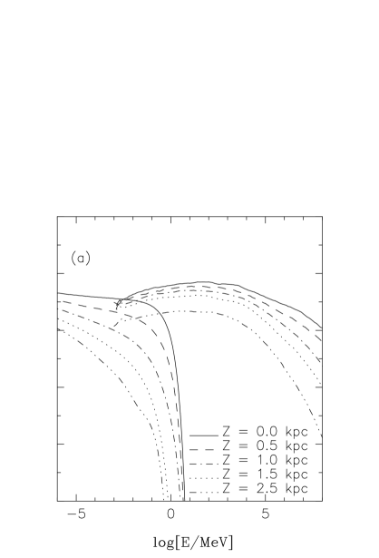
Figure 5: Variation of the synchrotron and IC emissivity with height above the Galactic plane for the radial bin centred on $R=9$ kpc and an injection spectrum of (a) $E^{-2.4}$ and (b) $E^{-2.2}$. Emission spectra have been calculated using injection spectra with a maximum injection energy cut-off at 1 PeV.

Figure 5 shows the variation with height above the galactic plane of the IC and synchrotron emissivities for the local region calculated for a high energy cut-off in the injection spectrum at 1 PeV; a cut-off in the injection spectrum of electrons at 100 TeV to 1 PeV would be expected if electrons are accelerated by SNR [60, 61, 62]. Self-consistency for both the IC and synchrotron contributions is ensured by using the same galactic radiation field and magnetic field models for the emissivity calculation as used in the electron propagation. As can be seen in the Figure, synchrotron radiation can contribute significantly to the emission in hard X-rays, being at least comparable to the IC emission for energies $<100$ keV in the galactic plane; at greater heights above the galactic plane the synchrotron spectrum decreases more rapidly than the IC spectrum because the distribution of very high energy electrons producing the synchrotron emission is significantly diminished away from the plane, whereas the distribution of relatively low energy electrons producing the IC spectrum extends to a considerable height above the plane. Variation of the injection spectrum index from $\gamma=2.4$ to 2.2 increases the synchrotron emission, and additionally tends to flatten the IC spectrum at high energies. Furthermore, the cut-off in the synchrotron spectrum is directly linked to the cut-off in the injection spectrum of electrons: a lower cut-off in the electron injection spectrum gives a correspondingly lower cut-off in the synchrotron spectrum. This raises the interesting possibility of detecting signatures of maximum acceleration energies of electrons using the galactic diffuse hard X-ray background.

3.2 Diffuse Gamma-Ray Intensities

We use the emissivities calculated in the previous section to predict the intensity spectra for various gamma-ray production mechanisms, and compare with observation. We calculate the average spectrum for the inner Galaxy, and show this in Figure 6 for the two injection spectra. Also shown are data from COS-B [18], COMPTEL [12], EGRET [22] and OSSE [12, 20]. For the bremsstrahlung and $\pi^{0}$-decay spectra we have used the HI and CO gas survey data from [18] to obtain the average intensity. For the synchrotron intensities we have used electron spectra with cut-offs of the maximum injection energy at 100 TeV and 1 PeV respectively. The EGRET excess above 500 MeV apparent in the emissivity spectrum is also present in the intensity spectrum, and our calculations indicate no simple modification in the electron spectrum can account for this feature. Also it should be borne in mind that the uncertainty in the COMPTEL emissivity spectrum mentioned in the previous section applies also to the COMPTEL intensity spectrum, i.e. it may be a factor $\sim 2$ too high [59]. It can be seen that a $\gamma=2.4$ electron spectrum produces an intensity spectrum which is largely consistent with the satellite data above 1 MeV, however it is unable to provide an explanation for the much softer gamma-ray spectrum observed by OSSE.

The fit to the data above 1 MeV for $\gamma=2.2$ is acceptable when the COMPTEL uncertainty is taken into account. In the hard X-ray range a flatter spectrum appears for a $\gamma=2.2$ spectrum due to the synchrotron emission by very high energy electrons in the galactic magnetic field, and is dependent on the cut-off in the primary injection spectrum of electrons, as noted in the previous section. For neither injection spectrum is the OSSE data well fitted, and it has been suggested that a new population of low energy electrons emitting bremsstrahlung radiation is required to provide the observed turn-up in the hard X-ray spectrum [13, 21, 63]. However, it was noted in Section 3.1 that flattening the electron injection index gave an enhanced synchrotron emission. If, for example, the injection spectrum in the inner Galaxy was flatter than that locally, a flatter interstellar electron spectrum would result, and this in turn would give an enhanced synchrotron emission. We return to this point in Section 3.3 when contrasting the hard X-ray and IC predictions.

At higher energies a dominant contribution by the IC component is of interest because the IC spectrum is directly related to the interstellar electron spectrum, which is itself directly related to the electron injection spectrum. At sufficiently high energies where the IC spectrum could be unambiguously detected, information about the electron injection spectrum can be obtained. The Figure indicates the IC emission in the inner Galaxy is dominant above 30 GeV for $\gamma=2.2$ and above 100 GeV for $\gamma=2.4$.

We have computed the spectrum in the direction $l=0^{\circ}$, $b=0^{\circ}$, and compared our predictions with recent calculations of the spectrum due to $\pi^{0}$-decay in the same direction [64, 65]. We show the comparison in Figure 7 where we have calculated IC spectra for $\gamma=2.4$ and $2.2$, and for high energy cut-offs of the injection spectrum at 100 TeV and 1 PeV, and with no cut-off. At energies above $\sim 100$ TeV the path-length of gamma-rays against photon-photon pair production on the CMBR is of the order size of the Galaxy. We therefore include attenuation on the CMBR when calculating our spectra; the difference between the attenuated and unattenuated spectra is shown in the top two branches of the $\gamma=2.2$ curve in the Figure. For energies in the range 1 MeV to 1 TeV the contribution by the IC process is predominantly due to scattering of optical and far infra-red photons. The optical component of the ISRF is the most uncertain due to the approximations used in the absorption calculation, and with estimates of the total luminosity varying by a factor of two [38, 66]. Furthermore, we do not attempt a detailed modelling of the ISRF in the wavelength range 8 $\mu$m to 50 $\mu$m, however this region of the ISRF is not as intense as the spectrum at shorter and longer wavelengths, and therefore contributes a comparatively small amount to the total energy density of the ISRF. Given the uncertainties in the optical component, and our approximation of the middle infra-red spectrum, our predictions for the 1 MeV to 1 TeV energy range will be accurate only within a factor of two. For higher energies, IC scattering of optical and far infra-red photons is in the Klein-Nishina regime, and so scattering of CMBR photons contributes to the bulk of the spectrum. Thus the uncertainty in our predictions due to uncertainties in the radiation field model diminishes at high energies. In the Figure we see that a $\gamma=2.4$ spectrum is at least comparable to the lowest of the $\pi^{0}$-decay predictions at 1 TeV (note the differences between the two $\pi^{0}$-decay predictions are due, in part, to the differences in the cosmic-ray spectrum and the pion multiplicities used), and that a $\gamma=2.2$ spectrum is about a factor of 3 higher than the $\gamma=2.4$ prediction at 1 TeV, increasing slowly with increasing energy. At the highest particle energies in our calculations the IC spectrum is at least of a similar magnitude to the largest $\pi^{0}$-decay predictions. Hence the gamma-ray intensity above 1 TeV can have a significant contribution due to IC scattering.

We calculate a longitude profile for the integral gamma-ray spectrum above 1 TeV and show this in Figure 8 together with the expected profile of $\pi^{0}$-decay gamma-rays as predicted by Berezinsky et al [64]. It can be seen the TeV gamma-ray intensity is sensitive to the electron injection spectrum. Additionally, introducing a high energy cut-off in the injection spectrum results in a well defined high energy cut-off in the IC spectrum as in Figure 7. Hence measurements of the diffuse gamma-ray spectrum beyond TeV energies may provide a direct means of estimating the electron source spectrum.

Upper limits on the diffuse gamma-ray spectrum for energies $\sim 50-500$ TeV have only been published for experiments located in the Northern Hemisphere. Observations of the galactic centre region are precluded by the location on Earth of these experiments. At $\sim 400$ GeV energies the Whipple group [23] have obtained upper limits on the ratio of the diffuse gamma-ray spectrum to the all particle cosmic-ray spectrum. At $\sim 50-500$ TeV energies the Utah-Michigan array [24] and CASA-MIA [26] have searched for diffuse emission in the region of the sky corresponding to the galactic coordinates $50^{\circ}<l<200^{\circ}$ and $|b|<10^{\circ}$, and have obtained upper limits on the ratio of diffuse gamma-rays to total cosmic-ray intensity. Published data for the HEGRA array [25] covers a region of sky that includes portions of the galactic plane as well as high galactic latitudes.

To make a proper comparison with the observational data, we have calculated the expected spectrum of diffuse IC radiation averaged over the region of the sky covered by the Utah-Michigan array and CASA-MIA, and the region of sky covered by the HEGRA array (being at a similar latitude, the Whipple Observatory covers a region of sky similar to that of the HEGRA array). We show our predictions in Figure 9 for the the two injection indices, together with cut-offs in the injection spectrum at 100 TeV and 1 PeV respectively, along with the upper limits for the diffuse gamma-ray spectrum obtained by converting the ratios $I_{\gamma}/I_{CR}$ from the above experiments to gamma-ray intensity upper limits using the all particle cosmic-ray spectrum [67]. The Whipple and HEGRA upper limits do not constrain either the injection index, or the cut-off in the injection spectrum. The CASA-MIA and Utah-Michigan upper limits, however, do at least allow us to rule out several of the cases considered. For example, injection energies beyond $\sim 500-700$ TeV are ruled out for a $\gamma=2.2$ injection spectrum. For a $\gamma=2.4$ spectrum no constraints are placed by the experimental results.

3.3 Possible explanation for the steep hard X-ray spectrum

We now contrast the very high energy IC predictions and the hard X-ray synchrotron results, and suggest a possible explanation for the steep hard X-ray spectrum. For an $E^{-2.4}$ injection spectrum, no constraints are placed by either the hard X-ray nor the IC predictions, and below 1 MeV the spectrum is not of the required shape and gives a poor fit to the data (see Figure 6). For this case, a new component of the galactic background radiation is needed at low energies to explain the turn up in the OSSE spectrum, and Skibo et al [13] have argued that a new population of non-thermal bremsstrahlung producing electrons with steep spectra ($\propto E^{-2.5}$) are required to explain the observed spectrum. Assuming the observed X-ray spectrum is truly diffuse, their approach suggests a power required to maintain the electrons against energy losses in the interstellar medium about an order of magnitude larger than that supplied by galactic supernovae [13, 63]. On the other hand the hard X-ray spectrum may be due to the sum of a large number of steep power-law unresolved point sources in which case the problems with the energetics in the Skibo et al model are circumvented. In any case an $E^{-2.4}$ spectrum is realistically only able to provide a good fit to the data between 1 MeV and $\sim 500$ MeV, with no constraints provided by the high energy IC spectrum.

For an $E^{-2.2}$ spectrum, the high energy spectrum is constrained by the CASA-MIA data: no electrons with energies greater than $500-700$ TeV can be accelerated. The hard X-ray predictions give no indication of a maximum injection energy cut-off, and at first glance the fit to the OSSE data seems not good enough to suggest a synchrotron origin for the hard X-ray spectrum. However in Section 3.1 we noted that as the injection spectrum flattened from $\gamma=2.4$ to 2.2 the magnitude of the synchrotron emission became correspondingly greater. If the injection spectrum was flattened further to, for example, $\gamma=2$ then the OSSE data may be able to be fitted. As our calculations in Section 2.2 indicated, such an injection spectrum gives an interstellar electron spectrum inconsistent with the local one, and this would seem to be not allowed. This assumes a single injection index adequately describes electron acceleration over the entire Galaxy. However, toward the inner Galaxy, in regions of greater star formation, there could be a large population of unresolved young SNR with relatively flat injection spectra, and these could give the required spectrum toward the inner Galaxy; it must be borne in mind that the CASA-MIA results are for the galactic disk $50^{\circ}<l<200^{\circ}$ which excludes most of the inner region of the Galaxy. Towards the outer Galaxy the star formation rate is not as great, and the SNR located in this region are sparser and there are probably fewer in the early stages off their evolution, and hence most are less efficient accelerators of electrons [68]. This could give a steeper injection spectrum towards the outer Galaxy than the inner Galaxy.

We have computed average gamma-ray spectra for both the inner Galaxy and the region of sky covered by CASA-MIA using a ‘modified’ source model comprising of an $E^{-2}$ injection spectrum for $R<6$ kpc, and an $E^{-2.2}$ injection spectrum for $R>6$ kpc; we re-use the probability matrix for the appropriate radial bin together with the modified source model to obtain electron spectra for the Galaxy, as described in Section 2.2. In the absence of truly three-dimensional diffusion in our calculations we obtain the normalisation for the electron spectra in the inner Galaxy by normalising to the local data around 10 GeV, and then scaling according to the distribution of SNR from Section 2.2 ; this, at best, approximate method at least allows us to demonstrate how a fit to the gamma-ray spectra might be obtained. We show our prediction for the inner region of the Galaxy using this combination of injection spectra in Figure 10. The fit to the diffuse hard X-ray to gamma-ray spectrum is greatly improved (bearing in mind the possible COMPTEL uncertainty) and could be made to give an even better fit with minor changes to the model input. For the outer region of the Galaxy (not plotted) we obtain a high energy spectrum which is almost identical to the $\gamma=2.2$ spectrum in Figure 9b. It is interesting to note that it has been suggested by Hunter et al [14] that a possible explanation for the EGRET excess above 500 MeV is that the spectrum of protons is flatter in the inner Galaxy than the outer Galaxy, reflecting a fairly flat source spectrum $\propto E^{-(2-2.3)}$ toward the inner Galaxy. If protons and electrons are accelerated with the same power-law then this possible explanation for the anomalous EGRET results would suggest a flatter electron source spectrum in the inner Galaxy, which corresponds well with our suggestion for the origin of the steep OSSE spectrum.

4 Discussion and Summary

We discuss the limitations of our predictions and summarise. The main limitation in our calculation is the one-dimensional approximation used for the electron propagation: it effectively ignores particle density gradients due to radial diffusion, and does not allow us to adequately take into account the inhomogeneous distribution of sources in the Galaxy. Uncertainties exist in our diffuse gamma-ray predictions above 1 MeV and below 1 TeV due to the radiation field model used, however these are relatively minor and do not significantly affect the results below 1 MeV and above 1 TeV where electrons IC scatter predominantly CMBR photons. The galactic magnetic field is not entirely well known, and the model we use, while adequate given the other approximations made in our calculations, is quite simple. Features such as a general increase in the field strength toward the galactic centre [69] are not included. Taking such an increase into account would have interesting results for our hard X-ray and very high energy gamma-ray predictions, mainly because an increased field strength would give an increased synchrotron emissivity toward the inner Galaxy, and would also tend to steepen the high energy electron spectrum with the increased synchrotron energy losses. In future work we plan to address these points in greater detail.

The galactic background radiation has been observed at X-ray energies by satellites such as OSSE and Ginga [70], and at MeV to GeV energies by COMPTEL, COS-B and EGRET. Beyond 400 GeV upper limits on the galactic background have been obtained by optical $\check{\rm C}$erenkov telescopes and air shower arrays but, at present, no connection exists between the energy ranges observed by satellite-borne and ground based detectors. The proposed next generation of gamma-ray satellites, such as GLAST [71] and GAMMA-400 [72], will rectify this situation. Both the GLAST and GAMMA-400 groups provide estimates of the sensitivity of their proposed instruments, and they should be able to improve by approximately two orders of magnitude the Whipple upper limits in $\sim 1$ year of operation. Improvements of this order would provide further constraints on the high energy diffuse gamma-ray spectrum, and hence the high energy interstellar electron spectrum.

To summarise, we have calculated the spectrum of galactic background radiation from keV to TeV energies and above. We find that an interstellar electron spectrum corresponding to an $E^{-2.2}$ source spectrum results in a high energy IC spectrum that dominates the diffuse gamma-ray spectrum from 30-50 GeV up to 1 PeV. Furthermore, such a source spectrum results in a fairly flat diffuse hard X-ray spectrum due to synchrotron radiation by high energy electrons in the galactic magnetic field. For a source spectrum $E^{-2.4}$ the high energy IC spectrum is comparable to recent estimates of the spectrum of gamma-rays from $\pi^{0}$-decay, and there appears no significant contribution to the hard X-ray background for electrons accelerated with this spectrum. Assuming that a single injection index adequately describes electron acceleration throughout the entire Galaxy, upper limits on the diffuse gamma-ray flux by optical $\check{\rm C}$erenkov telescopes and air shower arrays rule out acceleration of electrons with energies higher than $500-700$ TeV for an $E^{-2.2}$ source spectrum, but provide no constraints for an $E^{-2.4}$ source spectrum. For both injection spectra, no constraints are provided by the hard X-ray spectrum. However, we have shown that it is possible to obtain a fairly good fit to the hard X-ray spectrum if cosmic-ray electrons are accelerated with a flatter source spectrum in the inner Galaxy than the outer Galaxy. This provides an alternative origin for the hard X-ray spectrum than has otherwise been proposed, and corresponds well with an explanation for the EGRET results above 500 MeV. Future observations above 10 GeV with improved sensitivities can be used to better measure the spectrum of diffuse galactic gamma-rays and, when combined with air shower observations, provide further constraints on the spectrum of cosmic-ray electrons at acceleration.

Figure 1: Particle distribution in $E$ and $z$ calculated using (a) Equation 5 and the numerical method for particles released at $z=0$ and initial energy $E^{\prime}=10^{-0.4}$ GeV, and (b) Equation 6 and the numerical method for particles released at $z=0$ kpc and initial energy $E^{\prime}=10^{6}$ GeV. In each case the analytical solutions are plotted as dashed lines and the Monte Carlo results as histograms. The upper curve shows the distribution at $z=0$ kpc with lower curves showing the distribution for $z=$ 0.5, 1.0, 1.5, 2.0 kpc. To clarify the diagrams the upper curve in case (a) has been offset a factor $10^{0.1}$ relative to the other curves while in case (b) the lower curves have been offset relative to the $z=0$ kpc curve by a factor $10^{-0.2}$, 10^-0.4 etc.

Figure 2: Average interstellar electron spectrum normalised to observations at 10 GeV [47, 48, 49] for an injection spectrum (a) E^-2.4, (b) E^-2.2 and (c) E^-2. Data points: taken from results summarised by Golden et al [48] and Nishimura et al [49]; Hatched band: electron spectrum derived from non-thermal radio studies by Webber et al [34].

Figure 3: Non-thermal radio emission in the direction of the galactic pole. Solid curve shows the predicted emission for an $E^{-2.4}$ injection spectrum; dashed curve shows the predicted emission for an $E^{-2.2}$ spectrum. Data point at 408 MHz is from Broadbent et al [54] for a brightness temperature of 12.3 K. Results at 38 MHz [35] and 1420 MHz [37] have been derived for synchrotron emission spectral index ranges $\alpha=0.5-0.6$ and $\alpha=0.85-1.1$ respectively.

Figure 4: Local emissivity spectrum of gamma-rays per interstellar H atom due to matter interactions. Dotted curves show bremsstrahlung emissivity spectra calculated for (a) $E^{-2.4}$ and (b) $E^{-2.2}$ injection spectra; chain curve shows the expected $\pi^{0}$-decay emissivity as calculated by Stecker [58] and parameterised by Bertsch et al [10]. Observational data are taken from Strong and Mattox [22].

Figure 6: Average gamma-ray spectra for the inner Galaxy ($-60^{\circ}<l<60^{\circ}$ and $|b|<20^{\circ}$) for an injection spectrum of (a) $E^{-2.4}$ and (b) $E^{-2.2}$. The individual contributions to the diffuse gamma-ray spectrum are indicated: IC - dashed curve; bremsstrahlung - dotted curve; synchrotron - chain curve; $\pi^{0}$-decay - double chain curve. The solid line is the sum of all contributions. Data are from various satellite telescopes; blocked data: EGRET [22], horizontally hatched boxes: COS-B [18], vertically hatched boxes: COMPTEL [12], and data points: OSSE [12] (original data from [20]).

Figure 7: Diffuse gamma-ray spectra in the direction $l=0^{\circ}$, $b=0^{\circ}$. Thick solid curves show the IC spectrum for an $E^{-2.4}$ injection spectrum of electrons; thin solid curves show the IC spectrum for $E^{-2.2}$. For each injection spectrum, the lowest branch is for a cut-off at 100 TeV, the next higher branch a cut-off at 1 PeV, and the next higher no cut-off in the injection spectrum; each of these curves includes attenuation on the CMBR. Dotted curve shows the IC spectrum for an $E^{-2.2}$ spectrum with no cut-off and no attenuation on the CMBR. Dot-dashed curve shows the predicted spectrum for $\pi^{0}$-decay (including attenuation on the CMBR) calculated by Ingelman and Thunman [65]; Dashed curve shows the predicted $\pi^{0}$-decay spectrum (including attenuation on the CMBR) calculated by Berezinsky et al [64].

Figure 8: Longitude profile of the IC intensity above 1 TeV averaged over $|b|<10^{\circ}$ for an injection spectrum of (a) $E^{-2.4}$ and (b) $E^{-2.2}$. Dashed curve shows the predictions of Berezinsky et al [64] for cosmic-ray interactions with matter in the Galaxy.

Figure 9: Diffuse gamma-ray spectra due to IC interactions predicted for the injection spectra $E^{-2.4}$ (thick solid curve) and $E^{-2.2}$ (thin solid curve) averaged over the region of sky covered by (a) Whipple telescope (Reynolds et al [23]) and HEGRA (Karle et al [25]) and (b) the Utah-Michigan array (Matthews et al [24]) and CASA-MIA (Borione et al [26]). The lower branch of each curve corresponds to a cut-off in the injection spectrum at 100 TeV, the next highest 1 PeV, and the highest branch no cut-off; each of the curves includes attenuation on the CMBR.

Figure 10: Average gamma-ray spectra calculated using the modified source model described in the text for the inner Galaxy; curves have the same meaning as in Figure 6.

References

- [1] Jones F C and Ellison D C 1991 Sp. Sci. Rev. 58 259
- [2] Esposito J A et al 1996 Astrophys. J. 461 820
- [3] Koyama K et al 1995 Nature 378 255
- [4] Keohane J W et al 1997 Astrophys. J. in press
- [5] Reynolds S P 1996 Astrophys. J. Lett. 459 L13
- [6] Mastichiadis A 1996 Astron. Astrophys 305 53
- [7] Pohl M 1996 Astron. Astrophys. 307 57
- [8] Protheroe R J and Wolfendale A W 1980 Astron. Astrophys. 92 175
- [9] Protheroe R J et al 1980 Mon. Not. R. Astron. Soc. 192 445
- [10] Bertsch D et al 1993 Astrophys. J. 416 587
- [11] Strong A W et al 1995 Proc. 24th Int. Cosmic Ray Conf., Rome. 2 234
- [12] Strong A W et al 1996 Astron. Astrophys. Supp. 120 381
- [13] Skibo J G et al 1996 Astron. Astrophys. Supp. 120 403
- [14] Hunter S D et al 1997 Astrophys. J. in press
- [15] Bloemen J B G M 1985 Ph. D. Thesis University of Leiden
- [16] Chi X et al 1989 J. Phys. G.: Nucl. Part. Phys. 15 1495
- [17] Giller M et al 1995 J. Phys. G. : Nucl. Part. Phys. 21 487
- [18] Strong A W et al 1988 Astron. Astrophys. 207 1
- [19] Strong A W et al 1994 Astron. Astrophys. 292 82
- [20] Purcell W R et al 1995 Proc. 24th Int. Cosmic Ray Conf., Rome. 2 211
- [21] Purcell W R et al 1996 Astron. Astrophys. Supp. 120 389
- [22] Strong A W and Mattox J R 1996 Astron. Astrophys. Lett. 308 21
- [23] Reynolds P T et al 1993 Astrophys. J. 404 206
- [24] Matthews J et al 1991 Astrophys. J. 375 202
- [25] Karle A et al 1995 Phys. Lett. B 347 161
- [26] Borione A et al 1997 Astrophys. J. submitted
- [27] Ginzburg V L and Syrovatskii S I 1964 The Origin of Cosmic Rays, Pergamon Press
- [28] Porter T A 1997 Ph. D. Thesis in preparation University of Adelaide
- [29] Chandrasekhar S 1943 Rev. Mod. Phys. 15 1
- [30] Lukasiak A et al 1994 Astrophys. J. 423 426
- [31] Strong A W and Youssefi G 1995 Proc. 24th Int. Cosmic Ray Conf., Rome. 3 48
- [32] Webber W R et al 1992 Astrophys. J. 390 96
- [33] Gaensler B M and Johnston S 1995 Mon. Not. R. Astron. Soc. 277 1243
- [34] Webber W R et al 1980 Astrophys. J. 236 448
- [35] Lawson K D et al 1987 Mon. Not. R. Astron. Soc. 225 307
- [36] Broadbent A et al 1989 Mon. Not. R. Astron. Soc. 237 381
- [37] Reich P and Reich W 1988 Astron. Astrophys. 196 211
- [38] Chi X and Wolfendale A W 1991 J. Phys. G. : Nucl. Part. Phys. 17 987
- [39] Cox P et al 1986 Astron. Astrophys. 197 335
- [40] Dickey J M and Lockman F J 1990 Ann. Rev. Astron. Astrophys. 28 215
- [41] Bronfman L et al 1988 Astrophys. J. 324 248
- [42] Reynolds R J 1990 Astrophys. J. 349 L17
- [43] Reynolds R J 1990 Astrophys. J. 372 L17
- [44] Reynolds R J 1993 in Back to the Galaxy, ed. Holt S S and Verter F AIP Conf. Proc. 278 156
- [45] Rand R J and Kulkarni S R 1989 Astrophys. J. 343 760
- [46] Protheroe R J 1986 Mon. Not. R. Astron. Soc. 221 769
- [47] Tang K K et al 1984 Astrophys. J. 278 881
- [48] Golden R L et al 1994 Astrophys. J. 436 769
- [49] Nishimura J et al 1995 Proc. 24th Int. Cosmic Ray Conf., Rome. 3 29
- [50] Aharonian F A et al 1995 Astron. Astrophys. 294 L41
- [51] Atoyan A M et al 1995 Phys. Rev. D 52 3265
- [52] Berezinsky V S and Kudrayavtsev V A 1990 Astrophys. J. 349 620
- [53] Aharonian F A 1991 Astrophys. Sp. Sci. 180 305
- [54] Broadbent A et al 1990 Proc. 21st Int. Cosmic Ray Conf., Adelaide. 3 229
- [55] Haslam C G T et al 1982 Astron. Astrophys. Supp. 20 37
- [56] Blumenthal G R and Gould R J 1970 Rev. Mod. Phys. 42 237
- [57] Pacholczyk A G 1970 Radio Astrophysics W H Freeman and Company, San Francisco
- [58] Stecker F W 1988 Astrophys. J. Cosmic Gamma Rays, Neutrinos and Related Astrophysics, ed. Shapiro M M and Wefel J P (Dordrecht: Reidel) 85
- [59] Strong A W 1997 Private Communication
- [60] Lagage P O and Cesarsky C J 1983 Astron. Astrophys. 125 249L
- [61] Hillas A M 1984 Ann. Rev. Astron. Astrophys. 22 425
- [62] Völk H J 1987 Proc. 20th Int. Cosmic Ray Conf., Moscow. 7 323
- [63] Skibo J G et al 1995 Proc. 24th Int. Cosmic Ray Conf., Rome. 2 219
- [64] Berezinsky V S et al 1993 Astropart. Phys. 1 281
- [65] Ingelman G and Thunman M 1996 preprint hep-ph/9604286
- [66] Youssefi G and Strong A W 1991 Proc. 22nd Int. Cosmic Ray Conf., Dublin. 1 129
- [67] Stanev T 1992 in Particle Acceleration in Cosmic Plasmas, ed. Zank G P and Gaisser T K (American Institute of Physics, New York) 379
- [68] Drury L O’C et al 1994 Astron. Astrophys. 287 959
- [69] Rand R J and Lyne A G 1994 Mon. Not. R. Astron. Soc. 268 497
- [70] Yamasaki N et al 1996 Astron. Astrophys. Supp. 120 393
- [71] Bloom E D 1996 Sp. Sci. Rev. 75 109
- [72] Fradkin M I et al 1995 Proc. 24th Int. Cosmic Ray Conf., Rome. 3 705