A photometric catalogue of the Coma cluster core

Abstract

We have obtained a mosaic of CCD images of the Coma cluster in the V-band covering a region of approximately 0.4 degrees² around both central cluster galaxies NGC 4889 and NGC 4874. An additional frame of $\sim$ 90 arcmin² was taken of the south-west region around NGC 4839. We derived a catalogue of 7023 galaxies and 4096 stars containing positions, central surface brightnesses and isophotal V_26.5 magnitudes. We estimate that data is complete up to V ${}_{26.5}\sim$ 22.5 and the surface brightness limiting detection value is $\mu$ $\sim$ 24 mag/arcsec².
In this paper we present the catalogue (available in electronic form alone), along with a detailed description of the steps concerning the data reduction and quality of the computed parameters.

1 Observations

We have observed at the 3.6m Canada-France-Hawaii Telescope during four nights in May 1993 with the MOS-SIS spectrograph (Le Fèvre et al. 1994) in the imaging mode. The Loral3 CCD, which has a 2048 $\times$ 2048 pixel format, provides images of 9.7 $\times$ 9.4  arcmin² (after discarding the vignetting area) – at the distance of the Coma cluster, 10 arcmin correspond to 0.4 h${}_{50}^{-1}$ Mpc – and the pixel size is 0.3145 arcsec. A “mosaic” of 21 overlapping images in the V-band was thus obtained covering a total field of about 0.4 degrees² centered on the two brightest central galaxies of Coma (NGC 4874 and NGC 4889). An additional frame was taken of the south-west NGC 4839 group. In Fig. 1 we display the observed regions. The exposure time for each image was 3 minutes. Flat–field frames of the twilight sky were also obtained with 1 second exposure time each, as well as a standard star calibration field in M92 with a 90 second exposure. During the whole run the seeing (as estimated by the point spread function of stars in the images) varied from 0.9 to 1.4 arcsec.

Figure 1: Map of the observed areas. Dots indicate the positions of the giant galaxies NGC 4874 and NGC 4889 in the centre, and NGC 4839 in the south-west frame. Coordinates are given relatively to the GMP centre - see section 5 - located at $\alpha=12^{h}\ 57.3^{m}$, $\delta=28^{\circ}\ 14.4$’ (1950.0). North is up, east is to the left.

2 Flat–field, bias subtraction and correction of MOS distortions

All the data reduction was performed with the IRAF package. Bias and flat–field corrections were made in the usual way. We used the twilight flat–field rather than a median flat produced from the images because the projected density and size of some of the bigger Coma galaxies did not allow to obtain a flat–field totally free of residuals.
We applied the correction for distortion caused by the MOS camera optics (Le Fèvre et al. 1994) that mainly affects the corners of the CCD. This is done by running, for each image, the task GEOTRAN that corrects the distribution of the photon flux in the image pixels by means of a distortion map especially designed for this instrument.
Hot pixels, cosmics and CCD defects (bad columns, dead pixels,…) were flagged by eye inspection of each image, thus completing the pre-reduction stage.

3 Detection of objects

Objects were automatically detected using the task DAOPHOT/DAOFIND. This task performs a convolution with a gaussian having characteristics previously chosen taking into account the seeing in each frame (FWHM of the star-like profiles in the image) as well as the CCD readout noise and gain. Then, objects are identified as the peaks of the convolved image that are higher than a given threshold above the local sky background (chosen as approximately equal to 5 $\sigma$ of the image mean sky flux). A list of detected objects is thus produced and interactively corrected on the displayed image so as to discard spurious objects, add undetected ones and dispose of false detections caused by the events flagged in the previous section (all of which concerning only a few percent of objects). Notice that all objects that were “hand-added” to the final list are both very faint and very low surface brightness ones, though still visible by eye inspection. The completeness of the catalogue is by no means dependent on this correction.

4 Photometry

4.1 Choice of the isophotal level and magnitude calibration

The isophote we selected to measure the flux of the objects, taking into account the S/N of the images, corresponds to 26.5 mag$/arcsec^{2}$. Subsequent tests confirmed that this value provides magnitudes very close to total ones : for objects with isophotal magnitude (simply noted as V hereafter) up to V $\sim$ 21.0, the difference between our measured value and a total magnitude (as estimated by a Kron magnitude) is lower than 0.05 magnitudes and the shift is non-systematic. In what concerns fainter objects, the isophotal radius seems to be overestimating the object radius and we thus measure isophotal magnitudes that can be, at most, 0.2 magnitudes brighter than the total estimates.
Several standard stars in the M92 star cluster field were used to calibrate the photometry. The calibrated magnitudes for these objects, ranging from V $\sim$ 14 up to V $\sim$ 19.4, were catalogued by Christian et al. (1985). We measured their fluxes in the image and computed the corresponding apparent magnitudes, which were then compared to the calibrated ones. By taking into account the different exposure times (90 seconds for the M92 image vs. 3 minutes for the Coma frames) we thus produced a zero-point calibration constant. All nights were photometric and, in such conditions, the zero point variation throughout one night and from night to night is less than 0.1 magnitude (see section 4.5). So, we have assumed this same calibration zero-point to be valid for all Coma frames. The airmass term is negligible for all frames.
This relatively large photometric uncertainty is probably mostly due to the lack of a color term in the photometrical calibration: the absence of a second filter makes it impossible to compute such a correction term.

4.2 Data reduction

We used the package developed by Olivier Le Fèvre (Le Fèvre et al. 1986, Lilly et al. 1995) to reduce the data and obtain a catalogue with (x,y) position, isophotal radius and magnitude within the 26.5 isophote, and central surface brightness for more than 11000 stars and galaxies. This software has the advantage of having been created especially for this kind of photometry and extensively tested on MOS CFHT observations.

4.3 Star-galaxy separation

Star-galaxy separation was performed based on a compactness parameter determined by Le Fèvre et al. (1986, see also Slezak et al. 1988). For each object we computed its compactness Q by :

$$Q=\frac{10^{0.4(\mu_{0}-V)}}{1-exp(-(r/\sigma)^{2})}$$ (1)

where $\mu_{0}$, V, r and $\sigma$ are, respectively, the central surface brightness, the isophotal magnitude, the corresponding radius and the FWHM for that frame. By normalizing Q, we expect that its value will approach unity for objects with a gaussian profile, that is stars. Actually, in some of the cases, it will be slightly different from 1 due to a natural dispersion in this relation and to possible saturation of some of the brightest objects. The separation value (Q_sep=1.7) was then determined by eye inspection of the plot normalized-Q vs. V displayed in Fig. 2. Stars are expected to be placed under the y=Q_sep line, while galaxies will be randomly distributed above the same line. It is evident from that same figure that the stellar sequence with V $<$ 15 presents Q $>$ Q_sep but these are the saturated objects that were carefully flagged by visual inspection and classified as stars a priori. After separation, stars represent approximately 35 $\%$ of the total sample, and 36 $\%$ if we restrict the sample to V $\leq$ 22.5, which is the completeness magnitude of our data as estimated by the turnover of the raw counts (see Fig 3).

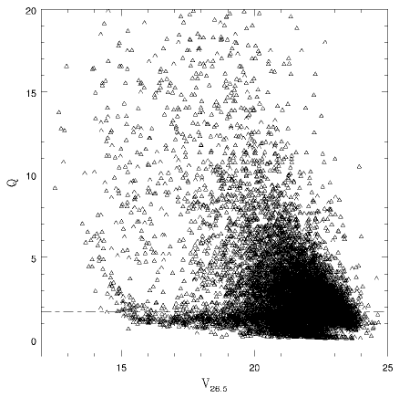
Figure 2: Normalized compactness parameter Q vs. isophotal magnitude for all observed objects. The dashed line indicates the Q_sep = 1.7 value determined to separate stars (below the line) from galaxies (above the line).

Figure 3: Histogram of magnitudes for raw galaxy counts. The turnover of the histogram, around V${}_{26.5}\sim 22.5$, gives an estimate of the completeness magnitude of the observations. Poisson error bars are displayed.

A pitfall of this classification procedure could be the misclassification of compact galaxies as stars. In order to test the reliability of the separation, we carried out a simple test. After having transformed our CCD coordinates into the GMP reference system (see section 5), we identified our objects with those belonging to the Coma redshift catalogue obtained by Biviano et al. (1995). We thus estimated that, out of 278 identifications, less than 2 $\%$ of the objects classified as galaxies by our procedure actually had star-like velocities.

It is obvious that this test is limited to a small number of identifications, since we can only apply it to objects with V $>$ 15, due to saturation, and V $\la$ 17, which is the 95 $\%$ completeness limit of the redshift catalogue. Nevertheless, it gives a representative result for the whole sample and reassures us on the efficiency and accurateness of the distinguishing procedure.

After elimination of repeated detections of some of the objects (see section 5) we ended up with a catalogue containing 7023 galaxies and 4096 stars.

4.4 Surface brightness selection effects

In order to test the detection limit of our observations imposed by the surface brightness we plot $\mu_{0}$ vs. V in Fig. 4. In this plot the diagonal cut shows the sequence of compact objects. Practically all objects below completeness magnitude 22.5 are placed at $\mu_{0}$ $\la$ 24.5 mag/arcsec², as confirmed by the turnover value of the histogram of $\mu_{0}$. Above that value detections are sparse. This limiting detection value might make us miss some very faint surface brightness objects, but below it we estimate our catalogue to be complete in surface brightness.

Figure 4: Central surface brightness plotted against isophotal magnitudes for all the catalogued galaxies. The dashed line indicates the completeness magnitude limit.

4.5 Zero point accuracy and errors estimated for the photometry derived parameters

The estimate of magnitude errors is done frame by frame, according to the variations detected in the sky flux for each exposure. By doing so we are certain of estimating a total error that includes both internal errors inherent to the measurement algorithm, as well as external errors produced by the observational conditions such as differential absorption in the different nights of the run. We compute, for all of the objects in a given frame, a typical measure of the magnitude error that is given by :

$$|dV|=-2.5~{}log~{}(flux)+2.5~{}log~{}(flux+\sigma)$$ (2)

where the first term of the right-hand side of the equation is the magnitude in the catalogue. In the second term, $\sigma$ has been computed by averaging, for each frame, different values of the standard deviation of the sky flux measured in different regions devoid of objects in that frame, and scaling the result to the surface of each object. The errors introduced by the flat–field procedure (large scale residuals) are less than 0.3$\%$, and this factor was neglected in the standard deviation estimation of the flux measurement.
In Fig. 5 we plot $|dV|$ vs. V for all the objects individually (upper pannel) and its mean value and dispersion per magnitude bin in the lower pannel. The mean value is below 0.1 magnitude.

Figure 5: Magnitude total errors for all catalogued objects computed by means of equation 2 (upper panel). We also show, per magnitude bin, the mean error and dispersion (lower panel).

Another point we set out to deal with in this section - zero point variations - is tackled by means of the 1082 galaxies with V brighter than the completeness magnitude value that were measured twice in the overlapping CCD areas (see section 5). Fig. 6 displays magnitudes for these objects. The points cluster closely around the quadrant line y=x with a larger dispersion for fainter magnitudes, as expected. One can notice that differences are not systematic. In Fig. 7 we quantify these results by computing, for each of the 1082 galaxies, the modulus of the difference between the magnitudes measured in two distinct frames (that is, the values plotted in the 2 axis of the previous figure). We also display, for each magnitude bin, the median and dispersion of those absolute differences for the objects belonging to that bin. Below completeness magnitude the median does not exceed 0.15 and one should bear in mind that this value comprises the magnitude errors (discussed above) for both measures. It is thus by far an overestimate of the zero point accuracy.

In what concerns $\mu_{0}$, errors range from 0.02 to 0.4 mag/arcsec² for bright to faint objects below the completeness magnitude limit.

5 Astrometry

We performed a standard transformation on our CCD coordinates to the reference system defined by Godwin et al. (1983, GMP). In this system each object has (X,Y) coordinates in arcsec, given relatively to a center defined at $\alpha=12^{h}57.3^{m},\delta=28^{o}14.4^{\prime}~{}(1950)$ - located between both largest/brightest central galaxies, NGC 4874 and NGC 4889 (see Fig. 1). For spectroscopic purposes, the frames were taken with a large superposition in Y (of the order of 40 $\%$, while almost negligible in X), which caused double observation of many objects. We carefully eliminated these double entries, both for stars and galaxies. In order to estimate the final precision of our positions, we compared our star catalogue with the Guide Star Catalogue (GSC) of the Hubble Space Telescope limited to magnitude m$<$15.5, which has a 0.3 arcsec accuracy. The positions of the same objects in both catalogues coincided, after final tuning, within less than 3 arcsec (median result for 17 stars identified in the field of our observations).

6 The catalogue

The catalogue, available in electronic form alone at the CDS (Centre de Données Astronomiques de Strasbourg), presents the following entries for all objects in both regions of observation (the large central zone and the smaller south-west area - see Fig. 1) :
(1,2,3) Right ascension (1950).
(4,5,6) Declination (1950).
(7) Isophotal radius r_26.5 in arcsec.
(8) Central surface brightness $\mu_{0}$ in mag/arcsec².
(9) Isophotal apparent magnitude V_26.5.
(10) Magnitude error (in modulus), as estimated by equation 2.
(11) Classification of the object : 1 $=$ star, 0 $=$ galaxy.
(12) GMP number, when available. The letter after the number indicates the GMP catalogue used for the matching : g stands for the GMP (1983) galaxy catalogue, while s stands for the GMP unpublished star catalogue. The correspondance was obtained by cross-correlating positions. Do notice there are inevitable ambiguities in this cross-identification, possibly due to non resolution of close objects by GMP or simply to confusion when several close neighbours exist. That is why there are 4 entries doubled (because each one of those 4 objects was identified with 2 different GMP objects : 3325g, 3336g, 2976g, 2980g, 4068g, 4075g and 4032s, 4042s). In addition, there are also several other entries which are attributed the same GMP number. We thus caution the reader/potential user of this catalogue to beware not to use these data directly without taking into account this information.
(13,14) GMP (X,Y) coordinates in arcsec (after slight correction to match GSC positions, as described in section 5).
(15) Heliocentric radial velocity in km s^-1, when available, as given by Biviano et al. (1995).

Figure 6: Galaxies measured twice : for each one we compare its magnitude as obtained in two different frames.

Figure 7: Crosses give the modulus of the difference between both magnitudes plotted in Fig. 6, for each one of the double measured galaxies, as a function of the galaxy’s magnitude as measured in one of the frames. Circles stand for the median value of this difference in each magnitude bin, and error bars show the dispersion around that median.

Some of the results derived from the analysis of this catalogue are discussed in Lobo et al. 1996 (in press), Gerbal et al. 1996 (submitted) and the corresponding available spectral data is published by Biviano et al. (1995).

- [1] Biviano A., Durret F., Gerbal D. et al., 1995, AAS 111, 265
- [2] Christian C.A., Adams M., Barnes J.V. et al., 1985, PASP 977, 363
- [3] Gerbal D., Lima-Neto G., Márquez I., Verhagen H., 1996, MNRAS, in preparation
- [4] Godwin J.G., Metcalfe N., Peach J.V., 1983, MNRAS 202, 113 (GMP)
- [5] Le Fèvre O., Bijaoui A., Mathez G., Picat J.P., Lelièvre G., 1986, A&A 154, 92
- [6] Le Fèvre O., Crampton D., Felenbok P., Monnet G., 1994, A&A 282, 325
- [7] Lilly S.J., Le Fèvre O., Crampton D., Hammer F., Tresse L., 1995, ApJ 455, 50
- [8] Lobo C., Biviano A., Durret F. et al., 1996, AA, in press
- [9] Slezak E., Bijaoui A., Mars G., 1988, A&A 201, 9