MEASURING POLARIZATION IN THE COSMIC MICROWAVE BACKGROUND

Abstract

Polarization induced by cosmological scalar perturbations leads to a typical anisotropy pattern, which can best be analyzed in Fourier domain. This allows one to unambiguously distinguish cosmological signal of polarization from other foregrounds and systematics, as well as from polarization induced by non-scalar perturbations. The precision with which polarization and cross-correlation power spectra can be determined is limited by cosmic variance, noise and foreground residuals. Choice of estimator can significantly improve our capability of extracting cosmological signal and in the noise dominated limit the optimal power spectrum estimator reduces the variance by a factor of two compared to the simplest estimator. If foreground residuals are important then a different estimator can be used, which eliminates systematic effects from foregrounds so that no further foreground subtraction is needed. A particular combination of Stokes $Q$ and $U$ parameters vanishes for scalar induced polarization, thereby allowing an unambiguous determination of tensor modes. Theoretical predictions of polarization in standard models show that one typically expects a signal at the level of 5-10$\mu$K on small angular scales and around 1$\mu$K on large scales ($l<200$). Satellite missions should be able to reach sensitivities needed for an unambiguous detection of polarization, which would help to break the degeneracies in the determination of some of the cosmological parameters.

1 Introduction

Anisotropies in cosmic microwave background (CMB) are now widely accepted as the best probe of early universe, which can potentially provide information over a whole range of cosmological parameters (Jungman et al. 1996; Zaldarriaga, Spergel & Seljak 1996). The main advantage of CMB anisotropies as opposed to other, more local probes, is that they are sensitive to the universe in the linear regime, which statistical properties can easily be calculated starting from ab-initio theoretical models and compared to the observations. A dozen or so cosmological parameters could be extracted from the observations produced by the future satellite and ground based experiments. There are two potential problems in this program. First is the somewhat uncertain amount of galactic and extragalactic foregrounds, which could severely limit our ability to extract cosmological signal from the data. Second is the degeneracies among some of the cosmological parameters, which allows only certain combinations to be determined accurately, but does not allow to break the degeneracies between them (Bond et al. 1995; Jungman et al. 1996; Zaldarriaga et al. 1996).

It is therefore important to investigate other independent confirmations of results produced from CMB anisotropies and it has long been recognized that polarization in the microwave sky might provide such an independent test (Rees 1968, Polnarev 1985, Bond & Efstathiou 1987, Crittenden, Davis & Steinhardt 1993, Frewin, Polnarev & Coles 1994, Coulson, Crittenden & Turok 1994, Crittenden, Coulson & Turok 1995). Like temperature anisotropy, polarization probes the universe in the linear regime and so can provide information useful to determine cosmological parameters. It is specially important for determining parameters which are only weakly constrained by the CMB anisotropies alone, such as the epoch of reionization or the presence of tensor perturbations. In both of these cosmic variance is the limiting factor in our capability of extracting the parameters, so measuring polarization would increase the amount of information and allow for a more accurate determination of the parameters. Both polarization-polarization and polarization-temperature correlation give an independent set of power spectra, which have different sensitivity to different parameters, so combining them results in a much larger information about the underlying cosmological model and can significantly increase our capability of extracting useful information from the CMB measurements.

The main disadvantage of polarization is that it is predicted to be of a rather low amplitude, of the order of 10% of temperature anisotropy, so measuring it represents an experimental challenge that has yet to be overcome. Currently there are no positive detections of polarization, with the best upper limits of the order of $25\mu K$ (Wollack et al. 1993). This situation needs not continue in the future, however, as the experimental sensitivity increases and new larger and better experiments are being planned. Moreover, as shown in this paper, cosmologically induced polarization has a unique signature in the data that cannot be mimicked by other foregrounds and provides a clear test of the searched signal. An experiment at Brown (Timbie 1996) plans to reach sensitivities of a few $\mu K$, which should be sufficient to detect the polarization signal if our current expectations are correct. Interferometer observations could be able to extend this to much larger areas of the sky and produce maps of polarization both in real space and in frequency space. Unfortunately, at present none of the planned interferometer experiments is including polarization, although as argued in this paper frequency space has many advantages in search for the unique signature of cosmological polarization. Finally, all sky satellite maps of polarization are also planned by MAP and COBRAS/SAMBA satellites and may eventually provide us with very high accuracy maps of polarization pattern in the sky.

The outline of this paper is the following. In §2 statistical properties of polarization parameters are derived in the small scale limit. Special nature of polarization induced by scalar perturbations allows one to use statistical methods developed in the context of weak lensing (Kaiser 1992). In §3 various 2-point estimators are presented both in Fourier and real space, together with their variances and covariances. §4 is devoted to the foregrounds and possible methods of their elimination. Polarization induced by tensor modes is discussed in §5 and the difference between the two types of perturbations is highlighted. In §6 theoretical predictions for polarization are computed for a variety of cosmological models and the ability to extract them with the satellite missions is discussed. This is followed by conclusions in §7.

2 Polarization in the small scale limit

In this section we derive the small-scale limit of temperature and polarization anisotropies. This limit is of special interest, because one can replace the general spherical expansion with the Fourier expansion and the expressions simplify considerably. The analysis in this section will be restricted to polarization generated by scalar perturbations. Tensor perturbations are discussed in §5.

In general one can describe CMB polarization as a 2x2 temperature perturbation tensor $T_{ij}$. Stokes parameters $Q$ and $U$ (we will ignore $V$ in the following, since it cannot be generated through Thomson scattering) are defined as $Q=T_{xx}-T_{yy}$ and $U=2T_{xy}=2T_{yx}$, while temperature anisotropy is just its trace, $T=T_{xx}+T_{yy}$. The components are defined with respect to a fixed coordinate system $(x,y)$ perpendicular to the photon direction $\vec{n}$. The Stokes parameter $Q$ is positive if temperature perturbation is larger along the $x$ relative to the $y$ axis, while $U$ parameter is positive if perturbation is larger along the upper right diagonal relative to the upper left diagonal.

Equations of radiative transfer for polarization and temperature anisotropy simplify in Fourier space if we work in a frame with the axis defined parallel and perpendicular to $\partial/\partial\beta$, where $\beta$ is the angle between the wavevector $\vec{k}$ and photon direction $\vec{n}$. Azimuthal symmetry guarantees that the Thomson scattering preserves the diagonal form of $I_{ij}$, just like in the case of plane-parallel atmospheres (Chandrasekhar 1960, Kaiser 1983). In terms of the Stokes parameters only $Q$ is excited in this frame. This puts a restriction on the general form of polarization and as we show below it can be used to separate cosmologically induced polarization from other sources and systematic effects. Although only $Q$ is present in this frame, when we rotate polarization by an azimuthal angle $-\phi_{\vec{k},\vec{n}}$ to a fixed frame in the sky we generate both $Q$ and $U$. At the observers position the expressions for $T$, $Q$ and $U$ are given by (Bond & Efstathiou 1987, Kosowsky 1996),

$$T(\vec{n}) = \int d^{3}\vec{k}\Delta_{T}(\vec{k},\vec{n})$$

$$Q(\vec{n}) = \int d^{3}\vec{k}\Delta_{P}(\vec{k},\vec{n})\cos(2\phi_{\vec{k},\vec{n}})$$

$$U(\vec{n}) = \int d^{3}\vec{k}\Delta_{P}(\vec{k},\vec{n})\sin(2\phi_{\vec{k},\vec{n}}),$$ (1)

where $\Delta_{T,P}(\vec{k},\vec{n})$ are the Fourier components of temperature and polarization distribution function integrated over the momentum and $\vec{n}$ is the direction of observation on the sky. The expression for rotation angle $\phi_{\vec{k},\vec{n}}$ depends both on $\vec{k}$ and $\vec{n}$, but if we restrict our attention to the directions $\vec{n}$ around the pole then it can be approximated with $-\phi_{k}$, where $\phi_{k}$ is the azimuthal angle of vector $\vec{k}$. This approximation breaks down for wavemodes $\vec{k}$ close to the pole ($\hat{z}$ direction), but for sufficiently small scales the contribution from these modes to the total power becomes negligible.

The solution for $\Delta_{T,P}(\vec{k},\vec{n})$ can be written as an integral over the sources along the line of sight (Seljak & Zaldarriaga 1996)

$$\Delta_{T,P}(\vec{k},\vec{n})=\int_{0}^{\tau_{0}}d\tau e^{i\vec{k}\cdot\vec{n}(\tau-\tau_{0})}S_{T,P}(k,\tau),$$ (2)

where $S_{T,P}(k,\tau)$ are the source functions for temperature and polarization and can be expressed in terms of metric, baryon and photon perturbations (see Seljak & Zaldarriaga 1996 for their explicit expressions). By combining equations 1 and 2 we can write the complete solutions for $T(\vec{n})$, $Q(\vec{n})$ and $U(\vec{n})$. The only term that depends on the direction $\vec{n}$ in equation 2 is the exponential. The expressions for polarization can therefore be simplified by noting that for the directions $\vec{n}$ near the pole $\cos(2\phi_{\vec{k}})$ and $\sin(2\phi_{\vec{k}})$ can be written in terms of second derivatives with respect to $\vec{\theta}$, the 2-dimensional projection of $\vec{n}$ onto fixed $(x,y)$ plane perpendicular to the pole. This leads to

$$Q(\vec{n}) = D_{Q}(\vec{n})\int d^{3}\vec{k}\Delta_{P}(\vec{k},\vec{n}),\,\,\,\,\,\,\,\,\,\,\,\,\,\,\,D_{Q}(\vec{n})=(\partial\theta_{x}\partial\theta_{x}-\partial\theta_{y}\partial\theta_{y})\nabla_{\theta}^{-2}$$

$$U(\vec{n}) = D_{U}(\vec{n})\int d^{3}\vec{k}\Delta_{P}(\vec{k},\vec{n}),\,\,\,\,\,\,\,\,\,\,\,\,\,\,\,D_{U}(\vec{n})=2\partial\theta_{x}\partial\theta_{y}\nabla_{\theta}^{-2},$$ (3)

where $\nabla_{\theta}^{-2}$ is the inverse 2-d Laplacian with respect to $\vec{\theta}$ and $\theta_{x}$, $\theta_{y}$ are the components of $\vec{\theta}$ in the fixed basis on the sky. Because $\Delta_{T,Pl}(\vec{k},\vec{n})$ depend only on the angle between the two vectors one can expand them in Legendre series,

$$\Delta_{T,P}(\vec{k},\vec{n})=\sum_{l}(2l+1)(-i)^{l}\Delta_{T,Pl}(k)P_{l}(\mu),$$ (4)

where $\mu=\vec{k}\cdot\vec{n}$. The rms values for $\Delta_{T,Pl}(k)$ can be obtained by solving the Boltzmann equation in differential form or the integral solution itself (Bond & Efstathiou 1987, Seljak & Zaldarriaga 1996).

Each of the observable quantities $T(\vec{n})$, $Q(\vec{n})$ and $U(\vec{n})$ can be expanded on a sphere into spherical harmonics or their derivatives,

$$T(\vec{n}) = \sum_{lm}a_{Tlm}Y_{lm}(\vec{n})$$

$$Q(\vec{n}) = \sum_{lm}a_{Plm}D_{Q}(\vec{n})Y_{lm}(\vec{n})$$

$$U(\vec{n}) = \sum_{lm}a_{Plm}D_{U}(\vec{n})Y_{lm}(\vec{n})$$

$$a_{T,Plm} = 4\pi(-i)^{l}\int d^{3}\vec{k}Y^{*}_{lm}(\vec{k})\Delta_{T,Pl}(\vec{k}).$$ (5)

The statistical properties of $a_{T,Plm}$ coefficients follow from equation 5 above,

$$\langle a_{Tlm}^{*}a_{Tl^{\prime}m^{\prime}}\rangle = \delta_{ll^{\prime}}\delta_{mm^{\prime}}\int d^{3}k\Delta^{2}_{Tl}(k)\equiv\delta_{ll^{\prime}}\delta_{mm^{\prime}}C_{Tl}$$

$$\langle a_{Plm}^{*}a_{Pl^{\prime}m^{\prime}}\rangle = \delta_{ll^{\prime}}\delta_{mm^{\prime}}\int d^{3}k\Delta^{2}_{Pl}(k)\equiv\delta_{ll^{\prime}}\delta_{mm^{\prime}}C_{Pl}$$ (6)

The cross-correlation between temperature and polarization is given by

$$\langle a_{Tlm}^{*}a_{Pl^{\prime}m^{\prime}}\rangle=\delta_{ll^{\prime}}\delta_{mm^{\prime}}\int d^{3}k\Delta_{Tl}(k)\Delta_{Pl}(k)\equiv\delta_{ll^{\prime}}\delta_{mm^{\prime}}C_{Cl}.$$ (7)

Because we are only interested in $\vec{n}$ near the pole one can approximate the sphere locally as a plane, in which case instead of spherical decomposition we may use plane wave expansion. In this limit we replace $\sum_{lm}a_{Plm}Y_{lm}(\vec{n})$ with $\int d^{2}\vec{l}P(\vec{l})e^{i\vec{l}\cdot\vec{\theta}}$ (and analogously for temperature anisotropy). Differential operators $D_{Q}(\vec{n})$ and $D_{U}(\vec{n})$ acting on $e^{i\vec{l}\cdot\vec{\theta}}$ become simple again and bring out $\cos(2\phi_{\vec{l}})$ and $\sin(2\phi_{\vec{l}})$, respectively, where $\phi_{\vec{l}}$ is the direction angle of 2-dimensional vector $\vec{l}$ with amplitude $l$. This leads to

$$T(\vec{\theta}) = (2\pi)^{-2}\int d^{2}\vec{l}e^{i\vec{l}\cdot\vec{\theta}}T(\vec{l})$$

$$Q(\vec{\theta}) = (2\pi)^{-2}\int d^{2}\vec{l}e^{i\vec{l}\cdot\vec{\theta}}P(\vec{l})\cos(2\phi_{\vec{l}})$$

$$U(\vec{\theta}) = (2\pi)^{-2}\int d^{2}\vec{l}e^{i\vec{l}\cdot\vec{\theta}}P(\vec{l})\sin(2\phi_{\vec{l}}).$$ (8)

$T(\vec{l})$ and $P(\vec{l})$ are the Fourier components of temperature anisotropy and polarization in $\vec{l}$ space and have the statistical properties,

$$\langle T(\vec{l})T^{*}(\vec{l^{\prime}})\rangle=(2\pi)^{2}C_{Tl}\delta_{D}(l-l^{\prime})$$

$$\langle P(\vec{l})P^{*}(\vec{l^{\prime}})\rangle=(2\pi)^{2}C_{Pl}\delta_{D}(l-l^{\prime})$$

$$\langle T(\vec{l})P^{*}(\vec{l^{\prime}})\rangle=(2\pi)^{2}C_{Cl}\delta_{D}(l-l^{\prime}),$$ (9)

where $\delta_{D}(l-l^{\prime})$ is the Dirac $\delta$ function as opposed to the Kronecker $\delta$ in the discrete case and $C_{l}$ is assumed to be a continuous function obtained by interpolation from the discrete spectrum defined in equation 7.

To generate a map of temperature anisotropy and polarization one proceeds in the following way. For each pair of vectors $\vec{l}$, $-\vec{l}$ on a discrete mesh one diagonalizes the correlation matrix $M_{11}=C_{Tl}$, $M_{22}=C_{Pl}$, $M_{12}=M_{21}=C_{Cl}$, where $l$ is the amplitude of vector $\vec{l}$. One then generates from a normalized gaussian distribution two pairs of random numbers and multiplies them with the amplitudes given by the square root of the correlation matrix eigenvalues. Rotating this vector pair back to the original frame gives a realization of $T(\vec{l})$ and $P(\vec{l})$ (and their complex conjugates corresponding to $-\vec{l}$), from which follow $Q(\vec{l})=P(\vec{l})\cos(2\phi_{\vec{l}})$ and $U(\vec{l})=P(\vec{l})\sin(2\phi_{\vec{l}})$. Fourier transform of $T$, $Q$ and $U$ back into the real space gives a map of these quantities in the sky in the small-scale limit, with the correct auto and cross correlations among all the quantities. Note that this differs from the prescription given in Bond & Efstathiou 1987.

3 2-point estimators

The 2-point correlations can be calculated either in angular or in frequency (Fourier) space. While the two are related via a Fourier transform, there are certain advantages to the analysis performed in frequency space. In the first subsection we explore this approach, while the correlation function approach and the comparison between the two are explored in the next subsection.

3.1 Power spectrum analysis

From a map of $T(\vec{\theta})$, $Q(\vec{\theta})$ and $U(\vec{\theta})$ we can obtain their analogs in frequency space by Fourier transform, $X(\vec{l})=\int d^{2}\vec{\theta}e^{-i\vec{l}\cdot\vec{\theta}}X(\vec{\theta})$, where $X$ stands for $T$, $Q$ or $U$. Using the expressions given in the previous section one obtains the two-point functions of these quantities,

$$\langle T(\vec{l})T^{*}(\vec{l^{\prime}})\rangle = (2\pi)^{2}C_{Tl}\delta_{D}(l-l^{\prime})$$

$$\langle T(\vec{l})Q^{*}(\vec{l^{\prime}})\rangle = (2\pi)^{2}C_{Cl}\cos(2\phi_{\vec{l}})\delta_{D}(l-l^{\prime})$$

$$\langle T(\vec{l})U^{*}(\vec{l^{\prime}})\rangle = (2\pi)^{2}C_{Cl}\sin(2\phi_{\vec{l}})\delta_{D}(l-l^{\prime})$$

$$\langle Q(\vec{l})Q^{*}(\vec{l^{\prime}})\rangle = (2\pi)^{2}C_{Pl}\cos^{2}(2\phi_{\vec{l}})\delta_{D}(l-l^{\prime})$$

$$\langle U(\vec{l})U^{*}(\vec{l^{\prime}})\rangle = (2\pi)^{2}C_{Pl}\sin^{2}(2\phi_{\vec{l}})\delta_{D}(l-l^{\prime}).$$ (10)

We see that the correlations in polarization give rise to a very characteristic anisotropy pattern in $\vec{l}$ space. This arises from the fact that polarization was not generated from a general mechanism, but rather through a process of Thomson scattering, which cannot generate $U$ and $V$ components in the $\vec{k}$ dependent frame defined in previous section. This characteristic anisotropy can therefore be used to separate true signal from instrumental artifacts and foregrounds, which is discussed in more detail in next section. Alternatively, if foregrounds can be kept under control one can use the characteristic anisotropy to separate scalar induced polarization from the one induced by vector or tensor modes, which do not obey the same anisotropy pattern (§5).

To estimate the sensitivity that is possible to achieve in a measurement of polarization power spectrum let us assume the measurements are given on a square grid of $N$ pixels with a total solid angle $\Omega$. The antenna beam smearing will be described with $b(l)$. In the case of single dish observations with a gaussian beam this is given by $b(l)=e^{l^{2}\sigma_{b}^{2}/2}$, where $\sigma_{b}$ is the gaussian size of the beam. In the case of interferometers $b(l)$ is either 1 or 0, depending on whether the particular frequency is observed or not. We will assume that different measurements are uncorrelated by taking mesh spacing large enough to ignore correlations induced by finite window (Hobson & Magueijo 1996). In the case of single dish experiments each pixel in real space has a noise contribution with rms noise amplitudes $\sigma_{T}$, $\sigma_{P}$ for temperature and both components of polarization, respectively (we assume for simplicity that $Q$ and $U$ are being measured equal amounts of time). We will also assume that noise is uncorrelated between different pixels and between different polarization components $Q$ and $U$. This is only the simplest possible choice and more complicated noise correlations arise if all the components are obtained from a single set of observations. In the case of Brown polarization experiment (Timbie 1996) the polarization measurements will be made by rotating the antenna axis by $45^{\circ}$, each time measuring directly the difference between the two orthogonal polarizations. This would therefore provide a direct measurement of $Q$ and $U$ components with no noise mixing between them. In the case of interferometers each pixel in $\vec{l}$ space is measured directly and the noise is uncorrelated between individual pixels in frequency space. Following Knox 1995 we will introduce pixel independent measure of noise $w^{-1}_{T,P}=\Omega\sigma^{2}_{T,P}/N$ for single dish experiments and $w^{-1}_{T,P}=\sigma^{2}_{T,P}$ for interferometers (see Hobson & Magueijo 1996 for expressions that relate $\sigma_{T,P}$ to the receiver sensitivity). For cross-correlation between temperature and polarization there are two simple cases to be considered. In one the cross-correlation is being made with two different maps, in which case noise is uncorrelated. In the second case both temperature and polarization are obtained from the same experiment by adding and differenciating the two polarization states. In this case noise in temperature and polarization are related via $\sigma_{T}^{2}=\sigma_{P}^{2}/2$. In both cases noise in temperature is uncorrelated with noise in polarization components, so the final expressions are identical.

The first step is to construct a discrete Fourier transform of the map, $\hat{X}(\vec{l})=N^{-1}\sum e^{-i\vec{l}\cdot\vec{\theta}}X(\vec{\theta})$. Using the observed quantities $\hat{T}(\vec{l})$, $\hat{Q}(\vec{l})$ and $\hat{U}(\vec{l})$ we can form power spectrum estimates. The simplest one is for temperature anisotropy, which for single dish observations is given by

$$\hat{C}_{Tl}=\left[\sum_{l}{\Omega\over N_{l}}[\hat{T}(\vec{l})\hat{T}^{*}(\vec{l})]-w^{-1}_{T}\right]b^{-2}(l),$$ (11)

where the term $b^{-2}(l)$ accounts for beam smearing and $N_{l}$ is the number of independent modes around $l$. The expression for interferometers is the same without the beam smearing term and summing only over the observed modes in frequency space. We will only present expressions for single dish here, as the modification for interferometers is obvious. Each mode $\hat{T}(\vec{l})$ is a complex random variable with 0 mean and variance $C_{Tl}b^{2}(l)+w^{-1}_{T}$. The variance on estimator $\hat{C}_{Tl}$ for a single pair of modes $\hat{T}(\vec{l})$, $\hat{T}(-\vec{l})$ is therefore $C_{Tl}b^{2}(l)+w^{-1}_{T}$. If we average over $N_{l}$ modes the variance is reduced by $N_{l}^{-1/2}$. There are $l^{2}\Omega d\ln l/2\pi$ modes of amplitude $l$ in an interval $d\ln l$, which leads to the variance

$${\rm Cov}(C_{Tl}^{2})=C_{Tl}^{2}{4\pi\over l^{2}\Omega d\ln l}\left(1+[w_{T}C_{Tl}b^{2}(l)]^{-1}\right)^{2},$$ (12)

where ${\rm Cov}(XX^{\prime})\equiv\langle(\hat{X}-\langle\hat{X}\rangle)(\hat{X}^{\prime}-\langle\hat{X}^{\prime}\rangle)\rangle$. If there is more than one field the variance decreases inversely proportional to the square root of number of fields (Hobson & Magueijo 1996). In the limit of large sky coverage it reduces to the expressions given by Knox 1995 and Jungman et al. 1996.

In the case of polarization there are several estimators that one can form. The simplest one is given by

$$\hat{C}_{Pl}=\left[{\Omega\over N_{l}}\sum_{l}[\hat{Q}(\vec{l})\hat{Q}^{*}(\vec{l})+\hat{U}(\vec{l})\hat{U}^{*}(\vec{l})]-2w^{-1}_{P}\right]b^{-2}(l),$$ (13)

The single mode pair variance for this estimator is $(C_{Pl}^{2}b^{4}(l)+2C_{Pl}b^{2}(l)w^{-1}_{P}+4w^{-2}_{P})^{1/2}$. If noise is dominant contributor to the variance, as it is likely to be the case for polarization given the small overall amplitude of the signal, then this estimator is far from optimal. The optimal estimator is

$$\hat{C}_{Pl}=\left[{\Omega\over N_{l}}\sum_{l}|\hat{Q}(\vec{l})\cos(2\phi_{\vec{l}})+\hat{U}(\vec{l})\sin(2\phi_{\vec{l}})|^{2}-w^{-1}_{P}\right]b^{-2}(l),$$ (14)

which has single mode pair variance $C_{l}b^{2}(l)+w^{-1}_{P}$. In the limit of noise dominated variance this is 2 times smaller than the variance of the estimator in equation 13. Averaging over all modes in $d\ln l$ gives

$${\rm Cov}(C_{Pl}^{2})=C^{2}_{Pl}{4\pi\over l^{2}\Omega d\ln l}\left(1+[w_{P}C_{Pl}b^{2}(l)]^{-1}\right)^{2}.$$ (15)

Finally, for cross-correlation the optimal estimator is,

$$\hat{C}_{Cl}={\Omega\over 2N_{l}}\sum_{l}\left[\left(\hat{Q}(\vec{l})\hat{T}^{*}(\vec{l})+\hat{Q}^{*}(\vec{l})\hat{T}(\vec{l})\right)\cos(2\phi_{\vec{l}})+\left(\hat{U}(\vec{l})\hat{T}^{*}(\vec{l})+\hat{U}^{*}(\vec{l})\hat{T}(\vec{l})\right)\sin(2\phi_{\vec{l}})\right]b^{-2}(l),$$ (16)

which has a single mode pair variance $[(C^{2}_{Cl}b^{4}(l)+(C_{Tl}b^{2}(l)+w_{T}^{-1})(C_{Pl}b^{2}(l)+w_{P}^{-1}))/2]^{1/2}$. As before, averaging over the modes reduces this variance inversely proportional to the square root of the number of modes and gives,

$${\rm Cov}(C_{Cl}^{2})=C^{2}_{Cl}{2\pi\over l^{2}\Omega d\ln l}\left[1+{(C_{Tl}b^{2}(l)+w_{T}^{-1})(C_{Pl}b^{2}(l)+w_{P}^{-1})\over C^{2}_{Cl}b^{4}(l)}\right].$$ (17)

For a study of cosmological parameters one also needs to include the covariance elements between various power spectrum estimators. These are given by

$${\rm Cov}(C_{Tl}C_{Pl}) = C_{Cl}^{2}(l){4\pi\over l^{2}\Omega d\ln l}$$

$${\rm Cov}(C_{Cl}C_{Tl}) = C_{Cl}C_{Tl}{4\pi\over l^{2}\Omega d\ln l}(1+[w_{T}C_{Tl}b^{2}(l)]^{-1})$$

$${\rm Cov}(C_{Cl}C_{Pl}) = C_{Cl}C_{Pl}{4\pi\over l^{2}\Omega d\ln l}(1+[w_{P}C_{Pl}b^{2}(l)]^{-1}).$$ (18)

3.2 Correlation function analysis

In this subsection we explore the correlation function analysis of CMB anisotropies. Taking Fourier transform of the power spectra leads to the following correlation functions,

$$\langle T(0)T(\vec{\theta})\rangle = \int{ldl\over 2\pi}C_{Tl}b^{2}(l)J_{0}(l\theta)$$

$$\langle Q(0)Q(\vec{\theta})\rangle = \int{ldl\over 4\pi}C_{Pl}b^{2}(l)[J_{0}(l\theta)+\cos(4\phi)J_{4}(l\theta)]$$

$$\langle U(0)U(\vec{\theta})\rangle = \int{ldl\over 4\pi}C_{Pl}b^{2}(l)[J_{0}(l\theta)-\cos(4\phi)J_{4}(l\theta)]$$

$$\langle Q(0)U(\vec{\theta})\rangle = \int{ldl\over 4\pi}C_{Pl}b^{2}(l)\sin(4\phi)J_{4}(l\theta)$$

$$\langle T(0)Q(\vec{\theta})\rangle = \int{ldl\over 4\pi}C_{Cl}b^{2}(l)\cos(2\phi)J_{2}(l\theta)$$

$$\langle T(0)U(\vec{\theta})\rangle = \int{ldl\over 4\pi}C_{Cl}b^{2}(l)\sin(2\phi)J_{2}(l\theta),$$ (19)

where $\phi$ is the direction angle of $\vec{\theta}$ and $J_{n}(x)$ are the Bessel functions of order $n$. Although the characteristic anisotropy is present also in the correlation functions, it is more complicated, because there are actually two independent correlation functions for polarization,

$$C^{1}_{P}(\theta) = \int{ldl\over 4\pi}C_{Pl}b^{2}(l)J_{0}(l\theta)$$

$$C^{2}_{P}(\theta) = \int{ldl\over 4\pi}C_{Pl}b^{2}(l)J_{4}(l\theta),$$ (20)

both of which of course depend on the same underlying power spectrum. Moreover, the prior $C_{Pl}>0$ becomes a set of integral constraints in real space, which is more difficult to impose on the estimators obtained from the data. All this argues for Fourier space analysis as the method of choice in the case of polarization.

Expressions above agree with those derived by Coulson et al. 1994 and Kosowsky 1996, which for $QQ$ and $UU$ are also only valid in the small scale limit, but where this limit has not been consistently applied to all the steps, so that their final expressions look much more complicated than they actually are. They contain a term involving double summation over $\Delta_{Pl}$, $\Delta_{Pl^{\prime}}$ in the $\phi$ dependent term, which as shown in Appendix reduces to the expressions above if one consistently applies small scale limit to their expression. All the information about polarization is therefore contained in $C_{Pl}$ and $C_{Cl}$. Note that taking the Fourier transform of $QQ$ or $UU$ correlation function does not result in the power spectrum of $C_{Pl}$, but has an additional $\phi$ dependent term that involves a double integral of $J_{0}(l\theta)$ and $J_{4}(l^{\prime}\theta)$ over $l^{\prime}$ and $\theta$. Although generally smaller than $C_{Pl}$, this integral does not vanish in general, hence the appearance of such terms in expressions by Coulson et al. (1994) and Kosowsky (1996). This is of course not the optimal way to obtain the power spectrum from the correlation function. To obtain an estimate of the underlying power spectrum it is better to work in the Fourier domain directly, following the methods given in previous subsection.

3.3 Predicting polarization from temperature maps

One can use the measured temperature maps to predict the polarization pattern. The estimator is

$$\hat{Q}(\vec{l})=\alpha T(\vec{l})\cos(2\phi_{\vec{l}}),\,\,\,\,\hat{U}(\vec{l})=\alpha T(\vec{l})\sin(2\phi_{\vec{l}}),$$ (21)

where by minimizing the variance

$$\langle[\hat{Q}(\vec{l})-Q(\vec{l})]^{2}\rangle=\cos^{2}(2\phi_{\vec{l}})[\alpha^{2}C_{Tl}-2\alpha C_{Cl}+C_{Pl}]$$ (22)

and similarly for $U$ one finds $\alpha=C_{Cl}/C_{Tl}$, so that the fractional variance in the estimator is

$${\langle[\hat{Q}(\vec{l})-Q(\vec{l})]^{2}\rangle\over Q(\vec{l})^{2}}=1-\rm{Corr}(T,P)_{l}^{2}.$$ (23)

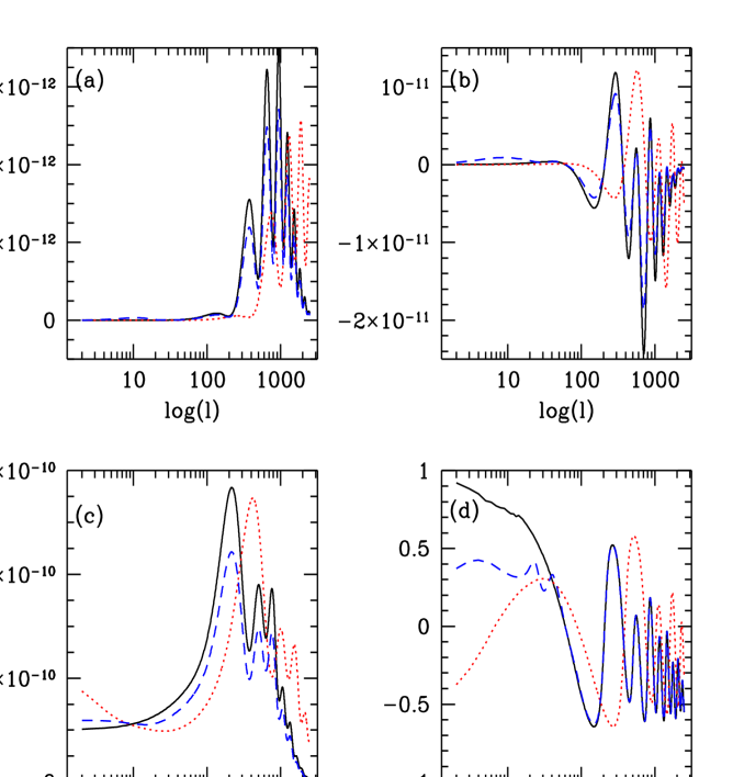
Figure 1: Power spectra of polarization (a), temperature-polarization cross correlation (b), temperature (c) and correlation coefficient (d). The models are standard CDM (solid curve), open CDM (dotted curve) and reionized standard CDM with optical depth of 0.2 (dashed curve).

The correlation coefficient is defined as $\rm{Corr}(T,P)_{l}=C_{Cl}/(C_{Tl}C_{Pl})^{1/2}$. Figure 1d shows that the correlation coefficient typically ranges between $-0.5$ and $0.5$ and so the fractional variance will be at best around 0.8 or so in $\vec{l}$ space and even larger than that in real space, where one averages over positive and negative cross-correlations in power spectrum. This is not very impressive in terms of predicting where to look for large polarization amplitude, although in a statistical sense one is still much more likely to find a high signal at a high $\sigma$ peak in the temperature map than at a random point (Coulson et al. 1994). On large angular scales ($l<10$) the correlation coefficient can be much larger and approaches unity in some models, so that the expressions in this limit would actually give a good correspondence between observed and predicted polarization. Unfortunately, the amplitude of polarization is extremely small on these scales and there is little hope to measure it in the near future even with the help of this “matching filter” technique.

4 Removal of foregrounds and other systematics

Although several galactic and extragalactic foregrounds are significant in the case of temperature measurements, only few of these are polarized and need to be considered for polarization measurements. Radiation from earth atmosphere and bremsstrahlung emission are not polarized at millimeter wavelengths and need not be discussed further (although atmospheric emission does have an effect by increasing the effective temperature of receiver and adding a fluctuating offset).

Extragalactic radio sources have synchrotron radiation as the dominant emission mechanism and can be 20% polarized. Their contribution to the polarization signal will be similar as their contribution to the temperature anisotropy signal and so analysis of point source effects on CMB can be directly applied to the case of polarization as well. This is discussed in more detail by Francheschini et al. (1989, 1991) and Tegmark & Efstathiou (1996). Point source contamination depends on the observed frequency, angular scale and flux cut above which point sources can be identified and eliminated. Poisson distribution produces a white-noise spectrum and at large angular scales radio point sources do not pose a significant problem. For example, on angular scales above $1^{\circ}$ their contribution is less than $1\mu K$ at 30 GHz (Timbie 1996), which is below the expected amplitude of the signal and is even less than that at higher frequencies. On smaller angular scales point sources become more important and more ambitious flux cuts are needed, which limits the area of the sky that can be observed. While in the case of temperature anisotropy this can be the main limitation of an experiment (and indeed of the whole CMB field), in the case of polarization we do have an additional constraint that allows us to separate cosmologically induced signal from the foregrounds. This is discussed in more detail below.

On large angular scales the main foreground contribution comes from our galaxy, where both dust and synchrotron emission can be polarized. Dust emission in the far-infrared is polarized up to 10% (Hildebrand et al. 1995). The contribution of dust to the lower frequency channels (where most HEMT based polarization measurements are being planned) is small. At frequencies below 100 Ghz the most important source of polarization is likely to be galactic synchrotron emission. Its linear polarization can reach 70%, so that polarization amplitudes of 50$\mu$K are expected around 30GHz (Cortiglioni & Spoelstra 1995). This drops significantly at higher frequencies and only a few $\mu$K synchrotron contamination in polarization is expected around 100GHz (Timbie 1996). Nevertheless, this is of the same order as the expected signal, so that some further foreground rejection is needed. One possibility is to use only clean parts of the sky where synchrotron emission is low, such as at high galactic latitudes. In addition, multifrequency CMB observations can be used to remove the foregrounds, which in the case of only one important foreground with approximately known frequency dependence can be very effective (Brandt et al. 1994). Accuracy of 1$\mu$K can be achieved with only two frequency channels if the noise level is around 1$\mu$K per pixel (Timbie 1996). Another possibility is multifrequency removal using the more sensitive temperature maps. This would be a useful strategy for example in the case of COBRAS/SAMBA satellite, where only lower frequency channels will have polarization capabilities, but all frequency channels could be used to determine the local contribution of various foregrounds. This way one could effectively remove multicomponent foregrounds from polarization even if only a few channels actually measured it.

While each of the foregrounds above can in principle be removed from the data, in practice this may not always be possible at the levels of 1$\mu$K and it would be useful to have an additional test of the presence of cosmological signal. Characteristic anisotropy of polarization in Fourier space provides such a test and gives a unique signature of polarization induced by scalar perturbations. To test whether the signal is cosmological one needs to compare the quantities

$$E(\vec{l})=Q(\vec{l})\cos(2\phi_{\vec{l}})+U(\vec{l})\sin(2\phi_{\vec{l}})$$ (24)

and

$$B(\vec{l})=-Q(\vec{l})\sin(2\phi_{\vec{l}})+U(\vec{l})\cos(2\phi_{\vec{l}}).$$ (25)

The first quantity contains all the polarization signal and its estimator is given in equation 14, while the second quantity vanishes even in the presence of cosmological polarization induced by scalar perturbations. This is true not just statistically, but for each Fourier mode individually. Most of the foregrounds should contribute on average the same amount to both variables. This is certainly valid for uncorrelated point sources, but even in the case of synchrotron and dust emission the alignment is preferentially determined by magnetic fields, which are not scalar in nature and will not exhibit the characteristic anisotropy in Fourier space. Hence the difference between $\hat{E}$ and $\hat{B}$ can be taken as a measure of the cosmological signal as compared to the foregrounds and/or instrumental offsets. If foregrounds and not noise are expected to be the main limitation then one may use may subtract the power spectrum of $\hat{E}$ from the one for $\hat{B}$ in equation 14 and no further foreground removal is needed. One could therefore use this technique to measure polarization even at frequencies below 50GHz, where foreground contribution is large, but could be averaged over if sufficient number of channels are being measured. Note that this test does not depend on the temperature anisotropies at all and can be applied directly to the measurements of $Q$ and $U$. To obtain a statistically significant measure of polarization one only needs to show that in an rms sense $\hat{E}$ is larger than $\hat{B}$. If one is noise and not foreground limited then it is more advantageous to use the optimal estimator in equation 14, because subtracting the power spectrum of $\hat{B}$ from the optimal estimator for $\hat{E}$ leads to an increase in noise by $2^{1/2}$. In practice the actual analysis will depend on the level of foregrounds and other systematics (e.g. sidelobe pickup) relative to noise and different estimators must be tested for consistency, but it is important to note that in the case of polarization we have a possibility to use a combination of Stokes parameters in which foregrounds can be separated from the cosmological signal, something that cannot be achieved in the temperature measurements alone.

5 Tensor polarization

Discussion in §4 applies only if polarization is produced by scalar perturbations. While this is certainly a valid approximation on small angular scales ($l>100$), on larger scales one may be able to detect polarization from non-scalar perturbations, induced either by vector or tensor modes. The latter are of particular interest, because they are expected to be present in several inflationary based models, although only on large angular scales and with rather small amplitudes (Crittenden et al. 1993). Defect models also predict production of both tensor and vector perturbations. In the case of tensor perturbations temperature anisotropy and the two Stokes parameters can be written in the small scale limit as (Bond 1996, Kosowsky 1996),

$$T^{(T)}(\vec{n}) = \int d^{3}\vec{k}\left(1-\mu^{2}\right)\Delta_{T}^{(T+)}(k,\mu)$$

$$Q^{(T)}(\vec{n}) = \int d^{3}\vec{k}\left[\left(1+\mu^{2}\right)\Delta_{P}^{(T+)}(k,\mu)\cos(2\phi_{\vec{k}})-2\mu\Delta_{P}^{(T\times)}(k,\mu)\sin(2\phi_{\vec{k}})\right]$$

$$U^{(T)}(\vec{n}) = \int d^{3}\vec{k}\left[\left(1+\mu^{2}\right)\Delta_{P}^{(T+)}(k,\mu)\sin(2\phi_{\vec{k}})+2\mu\Delta_{P}^{(T\times)}(k,\mu)\cos(2\phi_{\vec{k}})\right],$$ (26)

where $\Delta_{P}^{(T+)}(k,\mu)$ and $\Delta_{P}^{(T\times)}(k,\mu)$ are the two independent polarization states of a gravity wave with equal rms amplitudes. For convenience we defined the orientation of the two polarization states in the plane perpendicular to $\hat{k}$ so that local $x$ direction points in the direction of the pole, in which case only $\Delta_{T}^{(T+)}(k,\mu)$ contributes to the temperature in the small scale limit. Expectation values for $\Delta_{P}^{(T+)}(k,\mu)$ and $\Delta_{P}^{(T\times)}(k,\mu)$ can be calculated just like in the scalar case by expanding them into a Legendre series and solving a system of Boltzmann equations (Crittenden et al. 1993) or the integral solution (Zaldarriaga & Seljak 1996). Because of additional $\mu$ terms in equation 26 a more convenient set of variables is obtained by eliminating the explicit $\mu$ dependence (Kosowsky 1996),

$$B_{l}^{1,\epsilon} = {2\over 2l+1}\left[(l+1)\Delta_{P,l+1}^{(T\epsilon)}+l\Delta_{P,l-1}^{(T\epsilon)}\right]$$

$$B_{l}^{2,\epsilon} = {1\over 2l+1}\left[{(l+1)(l+2)\over 2l+3}\Delta_{P,l+2}^{(T\epsilon)}+2{6l^{3}+9l^{2}-l-2\over(2l-1)(2l+3)}\Delta_{P,l}^{(T\epsilon)}+{(l-1)l\over 2l-1}\Delta_{P,l-2}^{(T\epsilon)}\right],$$ (27)

where $\epsilon$ stands for $+$ and $\times$ and all the variables explicitly depend on $k$.

One can now follow the same steps as in the case of scalar perturbations, which transform the angle $\phi_{\vec{k}}$ into $\phi_{\vec{l}}$. The variables $E^{(T)}$ and $B^{(T)}$ defined in equation 24 (where superscript $T$ indicates that these are produced by tensor modes) are independent of the azimuthal angle and the two tensor components decouple, so that $\Delta_{P}^{(T+)}(k,\mu)$ contributes only to $E^{(T)}$ and $\Delta_{P}^{(T\times)}(k,\mu)$ contributes only to $B^{(T)}$. Their power spectra can be expressed in terms of integrals over $B_{l}^{1}$, $B_{l}^{2}$ as,

$$\langle B^{(T)}(\vec{l})B^{(T)*}(\vec{l^{\prime}})\rangle = (2\pi)^{2}\delta(\vec{l}-\vec{l}^{\prime})\int d^{3}k|B_{l}^{1}|^{2}(k)$$

$$\langle E^{(T)}(\vec{l})E^{(T)*}(\vec{l^{\prime}})\rangle = (2\pi)^{2}\delta(\vec{l}-\vec{l}^{\prime})\int d^{3}k|B_{l}^{2}|^{2}(k)$$

$$\langle E^{(T)}(\vec{l})B^{(T)*}(\vec{l^{\prime}})\rangle = 0.$$ (28)

The cross correlation term vanishes because the two tensor polarization states are independent. The variable $B^{(T)}$ does not vanish in the case of tensor perturbations and its power spectrum differs from the power spectrum of $E^{(T)}$. Note that different combinations of $Q$ and $U$ will result in different power spectra, which can always be expressed in terms of the two defined above. Just like the cross term between $E^{(T)}$ and $B^{(T)}$ vanishes so does the cross correlation term between $T^{(T)}$ and $B^{(T)}$. There is only one power spectrum present in the case of temperature-polarization cross correlation,

$$\langle T^{(T)}(\vec{l})B^{(T)*}(\vec{l^{\prime}})\rangle = 0$$

$$\langle T^{(T)}(\vec{l})E^{(T)*}(\vec{l^{\prime}})\rangle = (2\pi)^{2}\delta(\vec{l}-\vec{l}^{\prime})\int d^{3}k\Delta^{(T)}_{Tl}(k)B_{l}^{2}(k).$$ (29)

Detailed calculations of these spectra have been presented elsewhere (Seljak & Zaldarriaga 1996b).

6 Model predictions

Instead of the power spectrum $C_{l}$ we will use the quantity $l(l+1)C_{l}/2\pi$, which gives the contribution to the variance per logarithmic interval of $l$. This is a familiar quantity in the case of temperature anisotropies, where its broad band average is approximately flat up to the damping scale. Predictions for $l(l+1)C_{Pl}/2\pi$ and $l(l+1)C_{Cl}/2\pi$ are given in figures 1a,b for a variety of cosmological models. For comparison we also plot the usual $l(l+1)C_{Tl}/2\pi$ in figure 1c, as well as the correlation coefficient in figure 1d. All the model predictions have been computed using CMBFAST package by Seljak & Zaldarriaga (1996). One can see that typically the models predict very little polarization on large angular scales, below $l\sim 200$. On smaller angular scales most of the models predict polarization at the level of 5-10$\mu$K. There are several characteristic features of interest in this regime. The most important one is that the acoustic peaks are narrower than the corresponding ones in temperature anisotropy. One can understand this with the help of tight coupling approximation (Hu & Sugiyama 1995; Seljak 1994; Zaldarriaga & Harari 1995). The dominant source of temperature anisotropy are intrinsic photon anisotropy ($\Delta_{0}$) and velocity ($\Delta_{1}$). Both terms oscillate, but are out of phase with each other. This means that they partially cancel each other and oscillations in the temperature anisotropy are less pronounced than they would be if only one term were contributing. The dominant source of polarization is photon second moment $\Delta_{2}$, so the oscillations are more pronounced than in the case of temperature anisotropy. These oscillations are even more pronounced in the case of temperature-polarization cross-correlation, which can be either positive or negative. Another characteristic of polarization is that it is not sensitive to the integrated Sachs-Wolfe term. This term is responsible for increase in the temperature anisotropies at low $l$, as in models with cosmological constant, curvature or if recombination occurs close to the matter-radiation equality, during which gravitational potential is changing with time. Another class of such models are topological defect models, where small $l$ spectrum is dominated by late time integrated Sachs-Wolfe effect. A measurement of polarization at a few microkelvin level will put a significant constraint on such models.

One of the parameters that are of special importance for polarization is the optical depth to Thomson scattering. As photons propagate through the universe they scatter off free electrons, which were ionized by UV light either from an early generation of stars or from quasars. Current limits give that the universe was mostly ionized up to the redshift of 5, which results in optical depth of the order of 1% in standard CDM universe and somewhat larger in open or high baryon models. It is likely that the reionization did not occur much earlier so that the optical depth would exceed unity, because then it would suppress CMB anisotropies on small angular scales, in contrast with recent observational data (Netterfield et al. 1995, Scott et al. 1996). The exact epoch of reionization remains however unknown and its determination would provide an important constraint to the models of galaxy formation. Temperature anisotropies alone will not be able to constrain this epoch significantly, because even in the most optimistic scenario sensitivity to optical depth $\tau$ is around 10-20% (Jungman et al. 1996). This is because reionization is degenerate with the amplitude of fluctuations, which can be only broken at low $l$, where cosmic variance is large. Polarization can help here both because reionization introduces new structure and also simply because the cosmic variance is reduced as more independent realizations are observed. As shown in figure 1, the effect of reionization is to increase somewhat the amplitude of polarization at low $l$, but not by much and the amplitude still remains below 1-2$\mu K$. The effect is better seen in the cross-correlation spectrum and in the corresponding correlation coefficient. The latter clearly displays the rich structure at low l that allows one to determine epoch of reionization and the integrated optical depth (Zaldarriaga 1996). On smaller angular scales polarization amplitude decreases with optical depth just like the temperature anisotropy and the ratio of the two remains constant (Bond & Efstathiou 1987).

Figure 2 presents a more quantitative estimate of sensitivity in the case of satellites, assuming standard CDM as the underlying model. The middle curve shown is the underlying theoretical model while the two curves above and below show the one standard deviation of the reconstructed spectrum from the true model. The variances were obtained using equations 15 and 17, assuming 50% sky coverage ($\Omega=2\pi$) and $d\ln l=0.2$. We adopted 3 different noise characteristics. The most optimistic possibility is $w_{P}^{-1/2}=0.1\;\mu$K in $0.2^{\circ}$ beam, which could easily be achieved by COBRAS/SAMBA satellite with their bolometric detectors. The intermediate model assumes $w_{P}^{-1/2}=0.2\;\mu$K and $0.3^{\circ}$ beam, which could be feasible with the MAP satellite by combining their most sensitive channels. The third model is the most conservative one and assumes $w_{P}^{-1/2}=0.3\;\mu$K and $0.3^{\circ}$. All of the sensitivities assume 1 year of observation and longer observation periods would reduce the noise accordingly. From figure 2 we see that only the most optimistic model is capable of constraining the polarization power spectrum significantly. On the other hand, for cross-correlation spectrum the situation is much better and all of the assumed models will give some positive detection, although of course with lower noise levels one will be able to extend this to much smaller angular scales. This difference between polarization and cross-correlation is to be expected, because noise in temperature is lower and because cross correlation power spectrum has more power than the polarization power spectrum itself. Although more detailed calculations are needed to estimate the sensitivity for actual satellites (Zaldarriaga et al. 1996), it is clear that reducing the noise by a factor of 2 leads to a significant improvement in the sensitivity to polarization.

7 Conclusions

Polarization in cosmic microwave background has the promise to become the new testing ground of processes in the early universe quite independent of the measurements of temperature anisotropies. The spectrum of polarization, while lower in signal than the temperature anisotropies, can be more sensitive to certain parameters such as reionization or gravity waves. Even for the determination of the standard parameters polarization provides some advantages, for example, acoustic oscillation peaks are much more prominent and so can be more easily detected. In addition to the spectrum of polarization one can also determine the spectrum of temperature-polarization cross-correlation. Two additional spectra can help to break some of the degeneracies present in the estimation of cosmological parameters. This is specially important for those parameters whose precision is limited by cosmic variance, because polarization provides additional independent realizations of initial conditions in the universe.

Even though measurements in polarization are not likely to achieve the same level of precision as in the case of temperature anisotropies, polarization still has some advantages that may prove crucial if the amplitude and complexity of galactic foregrounds and extragalactic point sources have been significantly underestimated. Multifrequency subtraction is simpler in the case of polarization, because fewer foregrounds are polarized and need to be modeled. More importantly, polarization induced by scalar perturbations has a unique signature in Fourier space and by exploiting this one may separate cosmological signal from other sources of polarization. Although the analysis in this paper has been limited to small scales it has recently been shown that the same property is also valid in the more general all-sky analysis (Zaldarriaga & Seljak 1996; Kamionkowski, Kosowsky & Stebbins 1996). This signature would be especially important if the level of foregrounds is significantly larger than expected. While one would not be able to remove the foregrounds from the temperature maps, a combination of $Q$ and $U$ Stokes parameters would allow one to subtract statistically the effects of foregrounds the case of polarization. This technique would be feasible both for interferometer measurements or for measurements with a large coverage of the sky such as the forthcoming satellite missions. The sensitivity of satellites will be sufficient for an unambiguous determination of polarization and indeed polarization may prove to be crucial to break some of the degeneracies present in the parameter reconstruction from the temperature anisotropies alone (Zaldarriaga et al. 1996). Finally, if foregrounds can be controlled, then a unique signature of tensor (or vector) perturbations could be directly observed, although this would require an exquisite understanding of noise properties, systematics and foregrounds at the level of 0.5$\mu K$. Given the unique nature of information present in the microwave background and its simple linear depence on the underlying cosmological parameters it is important to explore it at its maximum, which certainly includes polarization as one of its main components.

Appendix A Appendix

In this Appendix we show how the small scale limit of correlation functions $QQ$ and $UU$ (equations 19) follows from the expression derived by Coulson et al. 1994. We start from their expression (correcting for missing factors of 1/2),

$$\langle Q(0)Q(\vec{\theta})\rangle = \sum_{l}{2l+1\over 8\pi}\left[C_{Pl}P_{l}(\cos\theta)+{\cos(4\phi)\over 2}C_{PPl}P_{l}^{4}(\cos\theta)\right]$$

$$C_{PPl} = {(l-4)!\over(l+4)!}\sum_{l^{\prime}}(2l^{\prime}+1)\int k^{2}dk\Delta_{Pl^{\prime}}\Delta_{Pl}a^{4}_{l^{\prime}l},$$ (A1)

where $P_{l}$ is the Legendre polynomial and $P_{l}^{4}$ the associated Legendre function of 4th order. Coefficients $a^{4}_{ll^{\prime}}=\int_{-1}^{1}dxP_{l}(x)P_{l^{\prime}}^{4}(x)$ have a closed form expression (Coulson 1994) and in the large $l$ limit they peak at $l=l^{\prime}$. More importantly, $\Delta_{l}$ is a rapidly oscillating function of $k$ and for $l\neq l^{\prime}$ the integral over $k$ leads to almost complete cancellation of $\int k^{2}dk\Delta_{Pl^{\prime}}\Delta_{Pl}$. Thus in this limit one can write

$$C_{PPl}={2l(l-1)(l-2)(l-3)(l-4)!\over(l+4)!}C_{Pl},$$ (A2)

where we used the $l=l^{\prime}$ closed form for of $a^{4}_{ll^{\prime}}$ (Coulson 1994). Furthermore, in the $l\rightarrow\infty$ limit Legendre functions can be written as $P_{l}^{m}(\cos\theta)=J_{m}(l\theta)l^{-m}(l+m)!/(l-m)!$, where $J_{m}(x)$ is the Bessel function of order $m$. Combining all the expressions leads to $\langle Q(0)Q(\vec{\theta})\rangle$ correlation function given in equation 19. Other correlation functions in equation 19 can be derived from the expressions in Coulson et al. 1994 using similar manipulations. Numerical results presented in Zaldarriaga & Seljak 1996 show that small scale approximation derived here is an excellent approximation everywhere except at very small $l$ ($l\raise 2.9pt\hbox{$\scriptstyle<$}\lower 0.5pt\hbox{$\scriptscriptstyle\sim$}\;20$).

Figure 2: Variance in polarization (a) and cross-correlation power spectrum (b) for a satellite with noise characteristic $w_{P}=w_{T}/2$. We assumed 50% sky coverage and $0.3^{\circ}$ degree beam ($0.2^{\circ}$ in the most optimistic case). The spectra were averaged over a 20% band in $l$ and the bands shown are one standard deviation above and below the underlying model, taken to be COBE normalized standard CDM.

References

- Bond (1996)
- (2) ond, J. R. 1996, in “Cosmology and Large Scale Structure”, ed. R. Schaeffer et. al., (Elsevier Science, Netherlands)
- Bond & Efstathiou (1987)
- (4) ond, J. R., & Efstathiou, G. 1987, MNRAS, 226, 655
- Bond et al. (1994)
- (6) ond, J. R. et al. 1994, Phys. Rev. Lett., 72, 13
- Brandt et al. (1994)
- (8) randt, W. N., et al. 1994, ApJ, 424,1
- Chandrasekhar (1960)
- (10) handrasekhar, S. 1960, ”Radiative Transfer”, Dover, New York, 1960
- Cortiglioni & Spoelstra (1995)
- (12) ortiglioni, S, & Spoelstra, T.A.Th. 1995, A&A, 302, 1
- Coulson, Crittenden, & Turok (1994)
- (14) oulson, D., Crittenden, R. G., & Turok, N. 1994, Phys. Rev. Lett., 73, 2390
- Coulson (1994)
- (16) oulson, D. 1994, PhD Thesis, unpublished
- Crittenden, Davis, & Steinhardt (1993)
- (18) rittenden, R. G., Davis, R., & Steinhardt, P. 1993, ApJ, 417, L13
- Crittenden, Coulson & Turok (1995)
- (20) rittenden, R. G., Coulson, D., & Turok, N. 1995, Phys. Rev. D, 52, 5402
- Franceschini et al. (1989)
- (22) ranceschini, A. 1989, ApJ, 344, 35
- Franceschini et al. (1991)
- (24) ranceschini, A. 1991, A&A Supp., 89, 285
- Frewin, Polnarev & Coles (1994)
- (26) rewin, R.A., Polnarev, A.G., & Coles, P. 1994, MNRAS, 266, L21
- Hildebrand et al. (1995)
- (28) ildebrand, R. H., et al. 1995, in Airborne Astronomy Symposium on the Galactic Ecosystem: From Gas to Stars to Dust, ed. M. R. Haas, J. A. Davidson, & E. F. Erickson (ASP Conf. Ser. 73), 397
- Hobson & Magueijo (1996)
- (30) obson, M. P., & Magueijo, J. 1996, preprint astro-ph/9603064
- Hu & Sugiyama (1995)
- (32) u, W., & Sugiyama, N. 1995, ApJ, 436, 456
- Jungman et al. (1995)
- (34) ungman, G., Kamionkowski, M., Kosowsky, A., & Spergel, D. N. 1996, Phys. Rev. D, 54, 1332
- Kaiser (1983)
- (36) aiser, N. 1983, MNRAS, 202, 1169
- Kaiser (1992)
- (38) aiser, N. 1992, ApJ, 388, 272
- Kamionkowski et al. (1996)
- (40) amionkowski, M., Kosowsky, A., & Stebbins, A. 1996, preprint astro-ph/9611125
- Knox (1995)
- (42) nox, L. 1995, Phys. Rev. D, 52, 4307
- Kosowsky (1996)
- (44) osowsky, A. 1996, Ann. Phys., 246, 49
- Netterfield et al. (1995)
- (46) etterfield, C. B., Jarosik, N., Page, L., Wilkinson, D., & Wollack, E. 1995, ApJ, 445, L69
- Polnarev (1985)
- (48) olnarev, A.G. 1985, Sov. Astr. 29, 607
- Scott et al. (1996)
- (50) cott, P. F. et al. 1996, ApJ, 461, L1
- Seljak (1994)
- (52) eljak, U. 1994, ApJ, 435, L87
- Seljak & Zaldarriaga (1996)
- (54) eljak, U., & Zaldarriaga, M. 1996, ApJ, 469, 437
- (55)
- (56) eljak, U., & Zaldarriaga, M. 1996, astro-ph/9609169 (accepted for publication in Phys. Rev. Lett.)
- Tegmark & Efstathiou (1995)
- (58) egmark, M., & Efstathiou, G. 1996, MNRAS, 281, 1297
- Timbie (1996)
- (60) imbie, P. 1996, unpublished
- Wollack et al. (1993)
- (62) ollack, E.J., et al. 1993, ApJ, 419, L49
- Zaldarriaga (1996)
- (64) aldarriaga, M. 1997, Phys. Rev. D, 55, 1822
- Zaldarriaga & Seljak (1996)
- (66) aldarriaga, M., & Seljak, U. 1997, Phys. Rev. D, 55, 1830
- Zaldarriaga, Spergel & Seljak (1996)
- (68) aldarriaga, M., Spergel, D. N., & Seljak, U. 1997, astro-ph/9702157 (submitted)
- Zaldarriaga & Harari (1995)
- (70) aldarriaga, M., & Harari, D. 1995, Phys. Rev. D, 52, 3276