Abstract

Neutron–induced nucleosynthesis plays an important role in astrophysical scenarios like in primordial nucleosynthesis in the early universe, in the s–process occurring in Red Giants, and in the $\alpha$–rich freeze–out and r–process taking place in supernovae of type II. A review of the three important aspects of neutron–induced nucleosynthesis is given: astrophysical background, experimental methods and theoretical models for determining reaction cross sections and reaction rates at thermonuclear energies. Three specific examples of neutron capture at thermal and thermonuclear energies are discussed in some detail.

Key words: Nucleosynthesis, s–process, r–process, $\alpha$–rich freeze–out, primordial nucleosynthesis, neutron detection, neutron activation, compound nucleus, direct reaction

Section 1 Introduction

For a long time it has been known that the solar–system abundances of elements heavier than iron have been produced by neutron–capture reactions [Burbidge et al. (1957)]. Neutron–induced nucleosynthesis is also of relevance for abundances of isotopes lighter than iron (especially for neutron–rich isotopes), even though the bulk of these elements has been synthesized by charged–particle induced reactions.

There are three main sites for nucleosynthesis: (i) primordial nucleosynthesis forming the light elements H, He and Li in the Big Bang, (ii) interstellar nucleosynthesis creating the elements Li, Be and B and finally (iii) stellar nucleosynthesis being responsible for the creation of all the elements from C to U. In these astrophysical scenarios neutron–induced reactions play a role in primordial nucleosynthesis in the early universe, in the s–process occurring in Red Giants, and in the $\alpha$–rich freeze–out ($\alpha$–process) and r–process thought to take place in supernovae of type II. In the early universe the neutrons are formed through the hadronization of the quark–gluon plasma. However, these neutrons decay soon due to their mean lifetime of about 15 minutes. In Red Giants neutrons are formed in helium burning through the reactions ²²Ne($\alpha$,n)²⁵Mg and ¹³C($\alpha$,n)¹⁶O.

The above astrophysical sites and their relevance for neutron–induced nucleosynthesis will be discussed in Sect. 2. The experimental methods and measurements at thermal ($k_{\rm B}T=25.3$ meV) and thermonuclear energies ($k_{\rm B}T\approx$ 1 keV–1 MeV) are presented in Sect. 3. In that section, we focus on neutron radiative capture, even though (n,p) and (n,$\alpha$) reactions also play an important role in reaction networks up to $A\approx 40$. For the experimental detection of the reaction events mainly two signatures characterizing the capture process are discussed: detection of promptly emitted capture $\gamma$–radiation (direct detection methods) and the activity of the reaction product (activation methods).

A survey of the theoretical methods used in calculating reaction cross sections and reaction rates and the underlying reaction mechanisms, i.e., compound–nucleus (CN) formation and direct reaction (DI) mechanism is given in Sect. 4. We discuss phenomenological methods (R–matrix, Breit–Wigner formula) and the statistical model (Hauser–Feshbach) that are used for calculations of the CN mechanism. The methods used for investigating reactions in the DI are microscopic methods (e.g., Resonating Group Method and Generator Coordinate Method) and potential models (Distorted Wave Born Approximation, Direct Capture). Especially, potential models will be discussed in some detail, because microscopic methods are limited to light nuclei and rarely reproduce simultaneously experimentally known quantities like separation energies, resonance energies and low–energy scattering data.

Finally, some specific examples are given in Sect. 5. We start with a detailed investigation of the reaction ³⁶S(n,$\gamma$)³⁷S at thermonuclear and thermal energies, since for this reaction the DI mechanism is dominating. For the DI mechanism detailed nuclear–structure information is necessary to calculate cross sections. The comparison of the calculated capture cross sections of neutron–rich targets using different nuclear–structure inputs with the experimental data serves also as a benchmark for the calculation of neutron–capture using nuclear–structure models to still more neutron–rich isotopes off–stability. In the reaction ²⁰⁸Pb(n,$\gamma$)²⁰⁹Pb the resonant CN–contribution at thermal and thermonuclear energies is of the same order as the non–resonant DI contribution. Taking this into account excellent agreement with the experimental data is obtained. Finally, we investigate neutron–capture of Gd–isotopes at thermonuclear energies as a specific example where only CN contributions are of relevance. For these reactions statistical Hauser–Feshbach calculations for the cross sections at thermonuclear energies are compared with recently measured experimental data.

The paper is concluded by an appendix for the reader looking for more details, giving important formulas and definitions which were too specific to be included in the main body of the text.

Section 2 Astrophysical scenarios

Nucleosynthesis theory predicts that the formation of most of the nuclear species of mass with about $A>60$ occurs as a consequence of neutron–induced reactions. Charged–particle thermonuclear reactions dominate the production of the heavy elements through approximately iron and nickel. Beyond the iron group, however, neutron–capture processes are favored because of the increasing Coulomb barriers which can only be overcome at such high temperatures, so that photodisintegration hinders the build–up of heavy nuclei via charged particle induced reactions. In the past years, a number of neutron–rich astrophysical environments have been suggested to explain the abundance pattern of heavy nuclei, in all of which neutron–induced reactions play an important role. Among these are the suggested sites for the s– and r–processes, but also more exotic scenarios such as primordial nucleosynthesis in inhomogeneous cosmologies. In this chapter we will briefly discuss the mentioned processes of nucleosynthesis, starting with the s– and r–processes and their respective sites. Additional information can be found also in the reviews of ? [Arnould and Rayet (1990)], and ? [Meyer (1994)].

When examining the heavy–element abundances of solar system matter [Anders and Grevesse (1989), Palme and Beer (1993)] one can find features correlated with the positions of the neutron shell closures at $N=50$, 82, and 126. The splitting of those abundance peaks (in the regions $A=$80–90, 130–140, 190–210) suggests at least two scenarios with very distinct neutron fluxes. Historically, this has led to the definition of two main nucleosynthesis processes, namely the s– (slow neutron capture) and the r–process (rapid neutron capture), which are thought to take place in quite different astrophysical environments. Common to both is that some pre–existing distribution of seed abundances is exposed to neutron–irradiation, by which heavier elements are produced through subsequent neutron–captures and beta–decays. The distinction is made by comparison of the relative lifetimes for neutron captures ($\tau_{\rm n}$) and beta–decays ($\tau_{\beta}$). In the case of the s–process we find $\tau_{\rm n}>\tau_{\beta}$, for the r–process it is $\tau_{\rm n}\ll\tau_{\beta}$. (The definitions of the lifetime $\tau_{\rm n}$ and the related astrophysical reaction rates can be found in Appendix A).

Although the temperatures encountered in astrophysical environments are often of the order of billions of Kelvin, the corresponding energies at which the nuclear cross sections have to be known are relatively low by nuclear physics standards. For neutron–induced reactions one can derive a simple formula for the relevant energy range. The velocity distribution of the interacting particles follow the Maxwell-Boltzmann distribution at a given temperature. The dominant peak of that distribution (i.e., the (by far) most likely energy) is found at $E=k_{\rm B}T$. When using convenient units, this leads to $E=0.0862\,T_{9}$, with $E$ measured in MeV (1 eV = $1.60219\times 10^{-19}$ J) and $T_{9}$ denoting the temperature in $10^{9}$ K. The maximum temperatures in nucleosynthesis processes are $T_{9}=$7–10. Thus, the energies are limited to the range of hundreds of keV and below.

2.1 The s–Process

The condition $\tau_{\rm n}>\tau_{\beta}$ ensures that the neutron–capture path will remain close to the valley of beta–stability. If an unstable nucleus is encountered in the neutron–capture chain, usually beta–decay to the next higher element is much faster than another neutron capture. Therefore, the resulting abundances are determined by the respective neutron–capture cross sections. Isotopes with small cross sections act as bottlenecks and build up large abundances. This leads to s–process peaks at magic neutron numbers, where the cross sections are particularly small. These bottleneck isotopes represent neutron exposure monitors determining the required mean s–process exposure. Accurate neutron–capture cross sections are also needed to study the properties of the s–process branchings in the capture chain where the rates for capture and beta–decay are comparable. In these branchings very often a group of two, three or four radioactive isotopes is involved (e.g., ¹⁵¹Sm, ^152,154Eu, and ¹⁵³Gd). Investigation of the abundance patterns in such branchings can yield a variety of important information, such as estimates of the neutron density, temperature, and electron density during the synthesis. It turned out that three different s–process components are necessary for a satisfactory description of the observed s–process abundances: The bulk of s–process material in the mass range $90\leq A\leq 204$ is produced by what is called the main s–process component, an s–process with an exposure distribution $\rho(\tau)$ which is smoothly decreasing for increasing neutron exposures $\tau$ [Seeger et al. (1965), Gallino et al. (1996)]. Especially an exponential exposure distribution is chosen which is considered to be the result of a pulsed neutron flux [Ulrich (1973)]. A weak component — characterized by a smaller but continuous mean neutron exposure — is added to describe the abundances below $A\simeq 90$. Finally, a strong component is to be postulated to account for the abundance maximum at lead. For more detailed reviews on the s–process see ? [Käppeler et al. (1989)], and ? [Meyer (1994)] and references therein.

The analyses of s–processing with parametrized models — which can be basically undertaken independently of the true astrophysical sites and neutron sources — had proven to be quite successful. The s–process calculations can be found in ? [Käppeler et al. (1989)], ? [Beer (1991)], and ? [Palme and Beer (1993)]. In a recent development of the main component with a parametrized model using combined burning of two neutron sources (?, ?, ?), new clues have been found to the Pb–Bi formation at the s–process termination. One important outcome of these investigations is the empirical r–process abundance distribution obtained by subtraction of the calculated s–process abundances from the solar abundances (?, ?; ?, ?; ?, ?, ?). The search for the astrophysical s–process site(s) is still somewhat controversial [Arnould and Rayet (1990)]. As neutron sources, the most promising reactions are ²²Ne($\alpha$,n)²⁵Mg and ¹³C($\alpha$,n)¹⁶O [Cameron (1955), Burbidge et al. (1957), Reeves (1966), Käppeler et al. (1994)]. Both reactions are typical of He–burning environments. Large amounts of ²²Ne can be expected to be built up at the very beginning of the He–burning phase. However, the ²²Ne neutron source requires rather high temperatures ($T\geq 3\times 10^{8}$ K) to be activated. On the other hand, the ¹³C reaction can easily take place at lower temperatures (radiative burning at $T\simeq 0.9\times 10^{8}$ K, convective burning at $T\simeq 1.5\times 10^{8}$ K) but the sufficient supply of ¹³C poses a problem. In current models both neutron sources are activated successively [Käppeler et al. (1990a), Straniero et al. (1995), Gallino et al. (1996)].

A long series of research has been dedicated to the analyses of the He–burning phases in stars of different masses. It appears that the s–process components found in the classical model can be attributed to different sites. So it is now commonly believed that the weak component has to be ascribed to core He–burning in massive stars ($M\geq 15\,M_{\odot}$, 1 M_⊙ = $1.989\times 10^{30}$ kg), but C and Ne burning in the outer layers of the star (“shell burning”) may also be important. He–shell burning in intermediate and low mass stars ($M<8M_{\odot}$) could supply the conditions required for the main component [Käppeler et al. (1990a), Straniero et al. (1995)]. The origin of the strong component is less understood but it was suggested that the core He–flash in stars of less than 11 $M_{\odot}$ could be responsible for that contribution. But there is probably no need for a separate site if the distribution of exposures in the main component is not exactly exponential but is higher than exponential at large exposures $\tau$ [Meyer (1994)].

2.2 The r–Process

Approximately half of all stable nuclei observed in nature in the heavy element region about $A>60$ is produced in the r–process. This r–process occurs in environments with large neutron densities which lead to $\tau_{\rm n}\ll\tau_{\beta}$. Contrary to the s–process, the successive neutron captures will proceed into the region of neutron–rich nuclei far–off stability. For the large neutron fluxes characteristic of this process, the closed neutron shells are encountered in the neutron–rich regions and thus at lower proton numbers. Therefore, the yield peaks are located at slightly lower mass number after the beta–decay of the products to stability, than in the s–process. In contrast to the beta–decay lifetimes of critical nuclei participating in the s–process in the range from about 10 to 100 years, the most neutron–rich isotopes along the r–process path have lifetimes of less than one second and more typically 10^-2 to 10^-1 s. Cross sections for most of the nuclei involved cannot be experimentally measured anymore due to the short half–lives. Therefore, theoretical descriptions of the capture cross sections as well as the beta–decay half–lives are the only source of the nuclear physics input for r–process calculations. For nuclei with about $Z>80$ beta–delayed fission and neutron–induced fission might also become important.

For realistic, dynamic r–process calculations following temperatures and neutron densities changing rapidly with time (such as in investigations of freeze–out effects), it proves necessary to use a complete reaction network with all relevant reaction and decay rates included. However, important information about the required r–process temperatures and densities can be derived from parameter studies using simplified models. At high neutron number densities ($>10^{20}$ cm^-3) and high temperatures (i.e., large high–energy photon density, $T>10^{9}$ K) photodisintegrations will be active and balance the capture flow. Beta–decay lifetimes are usually longer than (n,$\gamma$)– and ($\gamma$,n)–time scales and thus each isotopic chain for any $Z$ will be populated by an equilibrium abundance. In this case, the differential equations governing the reaction network can be simplified in such a way that the resulting abundance ratios are only dependent on the neutron density, temperature and the neutron separation energies [Cowan et al. (1991)]. This is the so–called waiting–point approximation because the nucleus with maximum abundance in each isotopic chain must wait for the longer beta–decay time scale. In such an (n,$\gamma$)$\rightleftharpoons$($\gamma$,n) equilibrium, no detailed knowledge of neutron–capture cross sections is needed.

Another simplified approach is the steady–flow approximation. Again, the treatment of the full network can be facilitated by assuming an equal flux via beta–decays into an isotopic chain with charge number $Z$ and out of the chain $Z$ into $Z+1$ [Cowan et al. (1991)]. After a time larger than the longest beta–decay half–lives, and if fission cycling (see below) is neglected, all the nuclei in the network will approach such steady–state abundances. This simplifies the solution of the equations because the assumption of an abundance at one $Z$ is sufficient to predict the whole r–process curve. However, although steady–flow calculations correctly treat the neutron–capture rates and beta–decays of individual $Z$–chains, the effects of neutron captures and beta–decays on the dynamics of the r–process are ignored. Depending on the time scales involved, this may or may not be a valid simplification. Therefore, this method is useful when studying a number of different r–process conditions but it is not always comparable to a full dynamic network calculation.

In the quest for finding the site of the r–process, parameter studies employing the approximations described above yielded important information to put constraints on the required conditions. Additionally, they could also show deficiencies in our knowledge of nuclear physics regarding theoretical mass models and thereby spur a series of investigations aimed at improving the nuclear physics input [Thielemann et al. (1994)]. Making use of (n,$\gamma$)$\rightleftharpoons$($\gamma$,n) equilibrium, a recent analysis [Thielemann et al. (1993), Kratz et al. (1993)] of the solar system isotopic r–process abundance pattern revealed that it can only be reproduced with (at least) three components with different neutron densities ($>10^{20}$ cm^-3). This is necessary for correct positions of the three abundance peaks at $A=80$, 130, and 195. These three components (at time scales of about 1.5–2.0 s) also establish a steady flow for beta–decays in between magic neutron numbers. The steady flow breaks down only at magic neutron numbers where the r–process path comes closest to stability and encounters the longest beta–decay half–lives. A local steady flow behavior had been proven with dominantly experimental mass and half–life knowledge at the magic neutron numbers N=50 and 82 for ${}^{77}_{27}$Co to ${}^{80}_{30}$Zn as well as ${}^{127}_{\phantom{1}45}$Rh to ${}^{130}_{\phantom{1}48}$Cd [Kratz et al. (1988)]. Here the path comes closest to stability and experiences increasingly long beta–decay half–lives, before the steady flow breaks down beyond the abundance peaks with the longest half–lives (which must therefore be comparable with the process time itself). It is then obvious that a steady flow has to apply for the shorter half–lives in between closed shells. The propagation of an r–process will follow a contour line for a specific neutron separation energy $S_{\rm n}$ [Thielemann et al. (1994)]. From deviations of the calculated compared to the observed abundances one can then draw conclusions on the validity of the nuclear theory used at a certain $S_{\rm n}$.

Concerns that this might be an overinterpretation have been raised since [Arnould and Takahashi (1993), Howard et al. (1993)], and that an almost continuous superposition of a multitude of components would automatically be able to prevent the deviations from the solar abundance pattern attributed to deficiencies in nuclear mass models. However, it was shown that this is not possible [Kratz et al. (1994), Chen et al. (1995), Bouquelle et al. (1996)] and that therefore there is still an urgent need for improved nuclear theory in astrophysics.

Despite many efforts, the site of the r–process has not been clearly identified yet, although there are strong clues from recent studies and observations. The basic requirements for the r–process are neutron number densities $n_{\rm n}>10^{20}$ cm^-3 and temperatures around $10^{9}$ K. In order to be able to synthesize the heaviest elements at $A\approx 240$ one also needs a sufficient supply of neutrons (180 per seed nucleus, when starting at $A\approx 60$). An average over all isotopes produced gives a mean value of 80 neutrons per seed nucleus. Thus, we arrive at another constraint for the abundance ratio of neutrons over seed nucleus of $1<Y_{\rm n}/Y_{\rm seed}<180$.

The short time scale (i.e., seconds) for neutron capture and the correspondingly large neutron fluxes required have for some time suggested an explosive astrophysical origin of the r–process. The currently most favored environment is the high–entropy bubble of an exploding type II supernova. The iron core of a typically 8–25 M_⊙ star will collapse after Si–burning when exceeding the Chandrasekhar mass limit. The core will become stable again at nuclear density when the nucleon–gas becomes degenerate. The core will bounce back and a shockwave will run through the outer layers of the collapsed star. However, this shockwave does not carry enough energy to explode the star. The shock is heating the material to such high temperatures that the previously produced iron is photodisintegrated again. This process takes 4–7 MeV per nucleon (7 MeV for a complete photodisintegration into nucleons) and will eventually halt the shockfront. The formation of the neutron star leads to a gain in gravitational binding energy which is released in the form of neutrinos. Although the interaction of neutrinos with matter is quite weak, considerable amounts of energy can reheat the outer layers even if only 1% of the 10⁵³ erg (10⁴⁶ J) in neutrinos is deposited via neutrino captures on neutrons and protons. This accelerates the shockwave again and can finally explode the star. Because of the heating and expansion of the gas, a zone with low density and high temperature will be formed behind the shockfront, the so–called high–entropy bubble [Herant et al. (1994), Burrows et al. (1995), Janka and Müller (1995)].

The nucleosynthesis in the high–entropy bubble is thought to proceed as follows. Due to the high temperature, the previously produced nuclei up to iron will be destroyed again by photodisintegration. At temperatures of about 10¹⁰ K the nuclei would be dismantled into their constituents, protons and neutrons. At slightly lower temperatures one is still left with $\alpha$–particles. During the subsequent cooling of the plasma the nucleons will recombine again, first to $\alpha$–particles, then to heavier nuclei, starting with the reactions 3$\alpha\rightarrow^{12}$C and $\alpha+\alpha+{\rm n}\rightarrow^{9}$Be, followed by ⁹Be($\alpha$,n)¹²C. Depending on the exact temperatures, densities and the neutron excess, quite different abundance distributions can be produced in this $\alpha$–rich freeze–out (sometimes also called $\alpha$–process, not to be confused with the $\alpha$–process erronously defined by ?, ?), as compared to the nuclear statistical equilibrium found in the late evolution phases of massive stars [Arnett et al. (1971), Woosley et al. (1973), Woosley and Hoffman (1992), Freiburghaus (1995)]. Temperature and density are dropping quickly in the adiabatically expanding high–entropy bubble. This will hinder the recombination of alpha particles into heavy nuclei, leaving a high $Y_{n}/Y_{\rm seed}$ and sufficient neutrons for an r–process, (acting on the newly produced material) at the end of the $\alpha$–process after freeze–out of charged particle reactions.

It should be noted that there are still many open questions and that we still lack a complete, quantitative understanding of the explosion mechanism of type II supernovae, although progress has been made with improved neutrino transport schemes [Wilson and Mayle (1993), Janka and Müller (1994)] and in multidimensional calculations (?, ?; ?, ?; ?, ?; ?, ?; ?, ?, ?). Therefore, consistent calculations like ? [Woosley et al. (1994)] or ? [Takahashi et al. (1994)] still bear some uncertainties, especially with respect to the entropies actually obtained. Only a mass of 10^-6 to 10^-4 M_⊙ of processed matter has to be ejected per supernova event to provide the quantities derived from galactic properties [Truran and Cameron (1971)].

Due to the large difficulties still encountered in type II supernova calculations, a variety of other models for possible r–process sites had been suggested. Common to all these scenarios is, of course, that they have to be able to provide the necessary conditions for the r–process, as described above. Among these are “bubbles” or “jets” ejected by the collapse of rotating stellar cores, accretion discs around colliding neutron stars (neutron star mergers) and collisions between a neutron star and a black hole (see ? ? and references therein). The possibility of a primordial production of at least a floor of r–process elements is discussed below.

2.3 Primordial Nucleosynthesis

According to the big bang model of cosmology the early Universe could provide the conditions for nucleosynthesis processes creating light elements up to lithium. For more detailed reviews on this topic see, e.g., ? [Schramm and Wagoner (1977)], ? [Boesgard and Steigman (1985)], ? [Schramm and Turner (1995)]. The synthesis does not immediately start at weak freeze–out ($T\approx 1$ MeV, age of the Universe $\approx 1$ s) because of the large number of photons relative to nucleons ($\eta^{-1}=n_{\gamma}/n_{\rm b}\approx 10^{10}$). As the nucleosynthesis chain begins with the formation of deuterium through the process p+n$\rightarrow$D+$\gamma$, it is delayed past the point where the temperature has fallen below the deuterium binding energy, which is at $T\approx 0.1$ MeV. Nucleosynthesis proceeds by further neutron, proton and light nuclei capture on deuterium, to form ³H, ³He, ⁴He (which is the dominant product of big bang nucleosynthesis with an abundance close to 25 % by mass), and even heavier nuclei. However, the gaps existing among stable nuclei at mass numbers $A=5$ and $A=8$ inhibit the formation of nuclei beyond $A=8$. Therefore, the standard big bang can produce only D, ³He, ⁴He, and ⁷Li in appreciable amounts. The strength of the standard big bang scenario is that only one free parameter ($\eta$) must be specified to determine all the primordial abundances, ranging over 10 orders of magnitude [Olive et al. (1990), Walker et al. (1991)]. The excellent agreement between observed and predicted abundances forms one of the cornerstones supporting the big bang model.

A number of possible mechanisms have been suggested to generate density inhomogeneities in the early Universe which could survive until the onset of primordial nucleosynthesis [Malaney and Mathews (1993)]. Such inhomogeneities could change primordial nucleosynthesis in such a way as to enable the production of heavier elements by by–passing the mass gaps through the reaction sequence
⁷Li(n,$\gamma$)⁸Li($\alpha$,n)¹¹B(n,$\gamma$)¹²B($\beta^{-}$)¹²C(n,$\gamma$)¹³C(n,$\gamma$)¹⁴C…
This sequence is inhibited in the relatively proton rich standard big bang nucleosynthesis. However, in inhomogeneous models the “bubbles” of density fluctuations translate into regions of different neutron–to–proton ratios, due to the different mean free diffusion paths of the neutral neutrons and the electrically charged protons. Thus, it becomes possible that neutrons are even over–abundant in the low density zones, whereas the protons remain trapped in the high–density regions. While in a proton–rich region charged–particle reactions will play the dominant role (just as in the standard big bang), neutron–induced reactions will be important in the neutron–rich environment [Applegate and Hogan (1985), Sale and Mathews (1986), Applegate et al. (1988)].

It was found that not only elements up to carbon and oxygen could be produced but that it was even possible to synthesize r–process nuclei. Although this is done in the low density regions, large abundances can be obtained by fission cycling [Seeger et al. (1965)]. In an r–process with fission cycling the production of heavy nuclei is not limited to the r–process flow coming from light nuclei but requires only a small amount of fissionable nuclei to be produced initially. The total mass fraction of heavy nuclei is doubled with each fission cycle and can thus be written as $X_{\rm r}=2^{n}X_{\rm seed}$, with $X_{\rm seed}$ denoting the initial mass fraction of heavy nuclei. The cycle number $n$ is decreasing with decreasing neutron number density $n_{\rm n}$ (and increasing temperature $T$) because the reaction flux experiences longer half–lives when the r–process path is moving closer to stability.

Because of the exponential increase in r–process abundances, with a sufficient number of cycles during the primordial nucleosynthesis era one can even arrive at abundances exceeding the ones found in the solar system. Thus, nucleosynthesis can put severe constraints on the conditions found in the early Universe. Contrary to previous estimates, though, it was found that r–processing will only occur at conditions already ruled out by the light element abundances found in the proton–rich, “standard” zones [Rauscher et al. (1994)]. Although inhomogeneous big bang nucleosynthesis could not fulfill the hopes put in it initially (e.g., providing the means of setting $\Omega_{\rm b}=1$ in accordance with the inflationary model), it still has to be considered since one still cannot completely rule out the existence of density inhomogeneities in the early Universe. (Note, however, that these inhomogeneities would be on a scale far too small to solve the current problems in explaining galaxy formation and the large–scale structure of the Universe. The characteristic length of such a region has expanded to a current value of 10¹⁴ m now [Rauscher et al. (1994)]. This is about 1000 times the distance from Earth to the Sun and about 1% the distance to the nearest star, tiny by astronomical standards.)

Section 3 Experimental Methods and Measurements

Although (n,p) and (n,$\alpha$) reactions play an important role in the reaction networks of light isotopes up to the calcium isotopes we will focus our discussion on experimental methods for the detection of the neutron radiative capture process that occurs at all mass numbers. In some cases the (n,p) and (n,$\alpha$) reactions even dominate over the (n,$\gamma$) process and hence modify the nucleosynthesis path (see, e.g., ? ?; ? ?).

The measurement of neutron radiative capture reaction cross sections for astrophysics requires neutron sources covering an energy range from a few eV to 500 keV and detection telescopes for the counting of the reaction events. For the production of a neutron flux of a sufficient strength, research reactors, but especially accelerators (e.g., Van de Graaff and electron linear accelerators), are currently used. For the detection of the reaction events, signatures characterizing the capture process are applied: the promptly emitted capture $\gamma$–radiation and the activity of the reaction product. The first method, which we will call the direct detection method, can be applied in principle to each isotope, whereas the second method (decay counting) requires an unstable reaction product with suitable decay characteristics (e.g., convenient half–life, strong $\gamma$–ray decay lines). The detection of stable or long lived–reaction products by atom counting methods is not yet fully developed and will not be discussed here.

3.1 Direct Detection Methods

The neutron capture process on an isotope ${}^{A}Z$ leads to a final nucleus and $\gamma$–radiation: ${}^{A}Z$ + n $\rightarrow$ ${}^{A+1}Z$ + $\gamma$. The reaction energy $E^{*}$ consists of the kinetic energy of the neutron $E_{\rm kin}$ plus the neutron binding energy $E_{\rm b}$:

$$E^{*}=E_{\rm kin}\frac{A}{A+1}+E_{\rm b}\quad.$$ (1)

The promptly emitted $\gamma$–radiation that accompanies the capture process carries away the reaction energy $E^{*}$ and consists in general of $\gamma$–ray cascades to the ground state with varying multiplicity.

3.1.1 High Resolution Capture $\gamma$–Ray Detection

In a number of cases, especially in light nuclides with well–known level schemes up to the region of excitation, it is possible to measure individually all primary $\gamma$–ray transitions with a detector of good $\gamma$–energy resolution and to integrate partial cross sections directly to obtain the total capture. At the 3.2 MV Pelletron Accelerator of the Research Laboratory for Nuclear Reactors, Tokyo Institute of Technology this method [Igashira et al. (1994)] has been applied to determine the important stellar reaction rates of p(n,$\gamma$)d [Suzuki et al. (1995)], ⁷Li(n,$\gamma$) [Nagai et al. (1991a)], ¹²C(n,$\gamma$) [Nagai et al. (1991b), Otsuka et al. (1994)], and ¹⁶O(n,$\gamma$) [Nagai et al. (1995)]. The capture $\gamma$–rays were detected by an anti–Compton NaI(Tl) detector and the neutron energy was determined by time–of–flight.

It has been shown [Coceva (1994)] that for heavier isotopes with more complicated spectra the capture rate can be obtained also by summing up all transitions ending at the ground state. The obvious advantage as compared to the sum over primary $\gamma$–rays is that low–energy transitions are usually stronger, better resolved and detected with higher efficiency than the primary ones.

3.1.2 Total Absorption Detection

In principle the most straightforward method to detect capture events independent from the details of the prompt $\gamma$–ray cascades is to sum over all $\gamma$–cascades to obtain a signal proportional to $E^{*}$=$E_{\gamma}^{\rm tot}$=$\sum_{i}E_{\gamma i}$. An ideal detector covering the entire solid angle of 4$\pi$ would then yield a spectrum of capture events consisting of a peak at the energy $E^{*}$. However, in differential detection systems (using the time–of flight–method) is is difficult to separate signals from scattered neutrons and true capture events. Therefore, the detector should be insensitive to scattered neutrons as scattering is about 10 times more likely than capture in the energy region of astrophysical interest. The first total absorption detection systems to be constructed with low neutron sensitivity were large liquid scintillation tanks of a volume ranging from 300 to 3000 liters viewed by photomultiplier tubes and with a through–hole to place the capture sample. However, those systems had serious drawbacks. The absorption of all $\gamma$–radiation cannot be achieved. The peak around the excitation energy in the capture process has a large tail towards the lower energies due to partial escape of radiation. The 2.2 MeV background from hydrogen capture in the scintillator limits the determination of the peak fraction below. Therefore, an efficiency of typically 70 % for the detection of the capture events is obtained.

The idea of total absorption detection has been further improved by using a ball of scintillation crystals viewed by photomultiplier tubes instead of a liquid scintillation tank. These crystal ball type detectors were first constructed with NaI(Tl) crystals to measure $\gamma$–ray cascades in heavy ion reactions. Using BaF₂ crystals the crystal ball detector was also suitable for neutron capture measurements. The neutron sensitivity is considerably lower than that of NaI(Tl), fast timing is possible because of a fast component in the scintillation light (600 ps decay time), and the energy resolution is comparable to that of NaI(Tl). At the Karlsruhe 3.75 MV Van de Graaff accelerator such a detector has been constructed and successfully used to determine neutron capture cross sections. The detector consists of 42 BaF₂ crystals coupled to photomultiplier tubes, 12 pentagon and 30 hexagon crystals, which form a spherical shell of 15 cm thickness. The loss in 4$\pi$ solid angle due to the openings for the neutron beam, the samples, and leaks between the crystals is less than 5 %. The total efficiency in the measurements is close to 95 %. The accuracy claimed in these capture measurements is as good as 1 %. Details of this detector are well documented [Wisshak et al. (1990)] and a series of astrophysically important isotopes has been measured [Wisshak et al. (1992), Wisshak et al. (1993), Voß et al. (1994), Wisshak et al. (1995)]. Elements were selected with two or three s–only isotopes in the isotopic chain (e.g., ^{122,123,124,125,126}Te, ^{134,135,136,137}Ba, ^{147,148,149,150,152}Sm, ^{152,154,155,156,157,158}Gd). However, because the Van de Graaff accelerator as a white neutron source for time–of–flight measurements cannot provide enough neutrons in the energy range from a few eV to about 5 keV the measurement of the excitation function of an isotope must remain incomplete. Consequently the Maxwellian–averaged capture (MAC) cross sections cannot be determined at the temperature of the ¹³C($\alpha$,n) astrophysical neutron source ($k_{\rm B}T=$8–12 keV) without relying on supplementing cross–section data from literature. In the s–process the crucial isotopes are the so–called bottleneck isotopes with magic neutron shells and well–resolved resonance structure up to 100 keV. For the measurement of these species another accelerator and detection method, the total energy detection, is preferred. In these measurements the required energy range is completely covered and the resonance strengths are determined with an optimum signal–to–background ratio.

3.1.3 Total Energy Detection

Systems for total energy detection in use are the Moxon–Rae detector and a generalization of this detection principle to any $\gamma$–ray detection system. The principle of these detector types is opposite to the total absorption detectors. The aim is not to sum up the $\gamma$–ray cascades of the capture process but to detect not many more than one of the emitted photons of the cascade from each capture event. Mainly, this requires a low efficiency detector. The Moxon–Rae detector consists of a graphite disc for converting $\gamma$–rays into electrons followed by a thin plastic scintillator coupled to a phototube to detect the electrons. In this way the efficiency ($\leq$1 %) becomes proportional to the detected $\gamma$–ray energy $E_{\gamma i}$. Accumulating the capture events with such a detector then results in an overall efficiency in the capture measurement of

$$\varepsilon=\sum_{i=1}^{m}\varepsilon_{i}(E_{\gamma i})=k\sum_{i=1}^{m}E_{\gamma i}=kE^{*}\quad,$$ (2)

which is proportional to the excitation energy of the capture process, and, therefore, independent of the details of the individual cascades. This simple detector principle has been extensively used for measurements because of its fast timing abilities and the low sensitivity to scattered neutrons. Unfortunately for Moxon–Rae detectors the proportionality of the $\gamma$–efficiency to $\gamma$–energy is only fulfilled approximately.

However, the principle of total energy detection can be applied to each kind of detector system provided the detector response $R(I,E_{\gamma}$), i.e., the probability that a $\gamma$–ray of energy $E_{\gamma}$ gives rise to a pulse of amplitude $I$, is transformed on– or off–line by a so–called weighting function W(I) to an efficiency proportional to the detected photon energy $E_{\gamma}$:

$$\int_{I_{\rm l}}^{I_{\rm u}}R(I,E_{\gamma})W(I)dI=E_{\gamma}\quad.$$ (3)

The integration limits $I_{\rm l}$ and $I_{\rm u}$ are chosen to cover the expected pulse height amplitudes in the capture process. This elegant generalization of the Moxon–Rae detector was first applied by Macklin and Gibbons [Macklin and Gibbons (1967)] to a detector system consisting of a pair of C₆F₆ liquid scintillation detectors. In this way the efficiency of the detector could be increased to about 15 % but the use of this detector for capture measurements depends on an accurate determination of the weighting function, chiefly a property of the detector system. The new detector keeps the advantages of the Moxon–Rae detector, good timing properties and low neutron sensitivity, and improves it in efficiency and in the property of total energy detection. Instead of the C₆F₆ scintillator, C₆D₆ with a lower neutron sensitivity is used now.

One persisting problem with these detectors — the accurate determination of the weighting function [Corvi (1995)] — has been solved for the detector system in use at the electron linear accelerator GELINA at Geel. It turned out that the weighting function had been calculated from Monte–Carlo simulations with an inadequate treatment of the electron transport and the effect of the structural material of the sample–detector configuration. When the weighting function was based entirely on experimentally determined response functions and efficiencies [Corvi et al. (1991)] a serious problem found in the measurement of the resonance parameters of the 1.15 keV ⁵⁶Fe resonance was suddenly solved. Eventually, the GELINA results [Perey et al. (1988)] were also confirmed on the whole, using a weighting function determined from improved up–to–date computer calculations.

To attack astrophysical problems, the GELINA capture detector system was used in measurements on ¹³⁸Ba [Beer et al. (1994a)] and ²⁰⁸Pb [Corvi et al. (1995)]. Previous ¹³⁸Ba capture measurements had been performed in a limited energy interval. The time–of–flight measurement done at ORELA had a lower energy bias of 3 keV [Musgrove et al. (1979)] and the activation measurement [Beer and Käppeler (1980)] yielded a MAC cross section only at $k_{\rm B}T$=25 keV. The excitation function was determined from a few eV to 300 keV neutron energy. Two strong p–wave resonances were found below 3 keV that affect the MAC cross section at $k_{\rm B}T$=8–12 keV. The calculated MAC cross section contains a 10 % contribution from direct capture, estimated by theoretical calculations [Balogh et al. (1994)].

Table I
: Resonance parameters and capture areas of ²⁰⁸Pb+n in the range 1–400 keV [Corvi et al. (1995)].

$E_{0}$	$l$	$J$	$\Gamma_{\rm n}$	$\Gamma_{\gamma}$	$g\Gamma_{\rm n}\Gamma_{\gamma}$/$\Gamma$
(keV)			(eV)	(meV)	(meV)
43.34	–	–	–	–	26.5$\pm$0.8
47.33	–	–	–	–	38.5$\pm$1.2
71.21	1	3/2	101$\pm$5	12.4$\pm$2.0	24.8$\pm$4.0
77.85	1	3/2	958$\pm$10	125$\pm$30	250$\pm$60
86.58	1	1/2	75.4$\pm$3.0	15.2$\pm$6.0	15.2$\pm$6.0
116.78	1	3/2	317$\pm$6	27$\pm$10	55$\pm$20
130.25	2	5/2	9.7$\pm$0.9	101.7$\pm$4.0	302$\pm$12
153.31	1	3/2	10.5$\pm$1.0	26.7$\pm$4.5	53.2$\pm$9.0
169.48	1	3/2	21.9$\pm$1.6	73.9$\pm$3.0	147$\pm$6
193.69	–	–	–	–	277$\pm$10
350.43	–	–	–	–	319$\pm$34
359.14	–	–	–	–	253$\pm$44

The time–of–flight measurement on ²⁰⁸Pb was motivated by a serious discrepancy of a factor two between an activation measurement at $k_{\rm B}T$=30 keV [Ratzel (1988)] and the time–of–flight measurement reported from ORELA [Macklin et al. (1977)]. The level density of this doubly magic nuclide is especially low. In the measurement from GELINA no new resonances were found (Table I) but the strength of the resonances was much lower than previously reported. It turned out that in this case direct capture is as significant as compound capture and the activation measurement [Ratzel (1988)] provided the correct total capture cross section at $k_{\rm B}T$=30 keV (see Sect. 5.2).

3.2 Activation Methods

The development of a special neutron activation method [Beer and Käppeler (1980), Beer et al. (1994b)] to measure capture cross sections at the Karlsruhe 3.75 MV Van de Graaff accelerator has lead to a large number of measurements. The method is simple and the measurements can be repeated easily to reproduce the results. With a high–resolution Ge–detector the technique is selective and, therefore, very sensitive. The measurements can be carried out with samples of natural composition in many cases. Because of its sensitivity cross sections of only a few $\mu$barn (1 barn = 10^-24 cm²) can be measured. This is important for the investigation of the direct–capture mechanism.

The neutrons are generated by the ⁷Li(p,n) and T(p,n) reactions. For energy points at 25 keV and 52 keV one can take advantage of the special properties of these reactions at the reaction threshold. For energy points above 100 keV thin targets (full half–width 15–20 keV) are applied.

For many light isotopes and the isotopes at magic neutron shells direct capture is a significant, sometimes even the dominant capture–reaction process (?, ?; ?, ?, ?, ?; ?, ?; ?, ?). As direct capture yields a smooth cross section of less than 1 mbarn in those cases, the common experimental time–of–flight techniques [Beer et al. (1994a), Corvi et al. (1995)] are normally not sensitive enough for a measurement. This is different for the activation technique, especially for the fast cyclic activation technique [Beer et al. (1994b)] which had to be applied to perform the direct–capture measurements on the light isotopes.

3.2.1 Common Activation Technique

A normal activation measurement is subdivided into two parts: (1) the irradiation of the sample, (2) the counting of the induced activity [Beer and Käppeler (1980)]. The characteristic time constants of an activation are the irradiation time $t_{\rm b}$, the counting time $t_{\rm c}$ and the waiting time $t_{\rm w}$. The activities of the samples were counted with a Ge–detector through the characteristic $\gamma$–ray lines of the individual isotopes. The $\gamma$–ray line intensity $C_{\rm f}$ is given as

$$C_{\rm f}=\epsilon_{\gamma}K_{\gamma}f_{\gamma}[1-\exp(-\lambda t_{\rm c})]\exp(-\lambda t_{\rm w})N\sigma f_{\rm b}\int_{0}^{t_{\rm b}}\Phi(t)dt$$ (4)

$$\quad\mbox{with}\quad f_{\rm b}=\int_{0}^{t_{\rm b}}\Phi(t)\exp(-\lambda t)dt/\int_{0}^{t_{b}}\Phi(t)dt\quad.$$

The following additional quantities have been defined: $\epsilon_{\gamma}$: Ge–efficiency, $K_{\gamma}$: $\gamma$–ray absorption, $f_{\gamma}$: $\gamma$–ray intensity per decay, N: the number of target nuclei, $\sigma$: the capture cross section, $\Phi$: the neutron flux. The quantity $f_{\rm b}$ is calculated from the registered flux history of a ⁶Li glass monitor.

Eq. (4) contains only the unknown quantities $\sigma$ and the time integrated neutron flux $\int_{0}^{t_{\rm b}}\Phi(t)dt$. Therefore, cross section ratios can be formed for different isotopes exposed to the same total neutron flux. This is the basis for the determination of the wanted capture cross section relative to the well–known standard ¹⁹⁷Au capture cross section [Ratynski and Käppeler (1988)]. As the sample of the isotope to be investigated is normally characterized by a non–negligible finite thickness it is desirable to sandwich the sample between two comparatively thin gold foils for the determination of the effective neutron flux at the sample position. The activities of these gold foils are counted individually.

In general, only a fraction of the activity $f_{\gamma}$ decays through the selected line. If this fraction is very small or if no $\gamma$–ray emission accompanies the beta–decay it is necessary to detect the activity of the product nucleus with a 4$\pi$ beta–spectrometer. Important examples investigated are ⁸⁸Sr and ⁸⁹Y [Käppeler et al. (1990b)] and ²⁰⁸Pb [Ratzel (1988)].

The high sensitivity of the activation technique allows for measurements with sample amounts of $\mu$g, provided the capture cross section of the investigated isotope is of the order of one barn. So far, the radioactive nuclei ¹⁶³Ho and ¹⁵⁵Eu have been studied (?, ?, ?), which are important for s–process nucleosynthesis. To carry out activations on radioactive isotopes the sample preparation is the main problem. This application is promising and not yet fully exploited.

3.2.2 Fast Cyclic Activation Technique

The cyclic activation method is the repetition of the irradiation and activity counting procedure of a normal activation for many times to gain statistics. Especially for nuclei with half–lives of only minutes or seconds a large number of irradiation and counting cycles is needed. The technical details of this method can also be found in Appendix B.

The cyclic activation technique is applicable to radioactivities of short and long half–lives as well [Beer et al. (1994b)]. The common activation technique is contained in the cyclic activation technique as a special case which is obtained if we choose only one correspondingly long cycle. Eqs. B and B both reduce to the formula for the common activation technique (Eq. 4). The cyclic activation method is free of saturation effects which limit the reasonable irradiation time of a common activation to about four times the half–life of the generated isotope. With the cyclic activation technique the optimum in statistics can be obtained in all cases.

For many light isotopes direct capture is the dominant capture reaction process. This dominance has been found in cyclic measurements of ¹⁴C [Beer et al. (1992)], ¹⁵N [Meißner et al. (1996)], ¹⁸O (?, ?, ?) ²²Ne [Beer et al. (1991)], and ³⁶S [Beer et al. (1995b)].

Section 4 Theoretical Models and Calculations

4.1 Introduction

Table II
: Reaction mechanisms and models.

Direct reaction (DI)	Compound nucleus (CN)
No CN levels	Many CN levels
Short interaction time	Long interaction time
(10-21–10-22 s)	(10-14–10-20 s)
One–step process	Many–step process
Single–particle resonances	CN resonances
DI models (DWBA, DC),	Phenomenological models
Microscopic methods	(Breit–Wigner, R–matrix),
(RGM, GCM, few–body)	Hauser–Feshbach (HF)

Nuclear burning in explosive astrophysical environments produces unstable nuclei which again can be targets for subsequent reactions. In addition, it involves a very large number of stable nuclei, which are not fully explored by experiments. Thus, it is necessary to be able to predict reaction cross sections and thermonuclear rates with the aid of theoretical models.

In astrophysically relevant nuclear reactions two important reaction mechanisms take place. These two mechanisms are compound–nucleus reactions (CN) and direct reactions (DI).

1. The CN mechanism was proposed about 60 years ago by N. Bohr [Bohr (1936), Kalckar and Bohr (1937)]. In this mechanism the projectile merges with the target nucleus and excites many degrees of freedom of the compound nucleus. The de–excitation proceeds by a multistep process and therefore has a reaction time typically of the order of $10^{-14}$ s to $10^{-20}$ s. After this time the compound nucleus decays into various exit channels. The relative importance of the decay channels is determined by the branching ratios to the final states.

2. The DI mechanism has been introduced by ? (?, ?). In this case the reaction proceeds in a single step from the initial to the final state and has a characteristic time scale of about $10^{-21}$ s to $10^{-22}$ s. This corresponds to the time the projectile needs to pass through the target nucleus.

A characterization and classification of the main reaction mechanisms and models that are appropriate for nuclear astrophysics is given in Table II. The reaction mechanism and therefore also the reaction model depends on the number of levels in the CN. If one is considering only a few CN resonances the R–matrix theory is appropriate. In the case of a single resonance the R–matrix theory reduces to the simple phenomenological Breit–Wigner formula. If the level density of the CN is so high that there are many overlapping resonances, the CN mechanism will dominate and the statistical Hauser–Feshbach method can be applied. Finally, if there are no CN resonances in a certain energy interval the DI mechanism dominates and one can use DI models or microscopic methods. Only in a few cases resonances have a dominant single–particle structure: such resonances are then called single–particle resonances. In this case the resonance is not of CN nature and can also be described in the DI mechanism. In the following subsections we will briefly discuss the reaction models that are mainly used in nuclear astrophysics.

4.2 Phenomenological methods

The most important phenomenological methods used in analyzing nuclear reactions are the R–matrix theory and the simpler Breit–Wigner formula for CN resonances.

In the R–matrix formalism the cross section $\sigma_{if}(j,o;E)$ for the reaction $i(j,o)f$ describing CN resonances $\lambda$ with angular momentum quantum number $J_{\lambda}$, parity $\pi_{\lambda}$, excitation energy $E_{\lambda}$, partial widths of the entrance channel $\Gamma_{i\lambda}$ and exit channel $\Gamma_{f\lambda}$, and the total width $\Gamma_{\lambda}=\sum_{c}\Gamma_{c,\lambda}$ being the sum over all channels $c$ is given by [Lane and Thomas (1958)]:

$$\sigma_{if}(j,o;E)=\frac{\pi\hbar^{2}}{2\mu_{ij}E}\frac{1}{(2J_{i}+1)(2J_{j}+1)}\sum_{\lambda}(2J_{\lambda}+1)\frac{\Gamma_{i,\lambda}\Gamma_{f,\lambda}}{(E_{\lambda}+\Delta_{\lambda}-E)^{2}+\frac{\Gamma_{\lambda}^{2}}{4}}\quad,$$ (5)

where $E$ is the center of mass energy and $\mu_{ij}$ is the reduced mass. The energy shift $\Delta_{\lambda}$ is the so–called Thomas–Lane correction and represents the difference between the energy at which the resonance is observed and the corresponding state in the CN system. The Thomas–Lane correction results from the background terms of the other resonances that are superimposed on the considered resonance $\lambda$.

Even though the mathematical formalism of the R–matrix theory is perfectly general, it is particular suited for CN reactions, because the resonances can be identified with CN states. Direct reactions on the other hand can be described in the language of the R–matrix theory only as a correlation between many such states. The R–matrix theory has been employed often in nuclear astrophysics, especially in analyzing resonance structures of cross sections in the thermonuclear energy region.

4.3 Breit–Wigner formula

In the case of a single resonance Eq. 5 reduces to the well–known Breit–Wigner formula [Breit and Wigner (1936), Blatt and Weisskopf (1962)]:

$$\sigma_{if}(j,o;E)=\frac{\pi\hbar^{2}}{2\mu_{ij}E}\frac{\left(2J+1\right)}{\left(2J_{i}+1\right)\left(2J_{j}+1\right)}\frac{\Gamma_{i}\Gamma_{f}}{\left(E_{\lambda}-E\right)^{2}+\frac{\Gamma^{2}}{4}}\quad,$$ (6)

where $J$ is the angular momentum quantum number and $E_{\lambda}$ is the excitation energy of the resonant state. The partial widths of the entrance and exit channels are $\Gamma_{i}$ and $\Gamma_{f}$, respectively. The total width $\Gamma=\sum_{c^{\prime}}\Gamma_{c^{\prime}}$ is the sum of the partial widths over all channels $c^{\prime}$.

The Breit–Wigner formula has been employed extensively in nuclear astrophysics for analyzing single isolated resonances. One important aspect is that the partial width $\Gamma_{c}$ can be related to spectroscopic factors $S_{c}^{p}$ for a particle $p$ in a state $c$ by

$$\Gamma_{c}=C^{2}S_{c}^{p}\Gamma_{c}^{p}\quad,$$ (7)

where $C$ is the isospin Clebsch–Gordan coefficient. The single–particle width $\Gamma_{c}^{p}$ can be calculated from the scattering phase shifts of a scattering potential with the potential depth determined by matching the resonance energy.

The partial widths can be calculated with the help of Eq. 7 by using spectroscopic factors obtained in other reactions, e.g., the spectroscopic factors necessary for calculating the neutron partial widths in A(n,$\gamma$)B can be extracted from the reaction A(d,p)B. Also $\gamma$–widths can be extracted indirectly from reduced electromagnetic transition probabilities, e.g., the gamma widths in A(n,$\gamma$)B can be obtained from electromagnetic transitions of the nucleus B. For unstable nuclei where only limited or even no experimental information is available, the spectroscopic factors and electromagnetically reduced transition probabilities can also be extracted from nuclear structure theories (e.g., shell model).

4.4 The Statistical Model (Hauser–Feshbach)

In general, intermediate mass and heavy nuclei have intrinsically a high density of excited states due to their large nucleon number. A high level density in the CN at the appropriate excitation energy allows to make use of the statistical model approach for compound nuclear reactions (e.g., ?, ?; ?, ?; ?, ?), which averages over resonances. The statistical model approach has been employed in calculations of thermonuclear reaction rates for astrophysical purposes by many researchers, starting with ? [Truran et al. (1966)], ? [Michaud and Fowler (1970)] and ? [Truran (1972)], who only made use of ground state properties. ? [Arnould (1972)] pointed out the importance of excited states of the target. Presently, the compilations by ? [Holmes et al. (1976)], ? [Woosley et al. (1978)] and ? [Thielemann et al. (1987)] are the ones utilized in large scale applications in all subfields of nuclear astrophysics when experimental information is unavailable.

A (sufficiently) high level density in the compound nucleus permits to use averaged transmission coefficients $T$, which do not reflect a resonance behavior, but rather describe absorption through an imaginary part in the (optical) nucleon–nucleus potential (for details see ?, ?). This leads to the well–known Hauser–Fesbach expression given in Appendix C.

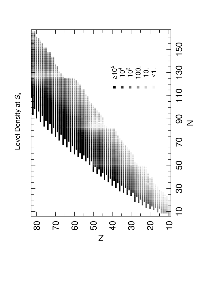
Figure 1.  : Level density (in levels per MeV) at the respective neutron separation energy [Rauscher et al. (1995b), Rauscher et al. (1996)].

Considerable effort has been put into providing the best possible input functions for the statistical model calculations. Entering Eq. C are particle– and photon–transmission coefficients, width fluctuation corrections, masses, and level densities. The level densities were subject to the largest part of the uncertainties in the most recent cross–section calculations [Cowan et al. (1991)]. It is hoped that the accuracy of the theoretical predictions will be further improved by employing advanced level density descriptions (see Sect. 5.3).

It is often colloquially termed that the statistical model is only applicable for intermediate and heavy nuclei. However, the only necessary condition for its application is a large number of resonances at the appropriate bombarding energies, so that the cross section can be described by an average over resonances. This can be valid for light nuclei in specific cases and on the other hand not valid for intermediate mass nuclei near magic numbers. In the case of neutron–induced reactions a criterion for the applicability can directly be derived from the level density. For astrophysical purposes the projectile energies are quite low by nuclear physics standards. Therefore, the relevant energies will lie very close to the neutron separation energy. Thus, one only has to consider the level density at this energy. As a rule–of–thumb it is usually said that there should be at least 10 levels per MeV for reliable statistical model calculations. The level densities at the appropriate neutron separation energies are shown in Fig. 1 (note that therefore the level density is plotted at a different energy for each nucleus). One can easily identify the magic neutron numbers by the drop in level density, as well as odd–even staggering effects. A general sharp drop is also found for nuclei close to the neutron drip line. For nuclei with such low level densities the statistical model cross sections will become very small and other processes might become important, such as direct reactions.

The above plot can give hints on when it is safe to use the statistical model approach and which nuclei have to be treated with special attention at a given temperature. Thus, information which nuclei might be of special interest for an experimental investigation may also be extracted. However, such plots can only give clues as to which reactions have to be studied more carefully as, e.g., the “sufficient number of levels” is only an estimate. Reactions in the temperature range $0\leq T_{9}\leq 0.01$ should always be treated with special care because of the possible importance of single resonances (which can be included in the CN calculation when known; cf., Eq. C).

4.5 Microscopic methods

Microscopic methods like the Resonating Group Method (RGM) or Generator Coordinate method (GCM) start from nucleon–nucleon interactions and are based on many–nucleon wave functions of the nuclei involved. In this approach, the explicit inclusion of the Pauli principle leads to highly nonlocal potentials for the interaction between the composite nuclei in the entrance and exit channel. It is obvious that a fully microscopic approach like RGM and GCM is more satisfying, since it is a first–principle approach.

The main drawback of the RGM is that it requires extensive analytical calculations without systematic character when going from one reaction to another. Consequently, the application of the RGM is essentially restricted to reactions involving only a small number of nucleons. This problem can be overcome by the GCM [Hill and Wheeler (1953)]. In the GCM the relative wave functions are expanded in a Gaussian basis. The GCM is similar to the RGM, but it allows systematic calculations, well suited for a numerical approach.

A microscopic model starts from the nucleon–nucleon interactions and should not contain any free parameter. Therefore, it is possible to predict physical properties of the system independently of experimental data. However, in most cases the fully microscopic approach rarely reproduces physical observables to which the calculations of astrophysical cross sections are sensitive, such as thresholds, resonance and bound–state energies or scattering data. Even if the nucleon–nucleon interaction in microscopic calculations is fitted to reproduce one such relevant observable, other sensitive observables often cannot be reproduced simultaneously. Nevertheless, microscopic methods have also been used extensively for the investigation of astrophysical relevant cross sections and many interesting results have been obtained. Review articles on microscopic theories including examples of astrophysical processes are found in ? (?, ?, ?), ? [Baye and Descouvemont (1988)], ? [Oberhummer and Staudt (1991)], ? [Descouvemont (1993)], and ? [Langanke and Barnes (1996)].

4.6 Direct–reaction models

Direct–reaction (DI) models are based on the description of the dynamics of the reaction by a Schrödinger equation with local optical potentials in the entrance and/or exit channels. Such models are the Distorted Wave Born Approximation (DWBA) [Austern (1970), Satchler (1983), Glendenning (1983), Oberhummer and Staudt (1991)] for transfer or the Direct Capture model (DC) [Christy and Duck (1961), Tombrello and Parker (1963), Rolfs (1973), Oberhummer and Staudt (1991)] for capture reactions. The expressions for the DWBA and DC cross sections are given in Appendix D.

The DI models can be derived from microscopic theories essentially by allowing approximations in the antisymmetrization procedure [Wildermuth and Tang (1977)]. In principle, DI models neglect the antisymmetrization of the optical potentials in the entrance and exit channel as well as exchange processes. However, the effects of the Pauli principle can be taken into account phenomenologically by fitting the parameters of the optical potentials to elastic scattering data or to phase shifts obtained from microscopic models. Furthermore, also exchange processes such as knock out and heavy–particle pickup and stripping have to be considered in some cases. This may be necessary, e.g., to describe differential reaction cross sections on light target nuclei.

The DWBA and DC are based on the premise that elastic scattering in the entrance and exit channel is dominant compared to the flux into other channels. The DWBA and DC are well established for higher projectile energies ($\geq 10-20$ MeV) and transitions to low–lying states of the residual nucleus. For lower energies precompound (e.g., exciton) or compound (e.g., Hauser–Feshbach) models have to be used. However, as stated before, for thermonuclear or thermal energies target nuclei can sometimes have very low level densities. In these cases the contributions from the CN mechanism can be small and the DI mechanism cannot be neglected and may even dominate the reaction.

Important for the success of the DI models is the fact that the optical potentials are taken from realistic models, i.e., from semi–microscopic formalisms such as the folding–potential model, and not only from empirical potentials like Saxon–Woods potentials. Folding potentials have been used extensively and successfully in potential–model calculations for astrophysically relevant nuclear reactions. The folding procedure is used for calculating the real parts of the optical or bound–state potentials to describe the elastic scattering data or the bound states, respectively. In most astrophysical applications one of the particles is a nucleon (proton or neutron), $\alpha$–particle, deuteron, triton or helion. In the folding approach the nuclear density $\rho_{A}$ is folded with an energy and density dependent nucleon–nucleon interaction $v_{\rm eff}$ [Kobos et al. (1984), Oberhummer and Staudt (1991)]. For a nucleon–nucleus system we use single folding

$$V(R)=\lambda\int\;d{\bf r}\rho_{A}({\bf r})v_{\rm eff}(E,\rho_{A},|{\bf R}-{\bf r}|)$$ (8)

and, for a system with both interacting nuclei having mass numbers $A\geq 2$, double folding

$$V(R)=\lambda\int\;d{\bf r_{1}}d{\bf r_{2}}\rho_{A}\left({\bf r_{1}}\right)\rho_{a}\left({\bf r_{2}}\right)v_{\rm eff}\left(E,\rho_{a},\rho_{A},\left|{\bf R}-{\bf r_{1}}-{\bf r_{2}}\right|\right)\quad.$$ (9)

In the above expressions $A$ and $a$ are the two colliding nuclei and ${\bf{R}}$ is the separation of their centers–of–mass. The normalization factor $\lambda$ is adjusted to reproduce the experimental elastic–scattering and separation–energy data for the different channels involved in the considered reaction. This is of special importance for the calculation of astrophysically relevant cross sections, because the correct results of such calculations depend sensitively on the reproduction of the above observables. Also, because at low energies only a few channels are open (sometimes only two or three), only a small or even no imaginary part of the optical potentials, describing absorption into other channels, is necessary.

Section 5 Selected examples

In this section we consider three selected examples: neutron capture on ³⁶S [Beer et al. (1995b), Oberhummer et al. (1995)], ²⁰⁸Pb [Corvi et al. (1995)] and on Gd–isotopes [Wisshak et al. (1995), Rauscher et al. (1995a)].

The main emphasis will be given to the first reaction, because in this case the reaction mechanism is predominantly direct and is therefore sensitive to the details of nuclear structure. Often such reactions have been investigated erroneously using the Hauser–Feshbach method. However, as already stated before, if there are no or only a few CN levels in the energy region of interest, the direct reaction mechanism can even dominate the reaction. There are other recent examples for neutron capture that have been investigated and show a dominance of the direct mechanism: e.g., ¹²C(n,$\gamma$)¹³C [Otsuka et al. (1994), Mengoni et al. (1995)], ¹⁵N(n,$\gamma$)¹⁶N [Meißner et al. (1996)], ¹⁸O(n,$\gamma$)¹⁹O [Grün et al. (1995), Meißner et al. (1995b)], and ⁴⁸Ca(n,$\gamma$)⁴⁹Ca [Krausmann et al. (1996), Beer et al. (1996a)]. Since the reaction ³⁶S(n,$\gamma$)³⁷S involves nuclei at the border of the region of stability, it is also a benchmark for nuclear–structure calculations necessary for nuclei far–off stability.

In the reaction ²⁰⁸Pb(n,$\gamma$)²⁰⁹Pb the DI and CN mechanism give similar values for the cross section in the astrophysical energy range. We compare the resonant and non–resonant contributions of the capture cross section at thermonuclear energies with experimental data. There are other examples for neutron capture by magic target nuclei (e.g., ⁸⁶Kr, ⁸⁸Sr, ¹³⁶Ba, ¹³⁸Ba), where direct capture cannot be neglected [Balogh et al. (1994)].

The usual method to calculate neutron–induced reactions at thermonuclear energies is the statistical Hauser–Feshbach method (cf., Sect. 4.4). However, as stated before, this is only correct if the level density is high enough and the CN mechanism is dominating. This will be the case for the majority of nuclear reactions to be considered in nuclear astrophysics. As one example for a dominating CN mechanism we discuss neutron capture by Gd–isotopes at thermonuclear energies and compare the values for the cross section obtained in the Hauser–Feshbach formalism with the experimental values.

Table III
: Final states, Q–values, transitions and cross sections for ³⁶S(n,$\gamma$)³⁷S at 25.3 meV, 25 keV, 151 keV, 176 keV, and 218 keV using DC with the experimental data.

Final	Q–value	Transition	Cross section
state	[MeV]		25.3 meV	25 keV	151 keV	176 keV	218 keV
			[mbarn]	[$\mu$barn]	[$\mu$barn]	[$\mu$barn]	[$\mu$barn]
$\frac{7}{2}^{-}$	4.303	d $\rightarrow$ f	0.0	0.0	0.1	0.2	0.2
$\frac{3}{2}^{-}$	3.657	s $\rightarrow$ p	157.1	158.0	64.3	59.5	53.5
$\frac{3}{2}^{+}$	2.906	p $\rightarrow$ d	0.0	0.0	0.0	0.0	0.0
$\frac{3}{2}^{-}$	2.312	s $\rightarrow$ p	5.3	5.3	2.1	2.0	1.8
$\frac{1}{2}^{-}$	1.666	s $\rightarrow$ p	28.3	28.5	11.6	10.8	9.7
Total cross section: DC			190.7	191.8	78.1	72.5	65.2
Total cross section: experiment			$150\pm 30$1	$187\pm 14$	$81\pm 7$	$125\pm 11$	$78\pm 7$

¹ ? [Sears (1992)]

5.1 Direct neutron capture by ³⁶S

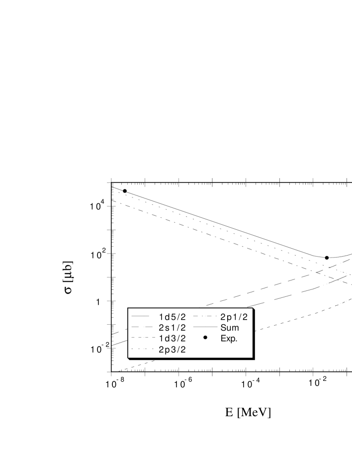
Figure 2.  : Comparison of the DC cross section for ³⁶S(n,$\gamma$)³⁷S with the experimental data from thermal to thermonuclear projectile energies. The DC contributions for the different transitions to the final states of ³⁷S as well as the sum of all transitions (solid curve) are shown. The experimental data at the thermal energy have been taken from ? ?.

For the rare isotope ³⁶S a significant abundance contribution is expected from s–process nucleosynthesis. For quantitative analyses the size of the destruction rate, the neutron capture rate, is of fundamental importance to estimate the magnitude of the ³⁶S abundance formed by the weak and main s–process components. Using the statistical model the ³⁶S capture cross section has been estimated to be 300 $\mu$barn at 30 keV by ? [Woosley et al. (1978)] and 297 $\mu$barn at 30 keV by ? [Cowan et al. (1991)] (1 eV = $1.60219\times 10^{-19}$ J; 1 barn = 10^-24 cm²).

We investigate the capture reaction ³⁶S(n,$\gamma$)³⁷S from thermal (25.3 meV) to thermonuclear (25 –218 keV) projectile energies and compare the calculated cross sections in the DC–model with the experimental data. The experimental investigation was performed using the fast cyclic activation technique [Beer et al. (1994b)] developed at the Karlsruhe 3.75 MV Van de Graaff accelerator.

In the folding approach the nuclear density $\rho_{A}$ for the stable nucleus ³⁶S was derived from the experimental charge distribution [De Vries et al. (1987)]. The normalization factor $\lambda$ of the optical potential in the entrance channel was adjusted to fit the thermal (³⁶S+n)–scattering cross section of ($1.1\pm 0.8$) barn [Sears (1992)]. Although this cross section is not determined well, we fitted our normalization factor to reproduce 1.1 barn. However, applying the same fitting procedure to the (³⁴S+n)–scattering cross section that is known much better (($1.52\pm 0.03$) barn, ?, ?) we obtained almost the same volume integral per nucleon in the two cases (³⁴S+n: 501.7 MeV fm³; ³⁶S+n: 497.1 MeV fm³). The imaginary part of the optical potential is small for the (³⁶S+n)–channel and can be neglected. For the exit channels the normalization constants $\lambda$ were adjusted to the energies of the ground and the excited states. The potentials obtained in this way ensure the correct behavior of the wave functions in the nuclear exterior.

The spectroscopic factors for one–nucleon stripping of ³⁷S were determined from the most recent experimental ³⁶S(d,p)³⁷S–data [Endt (1990)]. The masses and Q–values for the transitions to the different states of the residual nucleus ³⁷S were taken from experimental data [Audi and Wapstra (1993), Endt (1990)]. For the DC–calculations the code TEDCA [Grün and Oberhummer (1995)] was used.

The cross section for the reaction ³⁶S(n,$\gamma$)³⁷S obtained from the DC–calculation is compared to the experimental data from the thermal to the thermonuclear energy region in Fig. 2. There are two types of E1–transitions contributing to the transitions to the residual nucleus ³⁷S. The first one arises from an s–wave in the entrance channel exciting the negative–parity states 3/2^- and 1/2^- (see Table III). These transitions give the well–known 1/v–behavior (see Fig. 2). The second type of E1–transition comes from an initial p–wave and excites the positive–parity state 3/2⁺ in the final nucleus. This transition has a v–behavior and can be neglected in the relevant energy range (see Fig. 2 and Table III). The E1–transition to the 7/2^-–ground state of ³⁷S can be neglected also, because of the higher centrifugal barrier of the incoming d–wave (see Table III). As can be seen from Fig. 2 this contribution affects the deviation from an 1/v–behavior of the cross section only above about 700 keV.

The spin and parity assignments of the final states in ³⁷S and the Q–values for the transitions to the different final states are shown in Table III. Also the calculated cross sections for ³⁶S(n,$\gamma$)³⁷S at 25.3 meV, 25, 151, 176, and 218 keV using DC with the spectroscopic factors obtained from the (d,p)–data are compared with the experimental data in this table. Direct–capture calculations using the folding procedure can excellently reproduce the non–resonant experimental data for the capture cross section by the neutron–rich sulfur isotope ³⁶S in the thermal and thermonuclear energy region. The enhancement in the region of 176 keV comes from resonant contributions [Endt (1990)] not considered in the DC–calculation.

We have determined the thermonuclear reaction rate $N_{A}\left<\sigma v\right>$ [Fowler et al. (1967)]. Since the cross section follows an 1/v–law up to 150 keV we obtain a constant reaction rate (c.f., App. A)

$$N_{A}\left<\sigma v\right>=2.56\times 10^{4}\,{\rm cm}^{3}\,{\rm mole}^{-1}\,{\rm s}^{-1}\quad.$$ (10)

The s–process production of ³⁶S was recently discussed quantitatively by ?, [Schatz et al. (1995)] but without a reliable ³⁶S(n,$\gamma$) cross section. The s–process reaction network in the sulfur to calcium region contains (n,$\gamma$), (n,p), and (n,$\alpha$) reactions. The ³⁶S production is mediated by the ³⁶Cl(n,p)³⁶S reaction from seed nuclei with mass numbers $A<36$. But also seed nuclei $A>36$ can contribute through the ³⁹Ar(n,$\alpha$)³⁶S reaction channel. Besides its formation, the destruction of ³⁶S by the (n,$\gamma$) reaction is important. A decrease in the ³⁶S(n,$\gamma$)³⁷S cross section leads to a corresponding increase of the abundance formed. As our measured ³⁶S(n,$\gamma$)³⁷S value is smaller by a factor of 1.8 than the estimate of Woosley et al. [Woosley et al. (1978)] the s–process abundance production of ³⁶S will be enhanced by this factor. The quantitative analysis requires also model parameters for the main and especially the weak s–process component. This information can be obtained from the analysis of the s–process beyond $A=56$ [Beer et al. (1995a)].

DC could also be the dominant reaction mechanism for neutron capture by neutron–rich isotopes far–off stability occurring in the $\alpha$–rich freeze–out and r–process. Leaving the line of stability, the Q–value and therefore the excitation energy of the compound nucleus becomes lower, leading to a substantial diminuition of the level density of the compound nucleus. Thus, the DC–contribution can become the dominating reaction mechanism. Nuclear–structure models are indispensable for extrapolating reaction rates to nuclei near and far–off the region of stability, because only a limited or no experimental information is available in this region.

The DC cross section of the reaction ³⁶S(n,$\gamma$)³⁷S can be considered as a benchmark for different nuclear–structure models (Shell Model, Relativistic Mean Field Theory, Hartree Fock Bogoliubov Theory) for calculating neutron–capture cross sections by neutron–rich nuclei off–stability taking place in the $\alpha$–rich freeze–out or r–process [Oberhummer et al. (1995)]. We find discrepancies of about a factor of two for the DC cross sections with input parameters from the nuclear–structure models in the case of ³⁶S(n,$\gamma$)³⁷S. For astrophysical applications in nuclear–network calculations such discrepancies can be acceptable sometimes. Clearly, investigations of nuclear–structure models in the manner shown above are necessary to test the reliability of such models for the application to calculations of cross sections of astrophysically relevant nuclear reactions involving nuclei far–off stability.

Table IV
: The resonance and direct capture component of the Maxwellian–averaged cross section $\sigma$ as a function of stellar temperature $k_{\rm B}T$ [Corvi et al. (1995)].

$k_{\rm B}T$	$\sigma$
(keV)	(mbarn)
	resonant	direct	total
	capture	capture	capture
	(exp)	(theory)	(exp+theory)
5	0.0015$\pm$0.0001	0.056$\pm$0.011	0.058$\pm$0.011
8	0.018$\pm$0.001	0.070$\pm$0.014	0.088$\pm$0.014
10	0.039$\pm$0.003	0.079$\pm$0.016	0.118$\pm$0.016
12	0.063$\pm$0.005	0.086$\pm$0.017	0.149$\pm$0.018
15	0.102$\pm$0.009	0.096$\pm$0.019	0.198$\pm$0.021
17	0.126$\pm$0.012	0.102$\pm$0.020	0.228$\pm$0.023
20	0.157$\pm$0.017	0.111$\pm$0.022	0.268$\pm$0.028
25	0.196$\pm$0.023	0.124$\pm$0.025	0.320$\pm$0.034
30	0.221$\pm$0.027	0.135$\pm$0.027	0.356$\pm$0.038
35	0.235$\pm$0.029	0.145$\pm$0.029	0.380$\pm$0.041
40	0.241$\pm$0.029	0.153$\pm$0.031	0.394$\pm$0.042
45	0.243$\pm$0.025	0.162$\pm$0.032	0.405$\pm$0.041
50	0.241$\pm$0.028	0.169$\pm$0.034	0.410$\pm$0.044
60	0.231$\pm$0.026	0.180$\pm$0.036	0.411$\pm$0.044
70	0.216$\pm$0.023	0.189$\pm$0.038	0.405$\pm$0.044
80	0.201$\pm$0.021	0.194$\pm$0.039	0.395$\pm$0.044
90	0.186$\pm$0.015	0.195$\pm$0.039	0.381$\pm$0.042
100	0.171$\pm$0.017	0.195$\pm$0.039	0.366$\pm$0.043

Table V
: Experimental data and Hauser–Feshbach calculations for Maxwellian–averaged cross sections at 30 keV in mbarn for neutron capture on Gd–isotopes.

Target	? [Wisshak et al. (1995)] (exp.)	Hauser–Feshbach (theor.)
152Gd	1049$\pm$17	870
154Gd	1028$\pm$12	622
155Gd	2648$\pm$30	2340
156Gd	615$\pm$5	455
157Gd	1369$\pm$15	1426
158Gd	324$\pm$3	265

5.2 Neutron capture by ²⁰⁸Pb

The s–process of stellar nucleosynthesis terminates at the isotopes of Pb and Bi, since all further neutron capture leads to $\alpha$–unstable nuclei that are then cycled back to the main lead isotopes. To explain the abundances of these isotopes, the so–called strong s–process component was introduced. To study its characteristics in particular the neutron–capture cross section of ²⁰⁸Pb is needed.

Recently, it became possible to determine the resonant part of the capture cross section for ²⁰⁸Pb(n,$\gamma$)²⁰⁹Pb from experiment [Corvi et al. (1995)]. In that work high resolution neutron capture measurements were carried out to determine twelve resonances in the range 1–400 keV (Table I; see also Sec. 3.1). From the data of Table I the resonant Maxwellian–averaged capture (MAC) cross sections (compound capture) were calculated (second column of Table IV), using the Breit–Wigner formalism.

Using the experimentally known density distributions [De Vries et al. (1987)], masses [Audi and Wapstra (1993)] and energy levels [Martin (1991)], we calculated the non–resonant contribution in the DC model. The strength parameter $\lambda$ of the folding potential in the entrance channel was fitted to experimental scattering data at low energies [Sears (1992)]. The value of $\lambda$ for the bound state in the exit channel is fixed by the requirement of correct reproduction of the binding energies. The spectroscopic factors for the relevant low lying states of ²⁰⁹Pb are close to unity as can be inferred from different ²⁰⁸Pb(d,p)²⁰⁹Pb reaction data [Martin (1991)]. The results for the non–resonant MAC (direct capture) cross section can then also be calculated (third column of Table IV).

The total MAC cross section is computed as the sum of the resonant part determined from experiment and the non–resonant part from theory (last column of Table IV). The obtained total MAC cross section at 30 keV of ($0.356\pm 0.038$) mbarn is in excellent agreement with the value obtained from the activation experiment ($0.36\pm 0.03$) mbarn of ? [Ratzel (1988)], thus resolving the previously assumed “contradiction” between the experiments (see also Sec. 3.1).

5.3 Neutron capture on Gd–isotopes

Gadolinium is one of six elements with two even s–only isotopes (¹⁵²Gd and ¹⁵⁴Gd). Such isotopes are important in the detailed investigation of the related s–process branchings which can help to limit the physical conditions in the helium burning zones of Red Giants (cf., Sect. 2.1). Neutron capture on ¹⁴⁷Gd is also of interest in theoretical studies concerning the so–called $\gamma$–process in supernovae of type II, suggested by ? [Woosley and Howard (1978)], and by ? [Rayet et al. (1990)]. In the case of Gd, the level density is high enough so that the direct–capture contribution is negligible and calculations can be restricted to the pure statistical model.

The statistical model (Hauser–Feshbach) is described in more detail in Sect. 4.4. For the statistical model calculations presented in this section, we used the code SMOKER as described in ? [Cowan et al. (1991)], but with an improved level density description based on ? [Ignatyuk et al. (1975)] and ? [Iljinov et al. (1992)], including thermal damping of shell effects. The level densities were the subject to the largest uncertainties in the most recent cross section calculations [Cowan et al. (1991)]. The new description (?, ?, ?, ?) reduces the number of parameters compared to the best global fit as given in ? [Cowan et al. (1991)] while lowering the mean deviation from experimental data considerably (from a factor more than 3 down to a factor of about 1.5) and is expected to give a similar improvement for the accuracy of level densities for nuclei far from stability. Concerning masses, we made use of the most recent mass table [Audi and Wapstra (1993)] and the mass formula by ? [Möller et al. (1995)] where experimental information was not available.

Recently, stellar neutron capture cross sections for the Gd–isotopes with the mass numbers $A$=152, 154, 155, 156, 157, and 158 have been determined experimentally by ? [Wisshak et al. (1995)]. In order to test the approach taken to calculate neutron capture on ¹⁴⁸Gd [Rauscher et al. (1995a)], we compared our results to the experimental cross sections (see Table V). This experimental data has been obtained using the total absorption detection employing a ball of scintillation crystals as described in Sect. 3.1.2.

As can be seen, the values agree reasonably well, especially for odd targets. It has to be emphasized, however, that no parameters of the level density description were adjusted especially to the Gd region, in order to preserve the reliable predictive power for unstable isotopes from a global parameter fit. Further work on improving the statistical model calculations is in progress, and it is estimated that the theoretical cross sections will get a global accuracy of about 30% in future calculations.

Appendix

Section A Astrophysical reaction rates

The quantity most often quoted when dealing with nuclear reactions in astrophysics is the nuclear reaction rate, measuring the number of reactions per particle pair per second (it can also be generalized to reactions involving more than two nuclei). It can be calculated from the nuclear cross section $\sigma$ for a given reaction by folding it with the velocity (i.e., energy) distribution of the particles involved. In most astrophysical applications the nuclei are in a thermalized plasma, yielding a Maxwell-Boltzmann velocity distribution. The astrophysical reaction rate $R$ at a temperature $T$ can then be written as [Fowler et al. (1975)]

$$R(T)=\left<\sigma v\right>=\left(\frac{8}{\pi m}\right)^{1/2}\frac{1}{(k_{\rm B}T)^{3/2}}\int_{0}^{\infty}\sigma(E)E\exp\left(-\frac{E}{k_{\rm B}T}\right)\,dE\quad,$$ (11)

with the reduced mass $m$ of the interacting particles and the Boltzmann constant $k_{\rm B}$.

The threshold behavior of reaction cross sections is fundamental in nuclear astrophysics because of the small projectile energies in the thermonuclear region. Near the threshold the reaction cross section can be written [Blatt and Weisskopf (1962)]

$$\sigma_{if}=\frac{\pi}{k^{2}}\frac{-4kR{\rm Im}f_{0}}{\left|f_{0}\right|^{2}}\quad,$$ (12)

where $f_{\ell}$ is the logarithmic derivative of the scattering wave function for the $\ell$–th partial wave at an appropriate nuclear radius $R$

$$f_{\ell}=R\left(\frac{1}{u_{\ell}(r)}\frac{du_{\ell}(r)}{dr}\right)_{r=R}=R\left(\frac{d\ln u_{\ell}(r)}{dr}\right)_{r=R}\quad.$$ (13)

Since the logarithmic derivative $f_{0}$ of the scattering wave function is only weakly dependent on the projectile energy, one obtains for low energies the well–known 1/v–behavior.

With increasing neutron energy higher partial waves with $\ell>0$ contribute more significantly to the reaction cross section. Thus the product $\sigma v$ becomes a slowly varying function of the neutron velocity and one can expand this quantity into an expansion in terms of $v$ or $\sqrt{E}$ around zero energy:

$$\sigma v=S(0)+\dot{S}(0)\sqrt{E}+\ddot{S}(0)E+\ldots\quad.$$ (14)

The quantity $S(E)=\sigma v$ is the astrophysical S–factor for neutron–induced reactions and the dotted quantities represent derivatives with respect to $E^{1/2}$. Notice that the above astrophysical S–factor for neutron–induced reactions is different from that for charged–particle induced reactions. In the astrophysical S–factor for charged–particle induced reactions also the penetration factor through the Coulomb barrier has to be considered.

Inserting this into Eq. 11 we obtain for the reaction rate for neutron–induced reactions

$$\left<\sigma v\right>=S(0)+\left(\frac{4}{\pi}\right)^{\frac{1}{2}}\dot{S}(0)(k_{\rm B}T)^{\frac{1}{2}}+\frac{3}{4}\ddot{S}(0)k_{\rm B}T+\ldots\quad.$$ (15)

In most astrophysical neutron–induced reactions, neutron s–waves will dominate, resulting in a cross section showing a 1/$v$–behavior (i.e., $\sigma(E)\propto 1/\sqrt{E}$). In this case, the reaction rate will become independent of temperature, $R={\rm const}$. Therefore it will suffice to measure the cross section at one temperature in order to calculate the rates for a wider range of temperatures. Experiments using neutrons with a Maxwell-Boltzmann energy distribution (of a temperature $T$) directly measure the so–called Maxwellian Averaged Capture (MAC) Cross Sections $\left<\sigma\right>_{T}$. The rate can then be computed very easily by using

$$R=\left<\sigma v\right>=\left<\sigma\right>_{T}v_{T}={\rm const}\quad,$$ (16)

with

$$v_{T}=\left(\frac{2kT}{m}\right)^{1/2}\quad.$$ (17)

The mean lifetime $\tau_{\rm n}$ of a nucleus against neutron capture, i.e., the mean time between subsequent neutron captures is inversely proportional to the available number of neutrons $N_{\rm n}$ and the reaction rate $R_{\rm n\gamma}$:

$$\tau_{\rm n}=\frac{1}{N_{\rm n}R_{\rm n\gamma}}\quad.$$ (18)

If this time is shorter than the beta–decay half–life of the nucleus, it will be likely to capture a neutron before decaying. In this manner, more and more neutrons can be captured to build up nuclei along an isotopic chain until the beta–decay half–life of an isotope finally becomes shorter than $\tau_{\rm n}$. With the very high neutron densities encountered in several astrophysical scenarios, isotopes very far–off stability can be synthesized.

Section B Expressions for cyclic activation

The time constants for each cycle adjusted to the decay rate $\lambda$ of the investigated isotope are the irradiation time $t_{\rm b}$, the counting time $t_{\rm c}$, the waiting time $t_{\rm w}$ (the time to switch from the irradiation to the counting phase), and the total time $T=t_{\rm b}+t_{\rm w}+t_{\rm c}+t^{\prime}_{\rm w}$ ($t^{\prime}_{\rm w}$ the time to switch from the counting to the irradiation phase). The accumulated number of counts from a total of $n$ cycles, $C=\sum_{i=1}^{n}C_{i}$, with the $C_{i}$, the counts after the i–th cycle, irradiated by a neutron flux $\Phi_{i}$, given by

$$C = \epsilon_{\gamma}K_{\gamma}f_{\gamma}[1-\exp(-\lambda t_{\rm c})]\frac{\exp(-\lambda t_{\rm w})}{1-\exp(-\lambda T)}N\sigma[1-f^{\prime}_{\rm b}\exp(-\lambda T)]$$

$$\times\sum_{i=1}^{n}\int_{0}^{t_{\rm b}}\Phi_{i}\exp(-\lambda t)dt\quad,$$

with

$$f^{\prime}_{\rm b}=\frac{\sum_{i=1}^{n}\int_{0}^{t_{b}}\Phi_{i}\exp(-\lambda t)\exp[-(n-i)\lambda T]dt}{\sum_{i=1}^{n}\int_{0}^{t_{b}}\Phi_{i}\exp(-\lambda t)dt}\quad.$$

The activities of nuclides with half–lives of several hours to days can also be counted after the end of the cyclic activation consisting of $n$ cycles:

$$C_{n} = \epsilon_{\gamma}K_{\gamma}f_{\gamma}[1-\exp(-\lambda T_{\rm M})]\exp(-\lambda T_{\rm W})N\sigma f^{\prime}_{b}$$

$$\times\sum_{i=1}^{n}\int_{0}^{t_{\rm b}}\Phi_{i}\exp(-\lambda t)dt\quad.$$

Here $T_{\rm M}$ is the measuring time of the Ge–detector and $T_{\rm W}$ the time elapsed between the end of cyclic activation and beginning of the new data acquisition.

In the application of the cyclic activation method the irradiation time $t_{\rm b}$ is chosen to be short compared to the fluctuations of the neutron flux so that one can integrate [Beer et al. (1994b)]:

$$\int_{0}^{t_{\rm b}}\Phi_{i}\exp(-\lambda t)dt=\lambda^{-1}[1-\exp(-\lambda t_{\rm b})]\Phi_{i}\quad.$$

Section C Hauser–Feshbach formula

The Hauser–Feshbach formula is given by

$$\sigma^{\mu\nu}_{i}(j,o;E) = \frac{\pi\hbar^{2}}{(2\mu_{\alpha}E)(2J^{\mu}_{i}+1)(2J_{j}+1)}$$

$$\times\sum_{J,\pi}(2J+1)\frac{T^{\mu}_{j}(E,J,\pi,E^{\mu}_{i},J^{\mu}_{i},\pi^{\mu}_{i})T^{\nu}_{o}(E,J,\pi,E^{\nu}_{m},J^{\nu}_{m},\pi^{\nu}_{m})}{T_{\rm tot}(E,J,\pi)}$$

for the reaction $i^{\mu}(j,o)m^{\nu}$ from the target state $i^{\mu}$ to the exited state $m^{\nu}$ of the final nucleus, with center of mass energy $E$ and reduced mass $\mu$. The angular momentum quantum number $J$ denotes the spin, $E$ the excitation energy, and $\pi$ the parity of excited states. When these properties are used without subscripts they describe the compound nucleus, subscripts refer to states of the participating nuclei in the reaction $i^{\mu}(j,o)m^{\nu}$ and superscripts indicate the specific excited states. Experiments measure $\sum_{\nu}\sigma_{i}^{0\nu}(j,o;E)$, summed over all excited states of the final nucleus, with the target in the ground state. Target states $\mu$ in an astrophysical plasma are thermally populated and the astrophysical cross section $\sigma^{*}_{i}(j,o)$ is given by

$$\sigma^{*}_{i}(j,o;E)=\frac{\sum_{\mu}(2J^{\mu}_{i}+1)\exp\left(-\frac{E^{\mu}_{i}}{k_{\rm B}T}\right)\sum_{\nu}\sigma^{\mu\nu}_{i}(j,o;E)}{\sum_{\mu}(2J^{\mu}_{i}+1)\exp\left(-\frac{E^{\mu}_{i}}{k_{\rm B}T}\right)}\quad.$$ (22)

The summation over $\nu$ replaces $T_{o}^{\nu}(E,J,\pi)$ in Eq. C by the total transmission coefficient

$$T_{o}(E,J,\pi) = \sum^{\nu_{m}}_{\nu=0}T^{\nu}_{o}(E,J,\pi,E^{\nu}_{m},J^{\nu}_{m},\pi^{\nu}_{m})$$

$$+\int\limits_{E^{\nu_{m}}_{m}}^{E-S_{m,o}}\sum_{J_{m},\pi_{m}}T_{o}\left(E,J,\pi,E_{m},J_{m},\pi_{m}\right)\rho\left(E_{m},J_{m},\pi_{m}\right)dE_{m}\quad.$$

Here $S_{m,o}$ is the channel separation energy, and the summation over excited states above the highest experimentally known state $\nu_{m}$ is changed to an integration over the level density $\rho$. The summation over target states $\mu$ in Eq. 22 has to be generalized accordingly.

Section D Expressions for DC and DWBA

The differential cross section for the transfer reaction $a+A\rightarrow b+B$ with $a-x=b$, $A+x=B$ (stripping) using light projectiles and ejectiles (for $a\leq 4$ and $x=1$ or $x=3$) is given in zero–range DWBA by [Satchler (1983), Glendenning (1983)]

$$\frac{d\sigma}{d\Omega}=\frac{\mu_{\alpha}\mu_{\beta}}{(2\pi\hbar^{2})^{2}}\frac{k_{\beta}}{k_{\alpha}}\frac{2I_{B}+1}{2I_{A}+1}\sum_{\ell sj}C^{2}{\cal S}_{\ell j}N\frac{\sigma_{\ell sj}(\vartheta)}{2s+1}$$ (24)

with the zero–range normalization constant

$$N=\frac{1}{2}aD_{0}^{2}\quad.$$ (25)

The reduced cross section without spin–orbit coupling is

$$\sigma_{\ell sj}(\vartheta)=\sum_{m}\left|t_{\ell sj}^{m}\right|^{2}$$ (26)

with the reduced transition amplitude

$$t_{lsj}^{m}=\frac{1}{2\ell+1}\int\;d{\bf r}\chi_{\beta}^{(-)*}\left({\bf k}_{\beta},{A}{B}{\bf r}\right)u_{\ell j}(r)[i^{\ell}Y_{\ell}^{m}({\bf\hat{r}})]^{*}\chi_{\alpha}^{(+)}({\bf k}_{\alpha},{\bf r})\quad.$$ (27)

The quantities $\mu_{\alpha}$, $\mu_{\beta}$ and $k_{\alpha}$, $k_{\beta}$ are the reduced masses and wave numbers in the entrance channel $\alpha$ and exit channel $\beta$, respectively. The spin and magnetic spin quantum numbers of the projectile, ejectile, target and residual nucleus are given by ($I_{\rm a}$, $I_{\rm b}$, $I_{\rm A}$, $I_{\rm B}$) and ($M_{\rm a}$, $M_{\rm b}$, $M_{\rm A}$, $M_{\rm B}$), respectively. The orbital angular momentum quantum number $\ell$, the spin quantum number $s$ and the total angular momentum quantum number $j$ refer to the cluster $x$ bound in the residual nucleus $B$. The optical wave functions in the entrance and exit channels are characterized by $\chi^{(+)}$ and the time–reversed solution $\chi^{(-)}$. The spectroscopic factor and the isospin Clebsch–Gordan coefficient for the partition $B=A+x$ are given by $C$ and ${\cal S}_{\ell j}$, respectively. Expressions similar to the above equations will be obtained if the finite range of the interaction potential is taken into account [Satchler (1983)].

The above expressions are written for a stripping reaction, where the nucleon cluster $x$ is stripped from the projectile $a$. The corresponding formulae for a pick–up reaction can be obtained easily with the help of the reciprocity theorem for the reduced cross sections [Satchler (1983)].

The direct capture process $a+A\rightarrow\gamma+B$, which is entirely electromagnetic, is treated in first–order perturbation theory. As examples, we quote the expressions for the electric dipole E1 capture [Christy and Duck (1961), Rolfs (1973)]:

$$\sigma_{\rm E1} = \frac{16\pi}{9}\left(\frac{E_{\gamma}}{\hbar c}\right)^{3}\frac{e^{2}\mu_{\alpha}^{3}}{\hbar^{2}k_{\alpha}}\frac{3}{\left(2I_{\rm a}+1\right)\left(2I_{\rm A}+1\right)}\left(\frac{Z_{\rm a}}{m_{\rm a}}-\frac{Z_{\rm A}}{m_{\rm A}}\right)^{2}C^{2}{\cal S}_{\ell_{\beta}J_{\beta}}$$ (31)

$$\times\sum_{\ell_{\alpha}J_{\alpha}}\left(2J_{\beta}+1\right)\left(2J_{\alpha}+1\right)\max\left(\ell_{\alpha},\ell_{\beta}\right)$$

$$\times\left\{\begin{array}[]{ccc}1&\ell_{\beta}&\ell_{\alpha}\\ I&J_{\alpha}&J_{\beta}\end{array}\right\}^{2}a_{I}^{2}\left|R_{1\beta\alpha}\right|^{2}$$

with the radial integral

$$R_{1\beta\alpha}=\frac{1}{k_{\alpha}}\int\;dru_{\beta}^{*}(r){\cal O}_{E1}(r)\chi_{\alpha}(r)\quad.$$ (32)

The coefficients $a_{I}^{2}$ are calculated in LS coupling to

$$a_{I}^{2} = (2I+1)\left(2I_{\rm A}+1\right)\left(2L_{\rm B}+1\right)\left(2S_{\rm B}+1\right)$$ (38)

$$\times\left\{\begin{array}[]{ccc}I&L_{\rm A}&S_{\rm B}\cr L_{\rm B}&I_{\rm B}&\ell_{\beta}\end{array}\right\}^{2}\left\{\begin{array}[]{ccc}I&L_{A}&S_{B}\\ I_{\rm A}&I_{\rm a}&I_{\rm A}\end{array}\right\}^{2}\quad.$$

In the above expressions, the energy of the emitted photon is $E_{\gamma}$. The charge and mass of the projectile and target nucleus are $Z_{\rm a}$, $m_{\rm a}$, $Z_{\rm A}$ and $m_{\rm A}$, respectively. The orbital and total angular momentum quantum numbers of the nuclei in the entrance and exit channels are $\ell_{\alpha}$, $J_{\alpha}$, $\ell_{\beta}$ and $J_{\beta}$, respectively. The spin quantum number, the orbital and total angular momentum quantum numbers are characterized by $S$, $L$ and $I$, respectively, with indices $a$, $A$ and $B$ corresponding to the projectile, target and residual nucleus, respectively. The symbol $\left\{\matrix{\ldots}\right\}$ is the $6j$ symbol. The radial wave functions in the entrance and exit channels are given by $\chi_{\alpha}$ and $u_{\beta}$, respectively. The spectroscopic factor and the isospin Clebsch–Gordan coefficient for the partition $B=A+a$ are given by $C$ and ${\cal S}_{\ell_{\beta}J_{\beta}}$, respectively. The ${\cal O}_{{\rm E}\ell}$ are the multipole operators.

References

- Anders and Grevesse (1989) Anders, E. and Grevesse, N.: 1989, Geochim. et Cosmochim. Acta 53, 197.
- Applegate and Hogan (1985) Applegate, J.H. and Hogan, C.J.: 1985, Phys. Rev. D 31, 3037.
- Applegate et al. (1988) Applegate, J.H., Hogan, C.J., and Scherrer, R.J.: 1988, Ap. J. 329, 572.
- Arnett et al. (1971) Arnett, W.D., Truran, J.W., and Woosley, S.E.: 1971, Ap. J. 165, 87.
- Arnould (1972) Arnould, M.: 1972, Astron. and Astrophys. 19, 92.
- Arnould and Rayet (1990) Arnould, M. and Rayet, M.: 1990, Ann. Phys. Fr. 15, 183
- Arnould and Takahashi (1993) Arnould, M. and Takahashi, K.: 1993, in N. Prantzos, E. Vangioni-Flam, and M. Cassé (eds.), Origin and Evolution of the Elements, Cambridge University Press, Cambridge, p. 395.
- Audi and Wapstra (1993) Audi, G. and Wapstra, A.H.: 1993, Nucl. Phys., A565, 1.
- Austern (1970) Austern, N.: 1970, Direct Nuclear Reaction Theories, John Wiley & Sons, New York.
- Balogh et al. (1994) Balogh, W., Bieber, R., Oberhummer, H., Rauscher, T., Kratz, K.-L., Mohr, P., Staudt, G., and Sharma, M.M.: 1994, in E. Somoraj and Z. Fülöp (eds.), Proceedings of the European Workshop on Heavy Element Nucleosynthesis, Budapest, Hungary, Institute of Nuclear Research of the Hung. Acad. of Sci., Debrecen, Hungary, p. 74.
- Baye and Descouvemont (1988) Baye, D. and Descouvemont P.: 1988, in Proc. 5th Int. Conf. on Clustering Aspects in Nuclear and Subnuclear Systems, Kyoto, Japan 1988, J. Phys. Soc. Jpn., Suppl. 58, p. 103.
- Beer and Käppeler (1980) Beer, H. and Käppeler, F.: 1980, Phys. Rev. C 21, 534.
- Beer (1991) Beer, H.: 1991, Ap. J. 375, 823.
- Beer et al. (1991) Beer, H., Rupp, G., Voß, F., and Käppeler, F.: 1991, Ap. J. 379, 420.
- Beer et al. (1992) Beer, H., Wiescher, M., Käppeler, F., Görres, J., and Koehler, P.E.: 1992, Ap. J. 387, 258.
- Beer et al. (1994a) Beer, H., Corvi, F., and Athanassopulos, K.: 1994a, in J. Kern (ed.) Proc. of the 8th Int. Symp. on Capture Gamma–Ray Spectr. and Related Topics, Fribourg, Switzerland, World Scientific, Singapore, p. 698.
- Beer et al. (1994b) Beer, H., Rupp, G., Walter, G., Voß, F., and Käppeler, F.: 1994b, Nucl. Instr. Methods A 337, 492.
- Beer et al. (1995a) Beer H., Spettel, B., and Palme, H.: 1995a, in M. Busso, R. Gallino, and C.M. Raiteri (eds.), Nuclei in the Cosmos, AIP Conf. Proc. 327, 307.
- Beer et al. (1995b) Beer, H., Sedyshev, P.V., Popov, Yu.P., Balogh, W., Herndl, H., and Oberhummer, H.: 1995b, Phys. Rev. C 52, 3442.
- Beer et al. (1996a) Beer, H., Coceva, C., Sedyshev, P.V., Popov, Yu.P., Herndl, H., Hofinger R., Mohr P., and Oberhummer, H.: 1996a, Phys. Rev. C, in press.
- Beer et al. (1996b) Beer, H., Corvi, F., and Oberhummer, H.: 1996b, in E. I. Kornilov (ed.) VII School on Neutron Physics, 3–22 September 1995, Ratmino, Russia, in press.
- Beer et al. (1996c) Beer, H., Corvi, F., and Mutti, P.: 1996c, Ap. J., in press.
- Blatt and Weisskopf (1962) Blatt, J.M. and Weisskopf, V.F.: 1962, Theoretical Nuclear Physics, Wiley & Sons, New York.
- Boesgard and Steigman (1985) Boesgard, A. and Steigman, G.: 1985, Ann. Rev. Astron. Astrophys. 23, 319.
- Bohr (1936) Bohr, N.: 1936, Nature 137, 344.
- Bouquelle et al. (1996) Bouquelle, V., Cerf, N., Arnould, M., Tachibana, T., and Goriely, S.: 1996, Astron. Astrophys. 305, 1005.
- Breit and Wigner (1936) Breit, R.G. and Wigner, E.P.: 1936, Phys. Rev. 49, 519.
- Burbidge et al. (1957) Burbidge, E.M., Burbidge, G.R., Fowler, W.A., and Hoyle, F.: 1957, Rev. Mod. Phys. 29, 547.
- Burrows and Fryxell (1992) Burrows, A. and Fryxell, B.: 1992, Science 258, 430.
- Burrows et al. (1995) Burrows, A., Hayes, J., and Fryxell, B.: 1995, Ap. J. 450, 830.
- Butler (1950) Butler, S.T.: 1950, Phys. Rev. 80, 559.
- Butler (1951) Butler, S.T.: 1951, Proc. Roy. Soc. A 208, 36.
- Cameron (1955) Cameron, A.G.W.: 1955, Ap. J. 121, 144.
- Chen et al. (1995) Chen, J., Dobaczewski, J., Kratz, K.-L., Langanke, K., Pfeiffer, B., Thielemann, F.-K., and Vogel, P.: 1995, Phys. Lett. B 355, 37.
- Christy and Duck (1961) Christy, R.F. and Duck, I.: 1961, Nucl. Phys. 24, 89.
- Coceva (1994) Coceva, C.: 1994, Nuovo Cim. 107, 85.
- Corvi et al. (1991) Corvi, F., Fioni, G., Gasperini, F., and Smith, P.B.: 1991, Nucl. Science Eng. 107, 272.
- Corvi (1995) Corvi, F.: 1995, in C. Coceva, A. Mengoni, and A. Ventura (eds.), Specialists’ Meeting on Measurement, Calculation and Evaluation of Photon Production Data, NEA/NSC/DOC(95)1, p. 229.
- Corvi et al. (1995) Corvi, F., Mutti, P., Athanassopulos, K., and Beer, H.: 1995, in M. Busso, R. Gallino, and C.M. Raiteri (eds.), Nuclei in the Cosmos, AIP Conf. Proc. 327, 165.
- Cowan et al. (1991) Cowan, J.J., Thielemann, F.-K., and Truran, J.W.: 1991, Phys. Rep. 208, 267.
- Descouvemont (1993) Descouvemont P.: 1993, in F. Käppeler and K. Wisshak (eds.), Nuclei in the Cosmos, IOP Publishing Ltd., London, p. 77.
- De Vries et al. (1987) De Vries, H., De Jager, C.W., and De Vries, C.: 1992, At. Data and Nucl. Tables 36, 495.
- Endt (1990) Endt, P.M.: 1990, Nucl. Phys. A 521, 1.
- Fowler et al. (1967) Fowler, W.A., Caughlan, G.R. and Zimmermann, B.A.: 1967, Ann. Rev. Astron. and Astrophys. 5, 525.
- Fowler et al. (1975) Fowler, W.A., Caughlan, G.R. and Zimmermann, B.A.: 1975, Ann. Rev. Astron. and Astrophys. 13, 69.
- Freiburghaus (1995) Freiburghaus, C.: 1995, diploma thesis, University of Basel, Switzerland.
- Gadioli and Hodgson (1992) Gadioli, E. and Hodgson, P.E.: 1992, Pre–Equilibrium Nuclear Reactions, Clarendon Press, Oxford.
- Gallino et al. (1996) Gallino, R., Busso, M., Arlandini, C., Lugaro, M., and Straniero, O.: 1996, Mem. Soc. Astr. It., in press.
- Glendenning (1983) Glendenning, N.K.: 1983, Direct Nuclear Reactions, Academic Press, New York.
- Grün et al. (1995) Grün, K., Pichler, R., and Oberhummer, H.: 1995, in G. Vourvopolous and T. Paradellis (eds.) Neutrons and Their Applications, Proc. SPIE 2339, 77.
- Hauser and Feshbach (1952) Hauser, W. and Feshbach, H.: 1952, Phys. Rev. 87, 366.
- Herant et al. (1992) Herant, M., Benz, W., and Colgate, S.: 1992, Ap. J. 395, 642.
- Herant et al. (1994) Herant, M., Benz, W., Hix, W.R., Fryer, C.L., and Colgate, S.: 1994, Ap. J. 435, 339.
- Hill and Wheeler (1953) Hill, D.L. and Wheeler, J.A.: 1953, Phys. Rev. 89, 1102.
- Holmes et al. (1976) Holmes, J.A., Woosley, S.E., Fowler, W.A., and Zimmerman, B.A.: 1976, At. Data Nucl. Data Tables 18, 306.
- Howard et al. (1993) Howard, W.M., Goriely, S., Rayet, M., and Arnould, M.: 1993, Ap. J. 467, 713.
- Igashira et al. (1994) Igashira, M., Tanaka, K., and Masuda, K.: 1994, in J. Kern (ed.), Proc. 8th Int. Symp. Capture Gamma–Ray Spectroscopy, IOP Publishing Ltd., London, p. 992.
- Ignatyuk et al. (1975) Ignatyuk, A.V., Smirenkin, G.N., and Tishin, A.S.: 1975, Yad. Phys. 21, 485.
- Iljinov et al. (1992) Iljinov, A.S., Mebel, M.V., Bianchi, N., De Sanctis, E., Guaraldo, C., Lucherini, V., Muccifora, V., Polli, E., Reolon, A.R., and Rossi, P.: 1992, Nucl. Phys. A 543, 517.
- Jaag and Käppeler (1995a) Jaag, S., and Käppeler, F.: 1995a, Phys. Rev. C 51, 3465.
- Jaag and Käppeler (1995b) Jaag, S. and Käppeler, F.: 1995b, Phys. Rev. C, submitted.
- Janka and Müller (1993) Janka, H.-T. and Müller, E.: 1993, in Y. Suzuki, and K. Nakamura (eds.), Frontiers of Neutrino Astrophysics, Universal Academy Press, Tokyo, p. 203.
- Janka and Müller (1994) Janka, H.-T. and Müller, E.: 1994, Astron. Astrophys. 290, 496.
- Janka and Müller (1995) Janka, H.-T. and Müller, E.: 1995, Ap. J. Lett. 448, L109.
- Janka and Müller (1996) Janka, H.-T. and Müller, E.: 1996, Astron. Astrophys. 306, 167.
- Kalckar and Bohr (1937) Kalckar, F. and Bohr, N.: 1937, K. Danske Vidensk. Selsk. Mat.-fys. Medd. 14, 10.
- Käppeler et al. (1989) Käppeler, F., Beer, H., and Wisshak, K.: 1989, Rep. Prog. Phys. 52, 945.
- Käppeler et al. (1990a) Käppeler, F., Gallino, R., Busso, M., Picchio, G., and Raiteri, C.M.: 1990a, Ap. J. 354, 630.
- Käppeler et al. (1994) Käppeler, F., Wiescher, M., Giesen, U., Görres, J., Baraffe, I., El Eid, M., Raiteri, C.M., Busso, M., Gallino, R., Limongi, M., Chieffi, A.: 1994, Ap. J. beer437, 396.
- Käppeler et al. (1990b) Käppeler, F., Zhao, W.R., Beer, H., and Ratzel, U.: 1990b, Ap. J. 355, 348.
- Kobos et al. (1984) Kobos, A.M., Brown, B.A., Lindsay, R., and Satchler, G.R.: 1984, Nucl. Phys. A 425, 205.
- Kratz et al. (1988) Kratz, K.-L., Thielemann, F.-K., Hillebrandt, W., Möller, P., Harms, V., Wöhr, A., and Truran J.W.: 1988, J. Phys. G 14, 331.
- Kratz et al. (1993) Kratz, K.-L., Bitouzet, J.-P., Thielemann, F.-K., Möller, P., and Pfeiffer, B.: 1993, Ap. J. 402, 216.
- Kratz et al. (1994) Kratz, K.-L., Möller, P., Pfeiffer, B., and Thielemann, F.-K.: 1994, in J. Kern (ed.), Proc. 8th Int. Symp. Capture Gamma–Ray Spectroscopy, IOP Publishing Ltd., Bristol, p. 724.
- Krausmann et al. (1996) Krausmann, E., Balogh, W., Oberhummer, H., Rauscher, T., Ziegert, W., and Kratz K.-L.: 1995, Phys. Rev. C, 53, 469.
- Grün and Oberhummer (1995) Grün K. and Oberhummer H.: 1995, code TEDCA, TU Wien, unpublished.
- Lane and Thomas (1958) Lane, A.M. and Thomas, R.G.: 1958, Rev. Mod. Phys. 30, 257.
- Langanke (1986) Langanke K.: 1986, in J.W. Negele and E. Vogt (eds.) Nuclear Astrophysics, Plenum Press, New York, p. 223.
- Langanke (1988) Langanke, K., and Friedrich, H.: 1988, in M. Lozano, M.I. Gallardo, and J.M. Arias (eds.), Adv. in Nucl. Phys., 17, 241.
- Langanke (1991) Langanke, K.: 1991, in H. Oberhummer (ed.), Nuclei in the Cosmos, Springer–Verlag, Berlin, New York, p. 61.having
- Langanke and Barnes (1996) Langanke, K. and Barnes C.A.: 1996, in J.W. Negele and E. Vogt (eds.), Adv. in Nucl. Phys., 22, 173.
- Macklin and Gibbons (1967) Macklin, R.L., and Gibbons, J.H.: 1967, Phys. Rev. 159, 1007.
- Macklin et al. (1977) Macklin, R.L., Halperin, J., and Winters, R.R.: 1977, Ap. J. 217, 222.
- Mahaux and Weidenmüller (1979) Mahaux, C. and Weidenmüller, H.A.: 1979, Ann. Rev. Nucl. Part. Sci. 29, 1.
- Malaney and Mathews (1993) Malaney, R.A. and Mathews, G.J.: 1993, Phys. Rep. 229, 145.
- Martin (1991) Martin, M.J.: 1991, Nucl. Data Sheets 63, 723.
- Meißner et al. (1995a) Meißner, J., Schatz, H., Herndl, H., Wiescher, M., Beer, H., and Käppeler, F.: 1995a, in M. Busso, R. Gallino, and C.M. Raiteri (eds.), Nuclei in the Cosmos, AIP Conf. Proc. 327, 307.
- Meißner et al. (1995b) Meißner, J., Schatz, H., Görres J., Herndl, H., Wiescher, M., Beer, H., and Käppeler, F.: 1995b, Phys. Rev. C 53, 459.
- Meißner et al. (1996) Meißner, J., Schatz, H., Herndl, H., Wiescher, M., Beer, H., and Käppeler, F.: 1996, Phys. Rev. C 53, 977.
- Mengoni et al. (1995) Mengoni, A., Otsuka, T., and Ishara, M.: 1995, Phys. Rev. C 52, R2334.
- Meyer (1994) Meyer, B.S.: 1994, Ann. Rev. Astron. Astrophys. 32, 153.
- Michaud and Fowler (1970) Michaud, G. and Fowler, W.A.: 1970, Phys. Rev. C 2, 2041.
- Möller et al. (1995) Möller, P., Nix, J.R., Myers, W.D., and Swiatecki, W.J.: 1995, At. Data Nucl. Data Tables 59, 185.
- Musgrove et al. (1979) Musgrove, A.R. de, Allen, B.J., and Macklin, R.L.: 1979, Aust. J. Phys. 32, 213.
- Nagai et al. (1991a) Nagai, Y., Igashira, M., Mukai, N., Ohsaki, T., Uesawa, F., Takeda, K., Ando, T., Kitazawa, H., Kubono, S., and Fukuda, T.: 1991a, Ap. J. 381, 444.
- Nagai et al. (1991b) Nagai, Y., Igashira, M., Takeda, K., Mukai, N., Motoyama, S., Uesawa, F., Kitazawa, H., and Fukuda, T.: 1991b, Ap. J. 372, 683.
- Nagai et al. (1995) Nagai, Y., Igashira, M., Shima, T., Masuda, K., Ohsaki, T., and Kitazawa, H.: 1995, in M. Busso, R. Gallino, and C.M. Raiteri (eds.), Nuclei in the Cosmos, AIP Conf. Proc. 327, 201.
- Oberhummer and Staudt (1991) Oberhummer, H. and Staudt G.: 1991, in H. Oberhummer (ed.), Nuclei in the Cosmos, Springer–Verlag, Berlin, New York, p. 29.
- Oberhummer et al. (1995) Oberhummer, H., Balogh, W., Bieber, R., Herndl, H., Langer, U., Rauscher, T., and Beer, H.: 1995, Proceedings of the International Conference on Exotic Nuclei and Atomic Masses 1995 (ENAM95), Arles, France, Les Editions Frontières, Gif–sur–Yvette, p. 649.
- Olive et al. (1990) Olive, K., Schramm, D.N., Steigman, G., and Walker, T.: 1990, Phys. Lett. B 236, 454.
- Otsuka et al. (1994) Otsuka, T., Ishara, M., Fukunishi, N., Nakamura, T., and Yokohama, M.: 1994, Phys. Rev. C 49, R2289.
- Palme and Beer (1993) Palme, H. and Beer, H.: 1993, Abundances of the Elements in the Solar System, in H. H. Voigt (ed.), Landolt Börnstein, New Series, Group VI, Astronomy and Astrophysics, Subvolume 3a, Springer Verlag Heidelberg, p. 196
- Perey et al. (1988) Perey, F.G., Johnson, J.O., Gabriel, T.A., Macklin, R.L., Winters, R.R., Todd, J.H., and Hill, N.W.: 1988, in S. Igarasi (ed.), Proc. Int. Conf. on Nucl. Data for Science and Technology, Mito, Japan, Japan Atomic Energy Research Institute, Saikon Pub. Co., Tokyo, p. 379.
- Ratynski and Käppeler (1988) Ratynski, W. and Käppeler, F.: 1988, Phys. Rev. C 37, 595.
- Ratzel (1988) Ratzel U.: 1988, report, KfK Karlsruhe, unpublished.
- Rauscher et al. (1994) Rauscher, T., Applegate, J.H., Cowan, J.J., Thielemann, F.-K., and Wiescher, M.: 1994, Ap. J. 429, 499.
- Rauscher et al. (1995a) Rauscher, T., Thielemann, F.-K., and Oberhummer, H.: 1995a, Ap. J., 451, L37.
- Rauscher et al. (1995b) Rauscher, T., Thielemann, F.-K., and Kratz, K.-L.: 1995b, Mem. Soc. Astr. It., in press.
- Rauscher et al. (1996) Rauscher, T., Thielemann, F.-K., and Kratz, K.-L.: 1996, Phys. Rev. C, submitted.
- Rayet et al. (1990) Rayet, M., Prantzos, N., and Arnould, M.: 1990, Astron. Astrophys. 227, 211.
- Reeves (1966) Reeves, H.: 1966, Ap. J. 146, 447.
- Rolfs (1973) Rolfs C.: 1973, Nucl. Phys. A217, 29. Rolfs, C.R. and Rodney, W.S.: 1988, Cauldrons in the Cosmos, University of Chicago Press, Chicago.
- Sale and Mathews (1986) Sale, K.E. and Mathews, G.J.: 1986, Ap. J. 309, L1.
- Satchler (1983) Satchler, G.R.: 1983, Direct Nuclear Reactions, Clarendon Press, Oxford.
- Schatz et al. (1995) Schatz, H., Jaag, S., Linker, G., Steininger, R. and Käppeler, F., Koehler, P., Graff, S., and Wiescher, M.: 1995, Phys. Rev. C 51, 379.
- Schramm and Wagoner (1977) Schramm, D.N. and Wagoner, R.V.: 1977, Ann. Rev. Nucl. Part. Sci. 27, 37.
- Schramm and Turner (1995) Schramm, D.N. and Turner, M.S.: 1995, Science 267, 192.
- Sears (1992) Sears, V.F.: 1992, Neutron News 3, 26.
- Seeger et al. (1965) Seeger, P.A., Fowler, W.A., and Clayton, D.D.: 1965, Ap. J. Suppl. 97, 121.
- Straniero et al. (1995) Straniero, O., Gallino, R., Busso, M., Chieffi, A., Raiteri, C.M., Limongi, M., and Salaris, M.: 1995, Ap. J. 440, L85.
- Suzuki et al. (1995) Suzuki, T.S., Nagai, Y., Shima, T., Igashira, M., Kikuchi, T., Sato, H., and Kii, T.: 1995, in M. Busso, R. Gallino, and C.M. Raiteri (eds.), Nuclei in the Cosmos, AIP Conf. Proc. 327, 145.
- Takahashi et al. (1994) Takahashi, K., Witti, J., and Janka, H.-T.: 1994, Astron. Astrophys. 286, 857.
- Thielemann et al. (1987) Thielemann, F.-K., Arnould, M., and Truran, J.W.: 1987, in E. Vangioni-Flam et al. (eds.), Adv. in Nucl. Astrophys., Editions Frontières, Gif-sur-Yvette, p. 525.
- Thielemann et al. (1993) Thielemann, F.-K., Bitouzet, J.-P., Kratz, K.-L., Möller, P., Cowan, J.J., and Truran, J.W.: 1993, Phys. Rep. 227, 269.
- Thielemann et al. (1994) Thielemann, F.-K., Kratz, K.-L., Pfeiffer, B., Rauscher, T., van Wormer, L., and Wiescher, M.: 1994, Nucl. Phys. A 570, 329c.
- Tombrello and Parker (1963) Tombrello, T.A and Parker, P.D.: 1963, Phys. Rev. 131, 6.
- Truran et al. (1966) Truran, J.W., Hansen, C.J., Cameron, A.G.W., and Gilbert, A.: 1966, Can. J. Phys. 44, 151.
- Truran and Cameron (1971) Truran, J.W. and Cameron, A.G.W.: 1971, Astrophys. Space Sci. 14, 179.
- Truran (1972) Truran, J.W.: 1972, Astrophys. Space Sci. 18, 306.
- Ulrich (1973) Ulrich, R.K.: 1973, in D.N. Schramm and W.D. Arnett (eds.), Proceedings of the Conference on Explosive Nucleosynthesis, Austin, Texas, University of Texas Press, Austin & London, p. 139.
- Voß et al. (1994) Voß, F., Wisshak, K., Guber K., Käppeler, F., and Reffo, G.: 1993, Phys. Rev. C 50, 2582.
- Wagemans et al. (1995) Wagemans C., Druyts, S., and Barthèlèmy R.: 1995, in M. Busso, R. Gallino, and C.M. Raiteri (eds.), Nuclei in the Cosmos, AIP Conf. Proc. 327, 169.
- Walker et al. (1991) Walker, T.P., Steigman, G., Schramm, D.N., Olive, K.A., and Kang, H.-S.: 1991, Ap. J. 376, 51.
- Wildermuth and Tang (1977) Wildermuth K. and Tang Y.C.: 1977, A Unified Theory of the Nucleus, Clustering Phenomena in Nuclei, Vol. 3, Vieweg & Sohn, Braunschweig.
- Wilson and Mayle (1993) Wilson, J.R. and Mayle, R.W.: 1993, Phys. Rep. 227, 97.
- Wisshak et al. (1990) Wisshak, K., Guber, K., Käppeler, Krisch, J., Müller, H., Rupp, G., and Voß, F.: 1990, Nucl. Instr. Methods A 292, 595.
- Wisshak et al. (1992) Wisshak, K., Voß, F., Käppeler, F., and Reffo, G.: 1992, Phys. Rev. C 45, 2470.
- Wisshak et al. (1993) Wisshak, K., Guber K., Voß, F., Käppeler, F., and Reffo, G.: 1993, Phys. Rev. C 48, 1401.
- Wisshak et al. (1995) Wisshak, K., Voss, F., Käppeler, F., Guber, K., Kazakov, L., Kornilov, N., Uhl, M., and Reffo, G.: 1995, Phys. Rev. C, 52, 2762.
- Woosley et al. (1973) Woosley, S.E., Arnett, W.D., and Clayton, D.D.: 1973, Ap. J. Suppl. 26, 231.
- Woosley et al. (1978) Woosley, S.E., Fowler, W.A., Holmes, J.A., and Zimmerman, B.A.: 1978, At. Nucl. Data Tables 22, 371.
- Woosley and Howard (1978) Woosley, S.E. and Howard, W.M.: 1978, Ap. J. Suppl. 36, 285.
- Woosley and Hoffman (1992) Woosley, S.E. and Hoffman, R.D.: 1992, Ap. J. 395, 202.
- Woosley et al. (1994) Woosley, S.E., Mathews, G.J., Wilson, J.R., Hoffman, R.D., and Meyer, B.S.: 1994, Ap. J. 433, 229.