Photometry of GX 349+2: Evidence for a 22-hour Period

Abstract

The intense galactic X-ray source GX 349+2 (Sco X-2) belongs to the class of persistently bright low-mass X-ray binaries called Z-sources. GX 349+2, although observed in X-rays for more than 30 years, has only recently been optically identified with a 19th mag star. Of the six known Z-sources, only two (Sco X-1 and Cyg X-2) have been studied in the optical. It has been suggested that Z-sources as a group are characterized by evolved companions and correspondingly long orbital periods (Sco X-1, $P=0.8$ d; Cyg X-2, $P=9.8$ d). Recently Southwell et al. (1996) have presented spectroscopic observations of GX 349+2 suggesting a 14 d orbital period. We have obtained broadband photometry of the system on six consecutive nights, and find a statistically significant $21.85\pm 0.4$ h ($3\sigma$) period of 0.14 mag half-amplitude, superposed on erratic flickering typical of Sco X-1 type objects. As with other Z-sources, caution will be needed to insure that the variations are truly periodic, and not simply due to chaotic variability observed over a relatively short time span. Depending on the origin of the brightness variations, our proposed period could be either the orbital or half the orbital period. If our period is confirmed, then the nature of the 14 d spectroscopic variation found by Southwell et al. (1996) is unclear. There is evidence that the mass function of GX 349+2 is similar to that of Sco X-1.

Accepted for publication in the Astronomical Journal

Volume 112, December 1996

1 Introduction

It has been recognized recently (Hasinger & van der Klis 1989) that the brightest low mass X-ray binaries (LMXBs) fall into two classes characterized by their X-ray time and spectral variability. They are termed Z-sources and Atoll-sources according to the pattern they trace in the X-ray color-color diagram. Currently known Z-sources and their main characteristics are listed in Table 1. GX 349+2 (Sco X-2) belongs to the Z-sources and is one of the brightest X-ray sources in the sky. It is well studied in X-rays (Schulz et al. 1989, Vrtilek et al. 1991, Ponman et al. 1988), but optical data on the system are sparse. Despite the modest extinction towards GX 349+2, a faint ($V\sim 19$) optical counterpart was not identified until the discovery of its highly variable radio emission (Cooke & Ponman 1991) and the resultant improved positional accuracy. The one published spectrum of the counterpart is of both low resolution and quality (Penninx & Augusteijn 1991). The only visible feature is a strong H$\alpha$ emission line.

The Z-sources are believed to have both higher accretion rates and stronger neutron star magnetic fields than the Atoll-sources. This might be caused by a difference in evolutionary history leading to evolved companions for Z- and dwarf companions for Atoll-sources (Lewin & van Paradijs 1985), although this remains to be proven. Longer periods are consequently predicted for Z-sources when compared to Atoll-sources. Out of six Z-sources only two have determined periods, namely Sco X-1 with 0.79 d and Cyg X-2 with 9.8 d, while known Atoll-source periods are consistently around 4 h. The Z- and Atoll-sources are believed to be the prototypes of LMXBs and are expected to play a key role in understanding the evolution of all LMXB systems.

2 Observations

2.1 Optical Photometry

CCD photometry of GX 349+2 was performed with the CTIO 0.9 m telescope from 1995 May 28 UT to June 2 UT. The first three nights were affected by poor weather and only fairly short (2–3 h) data sets could be obtained. During the last three nights, the conditions improved and continuous coverage of up to 8 h was possible. The $R$ filter was used through the majority of the observations. Overscan and bias corrections were made for each CCD image with the task quadproc at CTIO to deal with the 4 amplifier readout. The data were flat-fielded in the standard manner with IRAF.

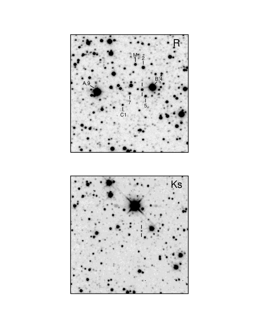
Figure 1: Top: 350 s $R$ band exposure of the field of GX 349+2 taken with the CTIO 0.9 m telescope. North is up and east is to the left; the field size is 2′$\times$2′. The designation of the objects follows Jernigan et al. (1978) and Penston et al. (1975) except for objects M and C1 which had no previous designations. The X-ray counterpart has also previously been called star 6. Bottom: Average of 15 60 s $Ks$ band exposures of the same field taken with the CTIO 1.5 m telescope. GX 349+2 is marked.

Since previous finding charts of GX 349+2, obtained with photographic plates, are of modest quality, a CCD image of the field is displayed in the top panel of Figure 1. GX 349+2 and all comparison stars used in the analysis are marked. Due to the crowded field, aperture photometry is not possible, and all photometry was performed by point spread function fitting with DAOPHOT II (Stetson 1993). The instrumental magnitudes were transformed to the standard system through observations of several Landolt standard star fields (Landolt 1992) obtained on two of the nights during the observing run. The mean magnitudes of GX 349+2 (averaged over the whole observing run) and several local comparison stars are listed in Table 2.1. The systematic error (from the transformation to the standard system) in these optical magnitudes is $\pm 0.04$ mag. The intrinsic 1$\sigma$ error of the relative photometry is $\pm 0.01$ mag, derived from the rms scatter of the comparison lightcurve (see Figure 2). Previous individual photometric measurements by Cooke & Ponman (1991) resulted in $B=20.2$ and $V=18.7$. Their measurements were not taken under photometric conditions and instead stars A and B (which had been measured by Penston et al. 1975) were used as secondary standards. Similar observations by Penninx & Augusteijn (1991) gave $B=20.0\pm 0.1$ and $V=18.4\pm 0.1$. Our $V$ magnitude of $18.56\pm 0.04$ agrees with these earlier measurements; there are no previous R band measurements with which to compare our results.

2.2 Near-infrared Photometry

In addition to the optical photometry, near-infrared (IR) $JHK$ and $Ks$ photometry of GX 349+2 was performed with the Cerro Tololo Infrared Imager (CIRIM) on the CTIO 1.5 m telescope on 1995 June 5 and 6 UT. CIRIM uses a 256$\times$256 HgCdTe NICMOS3 array. All observations were taken in the $f/13.5$ mode resulting in a pixel scale of $0.65\arcsec$ pix^-1. Four 15 s exposures were coadded to obtain one exposure. Each observation consisted of a mosaic of nine individual frames, with each frame shifted from the previous one by $20\arcsec$ to form a 3$\times$3 grid centered on the position of GX 349+2. Dark frames with identical integration times and flat field frames for each filter (derived from observations of an illuminated dome spot) were obtained on each night. First, a mean dark frame was subtracted from all observations. Next, a sky flat was constructed from a median of the scaled object frames and subtracted from each observation. Finally, the data were divided by the normalized dome flat. To increase the signal-to-noise and eliminate bad pixels, several of the shifted frames were aligned and combined with a bad pixel mask. A $Ks$ frame at the same scale as the optical image is displayed on the bottom panel of Figure 1 for comparison. Notice the impressive increase in the brightness of star M between the $R$ and the IR image. This star is not visible on our $V$ frame, has $R=17.2\pm 0.1$, and is saturated on our $J$, $H$ and $K$ frames. Star M was reported to be variable and briefly considered as the optical counterpart for GX 349+2 (Zuiderwijk 1978, Glass & Feast 1978), but was subsequently shown to probably be a Mira variable (Glass 1979).

Again, photometry was performed by point spread function fitting with DAOPHOT II. The instrumental magnitudes were transformed to the standard system (CIT) through observations of Elias faint infrared standards (Elias et al. 1982). The results for GX 349+2 and several local comparison stars are listed in Table 2.1. The systematic errors in the IR photometry are rather large ($\pm 0.2$ mag) due to only partially photometric observing conditions. Furthermore, the transformation to the standard system was accomplished simply by a zero point offset, neglecting color effects. Cooke & Ponman (1991) obtained a low spatial resolution map at $H$ and derive a magnitude of H$\approx$15. Our $H$ magnitude of $14.5\pm 0.2$ is probably consistent with that measurement (for which no errors are given).

3 Results

The $R$ band lightcurves for GX 349+2 and a slightly fainter comparison star (star 5) are displayed in Figure 2. The magnitude of the comparison lightcurve has been shifted to brighter magnitudes by 0.6 mag to separate the two curves for display purposes. The systematic errors from the transformation to the standard system are not included in the error bar. The differential lightcurve of GX 349+2 clearly displays variability of up to 0.3 mag during a single night. This marked intraday variability may be added to the positional coincidence with the radio source and the observed H$\alpha$ emission to conclude with confidence that the correct optical counterpart to the X-ray source has been identified.

The data were searched for periodic behavior with a power spectrum analysis using the CLEAN algorithm (Roberts et al. 1987). Figure 3 shows the “dirty” spectrum, the power spectrum created by the sampling window, and the cleaned spectrum after 20 iterations of CLEAN with a gain of 0.2. The cleaned power spectrum exhibits a strong peak around $\sim$21.4 h. An analytic assessment of the statistical significance of the peak is complicated by the markedly nonuniform sampling of the data, and the repeated application of the CLEAN algorithm. We prefer instead a Monte Carlo simulation with boundary conditions that accurately mimic the actual data. To this end we have scrambled the vectors of time vs. magnitude with a random number generator, thereby creating nonsense data with the identical sample times (and thus window function) and standard deviation as the real data. These randomized data were then CLEANed and transformed in the identical way as the actual observations, and the resulting power spectrum was examined for peaks. In 100 iterations of this scrambling process, none of the resulting power spectra contained any peak at any frequency of height as significant as the signal observed in the actual data. We conclude that the dominant peak is statistically significant with at least 99% confidence.

In order to test the reliability of the peak position, the dirty spectrum was cleaned with a range of gain values and number of CLEAN iterations, and the resultant peak was fitted with a Gaussian. The peak center varied between 1.29$\times 10^{-5}$ s^-1 (21.53 h) and 1.31$\times 10^{-5}$ s^-1 (21.20 h); the typical HWHM of the peak is 1.35 h. Since the power spectrum peak is so broad ($\pm 0.9$ h lies within the width of one phase bin on either side of the peak center), and it is known that CLEAN can shift the peak center frequencies in the presence of noise (Carbonell et al. 1992), we searched the period range 19.0 h to 23.5 h by folding the data on a given period in steps of 0.1 h and fitting a sine wave. The period with the smallest rms after subtraction of the best fit is 21.85 h. In order to arrive at an error estimate for this period we performed Monte Carlo simulations. The best sine fit for the period of 21.85 h was subtracted from the data, and the resulting residuals scrambled and added back into the data. Then the process of folding and fitting the data was repeated. The resulting distribution of periods after 1000 iterations of this process gives a 1$\sigma$ error of 0.13 h. We adopt 21.85$\pm 0.4$ h for the best period and 3$\sigma$ error.

Figure 4 shows the photometric data folded on the best period of 21.85 h. The best-fitting sine wave has been overplotted, and two cycles are shown for clarity. The sine fit gives a half-amplitude of 0.14 mag for the variations.

The folded lightcurve of GX 349+2 shows that the periodic variation is superposed on erratic flickering. This is not surprising, as both of the other photometrically observed Z-sources, Sco X-1 and Cyg X-2, also show large scatter in their lightcurves (Goranskii & Lyutyi 1988, Augusteijn et al. 1992). However, caution will be needed to insure that the variations seen in GX 349+2 are truly periodic and not simply due to random variability observed over a relatively short time span. Additional observations will test the reliability of this period. It is interesting to note that van Paradijs & McClintock (1994) predict a period between 3 and 52 h for GX 349+2 from a relationship between the absolute visual magnitude, the X-ray luminosity, and the period of a LMXB system.

We have searched for an analog of the 21.85 h period in the X-ray emission from GX349+2, using the preliminary public version of the All Sky Monitor data from the Rossi X-ray Timing Explorer (quick-look results provided by the ASM/RXTE team, http://space.mit.edu/XTE/asmlc/ASM.html). No such periodic behavior is evident, using a variety of analysis techniques. Although the X-ray data are well-sampled, in these observations the source is highly and chaotically variable on a timescale of hours, with typical amplitudes of 30%, thereby leading to relatively uninteresting upper limits on any periodic behavior.

Brightness variations in LMXBs can have several different origins, e.g., X-ray heating of part of the surface of the secondary, ellipsoidal distortion of the companion due to the gravitational influence of the compact object, a “hot spot” on the edge of the accretion disk, the accretion stream, or a combination of these effects. It is difficult to distinguish between these different possibilities merely on the basis of photometric data. For ellipsoidal variations a double peaked lightcurve is expected, while in the other cases a single peaked lightcurve is seen. As a consequence, our period could be either the orbital period or half the orbital period. This ambiguity can only be resolved through radial velocity measurements.

Ellipsoidal variations are usually observed in LMXB systems where the secondary contributes significantly to the observed light, and stellar features of the secondary are seen in the spectrum of the system (e.g., Cyg X-2, Cowley et al. 1979). No underlying stellar features are visible in the spectrum of GX 349+2 published by Penninx and Augusteijn (1991). Unfortunately, the spectrum is of rather low quality and those authors caution that they would have been unable to detect stellar features of the strength seen in Cyg X-2. The amplitude of ellipsoidal variations is usually small, $\lesssim 0.1$ mag full amplitude, in comparison to which the full amplitude of variations in GX 349+2 (0.28 mag) seems fairly large. Yet, Cyg X-2 shows a double peaked lightcurve due to ellipsoidal variations with a full amplitude of 0.25 mag in the $B$ band; therefore this explanation still seems viable for GX 349+2.

On the other hand, Sco X-1 shows a single peaked lightcurve (Augusteijn et al. 1992) over its period, and due to the similarity between Sco X-1 and GX 349+2 in the X-ray regime, one might expect that the intrinsic properties of their optical counterparts would also resemble each other. Note that if our period reflects the orbital period of the system, then the periods of Sco X-1 and GX 349+2 are quite similar. The optical variability of Sco X-1 is thought to be due to X-ray heating of the disk and/or secondary. In the case of X-ray heating of the secondary, large amplitude variations are expected over the orbit (e.g., $\sim$1.5 mag in the Her X-1 system). The fact that only small amplitude variations (0.13 mag full amplitude, Augusteijn et al. 1992) are seen in Sco X-1 has been attributed to a low system inclination. If the GX 349+2 variations are also due to X-ray heating of the secondary, it might also imply a low inclination for this system. Support for GX 349+2 being a moderate to low inclination system comes from the fact that no X-ray eclipses have been reported so far. Furthermore, Kuulkers (1995) suggested that some intrinsic differences in the X-ray properties among the Z-sources are due to inclination effects. He groups GX 349+2 with Sco X-1 and GX 17+2 as basically face-on systems. The determination of the inclination is extremely important since this is of course one of the parameters that enters into the calculation of the component masses. Modeling of the photometric lightcurve, once the period is confirmed and the phase coverage of the lightcurve is complete, might be valuable in this respect. For the following discussion we assume that the observed variability is not due to ellipsoidal variations, but that 21.85 h is the actual orbital period of the system.

4 Discussion

Recently, Southwell et al. (1996) suggested a period of 14 d for GX 349+2 from an analysis of the H${\alpha}$ emission line velocities. However, their data are sampled extremely sparsely and not at the comparatively short timescale of our period. There is no obvious alias relationship between the candidate spectroscopic and photometric periods. If the Southwell et al. observations define the true radial velocity semi-amplitude of the system ($K\approx 70$ km s^-1) but our photometric period is the actual orbital period, then the implied mass function is $f(M)=0.032$ M_☉; however, both of these assumptions are currently uncertain. By comparison, the mass function for Sco X-1 is $f(M)=0.016$ M_☉ (Cowley & Crampton 1975), a similarly small value. The period of Southwell et al. (1996) would imply $f(M)=0.5$ M_☉.

If the H${\alpha}$ emission arises in the accretion disk, then the observed velocity is indicative of the neutron star; if instead the emission originates from the X-ray heated side of the secondary, then the radial velocity traces the motion of the optical companion. This question can ultimately only be answered by simultaneous spectroscopy and photometry to determine the location of the emitting region. With our (highly uncertain) mass function of $f(M)=0.032$ M_☉, we can derive the component masses and Roche lobe size of the secondary for a given inclination $i$ and mass ratio $q=M_{2}/M_{1}$, where $M_{2}$ refers to the optical (mass donor) companion. Various curves of constant inclination and mass ratio are shown in Figure 5 (calculated under the assumption that the H${\alpha}$ emission arises in the accretion disk). Assuming a mass for the neutron star of $M_{1}\leq 2$ M_☉, we see that for $i\gtrsim 25^{\arcdeg}$ the mass of the companion is $M_{2}<2$ M_☉. For $i\lesssim 15^{\arcdeg}$ the companion is more massive than the neutron star. We can calculate the binary separation $a$ for a given neutron star mass and mass ratio from Kepler’s law:

$$a=3.5\times 10^{10}~{}(M_{1}/M_{\sun})^{1/3}~{}(1+q)^{1/3}~{}P_{h}^{2/3}{\rm cm}$$ (1)

The Roche lobe radius of the companion for a given $q$ is then obtained from the approximate analytic formula of Eggleton (1983)

$$\frac{R_{L}}{a}=\frac{0.49q^{2/3}}{0.6q^{2/3}+ln(1+q)^{1/3}}$$ (2)

A sample list of binary separation, Roche lobe radius and main sequence star radius of the corresponding $q$ is given in Table 4. We see that for up to very high mass ratios, the Roche lobe of the secondary is too large to be filled by a main sequence star with the appropriate mass. Therefore, for mass transfer to occur, the companion must be slightly evolved. These conclusions are almost identical to those reached for Sco X-1 by Cowley & Crampton (1975).

We can also attempt to derive clues to the nature of the secondary from the photometry of GX 349+2, especially from the IR magnitudes. Photometry in the IR has certain advantages over optical photometry in determining the spectral type and luminosity class for this object. First, the extinction in the IR is much smaller ($A_{K}/A_{V}=0.114$, Cardelli et al. 1989), thereby reducing the relative size of any error in the extinction estimate. Also, most LMXBs are dominated by the light from the accretion disk in the optical. Since the energy distribution of an accretion disk peaks in the blue, it is expected that contamination by the disk diminishes towards longer wavelengths, so that the companion should be more easily observed. As a caveat to this statement, we note that Cowley et al. (1991) conducted a spectroscopic survey of LMXBs in the near-IR (8000–9000 Å) and find that in most systems the accretion disk emission still dominates the spectrum. Observations of cataclysmic variables showed that the disk contribution in the IR varies from case to case, with several systems still indicating a strong contribution of light from the accretion disk (Berriman et al. 1985, Friend et al. 1988).

The extinction for GX 349+2 has been estimated from various methods to lie between $A_{V}=$4–6 mag (Penninx & Augustijn 1991, Cooke & Ponman 1991). Adopting $A_{V}=5$ mag, we arrive at dereddened magnitudes of $J=13.6$, $H=13.55$, and $K=14.0$ for GX 349+2. Distance estimates for GX 349+2 range from 8.5 kpc (canonical distance to the Galactic Center, Cooke & Ponman 1991) to 10 kpc (assuming that Z-sources radiate with the Eddington luminosity in X-rays, van Paradijs & McClintock, 1994). This results in an absolute $K$ magnitude of $M_{K}=-0.6$ or $M_{K}=-1.0$, respectively. These magnitudes correspond to a main sequence spectral type of roughly B5, but the $(J-K)_{0}$ color is then too blue by 0.28 mag. Although this would still be within our photometric errors, it seems unlikely that GX 349+2 has a B5 main sequence star companion. A B5 companion would account for all the light seen in the $B$ and $V$ band and therefore exclude the presence of an accretion disk. This would make GX 349+2 a high mass X-ray binary system, which seems inconsistent with its X-ray properties. It is more likely that the accretion disk still contributes considerable flux in the IR and that the IR colors are not necessarily indicative of the companion.

5 Conclusions

We have carried out the first photometric study of the optical counterpart of the Z-source GX 349+2. We find variability of 0.3 mag during a single night and a significant $21.85$ h period superposed on erratic flickering. Assuming this to be the orbital period of the system together with a velocity amplitude reported by Southwell et al. (1996), we find a mass function quite similar to that of Sco X-1. Infrared photometry seems to indicate that the disk is still contributing considerable flux in the $K$ band.

Table 1: Z-sources

X-ray Source	Alternate Name	Optical Cpt.	$V$	Period (h)
Sco X-1	1617$-$155	V818 Sco	12.2	18.90
GX 340+0	1642$-$455	$\cdots$	$\cdots$	$\cdots$
GX 349+2	1702$-$363	star 6	18.6	21.85 /334.6
GX 5-1	1758$-$250	$\cdots$	$\cdots$	$\cdots$
GX 17+2	1813$-$140	NP Ser	17.5	$\cdots$
Cyg X-2	2142$+$380	V1341 Cyg	14.7	236.2

Table 2: Magnitudes of GX 349+2 and comparison stars

Object	$V$	$R$	$J$	$H$	$K$
GX 349+2	18.56	17.55	15.0	14.5	14.6
5	19.23	17.76	$\cdots$	13.1	13.1
2	17.99	16.61	$\cdots$	$\cdots$	$\cdots$
7	19.46	17.99	14.3	13.3	13.2
C1	19.96	18.34	14.5	13.4	13.3

Table 3: Parameters of GX 349+2

$q$	$a$ $(R_{\sun})$	$R_{L}(M_{2})$$(R_{\sun})$	$R_{MS}(M_{2})$ $(R_{\sun})$
0.1	4.49	0.93	0.25
0.3	4.75	1.33	0.54
0.5	4.98	1.60	0.78
0.7	5.19	1.81	0.98
1.0	5.48	2.08	1.27
1.5	5.91	2.45	1.68
2.0	6.28	2.76	2.06
2.5	6.61	3.04	2.40
3.0	6.91	3.29	2.73
3.5	7.18	3.52	3.04
4.0	7.44	3.73	3.34

Figure 2: Lightcurve of GX 349+2 and a comparison star of similar brightness. The magnitudes of comparison star 5 have been shifted to brighter magnitude by 0.6 mag for clarity of display. The representative 1$\sigma$ error bar has been obtained from the rms scatter in the differential lightcurve of the two comparison stars.

Figure 3: Power spectrum analysis with the CLEAN algorithm. Top panel: the “dirty” spectrum, i.e., the convolution of the periodicities in the observed data with the sampling window; middle panel: the sampling window; lower panel: the cleaned spectrum after 20 iterations with a gain of 0.2. The highly significant peak at $\sim$21.4 h is clearly visible. The next strongest peak, near 50 h, is not statistically significant.

Figure 4: The lightcurve for our photometric data of GX 349+2, folded on the best period of 21.85 h. Also plotted is the best-fitting sine wave. Two cycles are shown for clarity.

Figure 5: Possible masses for the components in GX 349+2, adopting a mass function $f(M)=(M_{2}sini)^{3}/(M_{1}+M_{2})^{2}=0.032$ M_☉. Curves of constant inclination (solid) and constant mass ratio (dashed) are labeled.

References

- (1) Augusteijn, T. et al. 1992, A&A, 265, 177
- (2)
- (3) Berriman, G., Szkody, P., & Capps, R. W. 1985, MNRAS, 217, 327
- (4)
- (5) Carbonell, M., Oliver, R., & Ballester, J. L. 1992, A&A, 264, 350
- (6)
- (7) Cardelli, J. A., Clayton, G. C., & Mathis, J. S. 1989, ApJ, 345, 245
- (8)
- (9) Cooke, B. A., & Ponman, T. J. 1991, A&A, 244, 358
- (10)
- (11) Cowley, A. P., & Crampton, D. 1975, ApJ, 201, L65
- (12)
- (13) Cowley, A. P., Crampton, D., & Hutchings, J. B. 1979, ApJ, 231, 539
- (14)
- (15) Cowley, A. P., Schmidtke, P. C., Crampton, D., Hutchings, J. B., & Bolte, M. 1991, ApJ, 373, 228
- (16)
- (17) Deutsch, E. W., Margon, B., Wachter, S. & Anderson, S. F. 1996, ApJ, 471, in press
- (18)
- (19) Eggleton, P. P. 1983, ApJ, 268, 368
- (20)
- (21) Elias, J. H., Frogel, J. A., Matthews, K., & Neugebauer, G. 1982, AJ, 87, 1029
- (22)
- (23) Friend, M. T., Martin, J. S., Smith, R. C., & Jones, D. H. P. 1988, MNRAS, 233, 451
- (24)
- (25) Glass, I. S. 1979, MNRAS, 187, 807
- (26)
- (27) Glass, I. S., & Feast, M. W. 1978, IAU Circ. 3226
- (28)
- (29) Goranskii, V. P., & Lyutyi, V. M. 1988, Sov. Astron., 32(2), 193
- (30)
- (31) Hasinger, G., & van der Klis, M. 1989, A&A, 225, 79
- (32)
- (33) Jernigan, J. G., Apparao, K. M. V., Bradt, H. V., Doxsey, R. E., Dower, R. G., & McClintock, J. E. 1978, Nature, 272, 701
- (34)
- (35) Kuulkers, E. 1995, PhD thesis, University of Amsterdam
- (36)
- (37) Landolt, A. U. 1992, AJ, 104, 340
- (38)
- (39) Lewin, W. H. G., & van Paradijs, J., 1985, A&A, 149, L27
- (40)
- (41) Miller, B. W., Margon, B., & Burton, M. G. 1993, AJ, 106, 28
- (42)
- (43) Penninx, W., & Augusteijn, T. 1991, A&A, 246, L81
- (44)
- (45) Penston, M. V., Penston, M. J., Murdin, P., & Martin, W. L. 1975, MNRAS, 172, 313
- (46)
- (47) Ponman, T., J., Cooke, B. A., & Stella, L. 1988, MNRAS, 231, 999
- (48)
- (49) Roberts, D. H., Lehar, J., & Dreher, J. W. 1987, AJ, 93, 968
- (50)
- (51) Schulz, N. S., Hasinger, G., & Trümper, J. 1989, A&A, 225, 48
- (52)
- (53) Southwell, K. A., Casares, J., & Charles, P. A. 1996, in Cataclysmic Variables and Related Objects, IAU Colloq. 158, A. Evans & J. H. Wood (eds.) (Dordrecht: Kluwer), in press
- (54)
- (55) Stetson, P. B. 1993, DAOPHOT II User’s Manual
- (56)
- (57) van Paradijs, J., & McClintock, J. E. 1994, A&A, 290, 133
- (58)
- (59) van Paradijs, J. 1995, in X-Ray Binaries, W. H. G. Lewin, J. van Paradijs, & E. P. J. van den Heuvel (eds.) (Cambridge: Cambridge Univ. Press), p. 536
- (60)
- (61) Vrtilek, S. D., McClintock, J. E., Seward, F.D., Kahn, S. M., & Wargelin B. J. 1991, ApJS, 76, 1127
- (62)
- (63) Zuiderwijk, E. J. 1978, IAU Circ. 3221
- (64)