A catalogue of the voids in the IRAS 1.2-Jy survey

Abstract

Using the void finder algorithm we have compiled a catalogue of voids in the IRAS 1.2-Jy sample. The positions of the voids correspond well to the underdense regions seen in the IRAS smoothed density map. However, since in our analysis no smoothing is used, all structures appear much sharper: walls are not smeared and the voids are not artificially reduced by them. Therefore the current method based on the point distribution of galaxies is better suited to determine the diameter of voids in the galaxy distribution. We have identified 24 voids, covering more than 30 per cent of the volume considered. By comparing the results with equivalent random catalogues we have determined that 12 voids are significant at a $0.95$ confidence level, having an average diameter of $40\pm 6h^{-1}\,\mbox{Mpc}$. Our results serve not only for charting the cosmography of the nearby Universe, but also to give support to the results recently obtained with the SSRS2 sample, suggesting a void-filled Universe. Moreover, our results indicate that the voids detected have a similar scale, demonstrating that both optically selected and IRAS-selected galaxies delineate the same large-scale structures.

1 Introduction

A remarkable feature of the distribution of galaxies is the existence of large regions apparently devoid of luminous matter. Since the discovery of the Boötes void [Kirshner et al. 1981] it was realized that the existence of large voids in the galaxy distribution could impose additional constraints to models of large-scale structure (LSS). Since then complete surveys like the CfA2 [Geller & Huchra 1989] and SSRS2 [da Costa et al. 1994], which densely sample the nearby galaxy distribution, have shown that voids are a major feature of the LSS. These surveys show that not only large voids exist, but more importantly – that they occur frequently (at least judging by eye), suggesting a compact network of voids filling the entire volume. The impact that these findings have in discriminating models for the origin of LSS has recently been addressed by Blumenthal et al. [Blumenthal et al. 1992], Dubinski et al. [Dubinski et al. 1993], Piran et al. [Piran et al. 1993] and van de Weygaert & van Kampen [van de Weygaert & van Kampen 1993].

As mentioned above, until recently the description of a void-filled Universe with a characteristic scale of $50h^{-1}\,\mbox{Mpc}$ relied solely on the visual impression of redshift maps. In order to make a more quantitative analysis we have developed an algorithm for the automatic detection of voids in three-dimensional surveys. The main features of the algorithm are as follows.

1. It is based on the point-distribution of galaxies, not introducing any smoothing scale which destroys the sharpness of the observed features.

2. It allows for a population of galaxies in voids, recognizing that voids need not be completely empty.

3. It tries to avoid the artificial connection between neighbouring voids through small breaches in the walls, realizing that walls in the galaxy distribution need not be homogeneous as small-scale clustering will always be present.

The method has been recently applied to the SSRS2 sample of galaxies [El-Ad, Piran & da Costa 1996, hereafter paper I]. Some 12 significant voids with density contrast $\sim-0.9$ were detected with an average diameter of $37\pm 8h^{-1}\,\mbox{Mpc}$ and comprising roughly 40 per cent of the surveyed volume, clearly supporting earlier qualitative claims. Unfortunately, the advantage of the dense sampling of the galaxy distribution attained with the SSRS2, which allows for a larger range of significant voids to be detected, is offset by the effects of the geometry of the survey.

In order to overcome this limitation we consider here the IRAS 1.2-Jy survey [Fisher et al. 1995]. Although much sparser than the optical surveys, the IRAS sample provides essentially a full sky coverage minimizing boundary effects. The trade-off is between boundary effects and the statistical significance of the voids. The IRAS data also provide a suitable bench mark as they have been used to derive the smoothed density field [Strauss & Willick 1995], and they probe a volume comparable to that used to determine the density field of the underlying mass distribution from reconstruction methods based on the measured galaxy peculiar velocity field (Dekel 1994, Freudling, da Costa & Pellegrini 1994, da Costa et al. 1996). Recently, Dekel et al. [Dekel et al. 1993] compared the density field recovered by the potent method with the smoothed density field of IRAS galaxies. Both of these fields will be used below (Section 5) to compare our results.

Earlier statistical works analysing the IRAS data (Fisher et al. 1995 and references therein) rarely addressed the voids. An exception are the works on the Void Probability Function (VPF): Bouchet et al. [Bouchet et al. 1993] calculated the VPF for various volume-limited IRAS subsamples; Watson & Rowan-Robinson [Watson & Rowan-Robinson 1993] incorporated into the VPF analysis the effects of the selection-function, and applied it to the one-in-six 0.6-Jy QDOT sample. Both works show how the VPF departs from Poisson statistics. In addition, several individual voids were pointed out within the IRAS sample (cf. the recent review by Strauss & Willick, chapter 4): among these were the Local Void [Tully 1987] and the Sculptor Void [da Costa et al. 1988]. However, no objective algorithm has ever been applied to compile a void catalogue for the whole survey.

We use here an improved version of the void finder algorithm (paper I), to compile a void catalogue for the IRAS survey. Our focus here is two-fold.

1. Cosmography of the nearby Universe: we chart the individual voids, objectively identified within a sphere of radius $80h^{-1}\,\mbox{Mpc}$, and compare this picture to the one depicted by other techniques.

2. Void statistics: we derive the average diameter and other properties of the significant voids, and compare them to those derived in paper I for the SSRS2. The possible implications regarding galaxy biasing are also discussed.

We review the void finder algorithm in Section 2. The sample we use is presented in Section 3. In Section 4 we give a pictorial description of the void distribution, and describe the statistical properties of the voids that we measure. In Section 5 we compare several reconstruction methods, and discuss the implications of our results. Finally, a summary of our main conclusions is presented in Section 6.

2 The VOID FINDER algorithm

Since the void finder algorithm used for the IRAS data is a somewhat improved version of the one used in paper I for the analysis of the SSRS2, we include here a description of the updated algorithm. A complete description can be found in El-Ad & Piran [El-Ad & Piran 1997]. The algorithm is based on a model in which the main features of the LSS of the Universe are voids and walls. The walls are thin structures characterized by a high density of galaxies, separating the voids. These are underdense regions, but are not completely empty, being populated by a relatively small number of void galaxies.

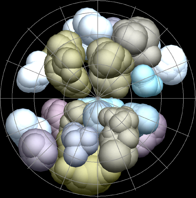
Figure 2: Three-dimensional view of the voids in the IRAS survey. All 24 voids are included in this image. The ZOA runs horizontally across the image. The area at the left, near the ZOA, with no voids, corresponds to the Great Attractor. The absence of voids from the lower, right-hand part of the image is due to the Cetus wall and the PP supercluster. 3D graphics by Shai Ayal.

The void finder algorithm initially locates the voids containing the largest empty spheres. Following iterations locate the smaller voids, and – when appropriate – enlarge the volumes of the older voids. This identification scheme implies the following definition for a void: it is a continuous volume that does not contain any (wall) galaxies, and is thicker than an adjustable limit. Spheres that are devoid of galaxies are used as building blocks for the voids. A single void is composed of as many superimposing spheres as required for covering all of its volume. The algorithm is iterative, with subsequent iterations searching for voids using a finer void resolution, which is defined as the diameter $d_{i}$ of the minimal sphere used for encompassing a void during the $i$th iteration. The spheres for covering a void are picked up in two stages: the identification stage, followed by consecutive enhancements. We will now describe these stages in detail.

The identification stage identifies the central parts of the void. Usually, this is enough for covering about half of the actual volume, but we focus (at this stage) on identifying a certain void as a separate entity, rather than trying to capture all of its volume. The central parts of a void are covered using spheres with diameters in the range $\xi d_{\mathrm{max}}<d\leq d_{\mathrm{max}}$, with $d_{\mathrm{max}}$ denoting the diameter of the largest sphere of a void and $\xi$ being the thinness parameter. The thinness parameter controls the flexibility allowed while encompassing the central parts of a void. Setting $\xi=1$ would leave us with only the largest sphere in the void, while lowering $\xi$ allows the addition of more spheres. If the void is composed of more than one sphere (as is usually the case), then each sphere must intersect at least one other sphere with a circle wider than the minimal diameter $\xi d_{\mathrm{max}}$. We have taken $\xi=0.85$, which allows for enough flexibility – still without accepting counter-intuitive void shapes. A lower $\xi$ reduces the total number of the voids, with a slow increase in their total volume. Once a group of such intersecting spheres has been dubbed a void, it will not be merged with any other group.

After the central part of a void is identified, we consecutively enhance its volume, in order to cover as much of the void volume as possible using the current void resolution. These additional spheres need not adhere to the $\xi$ thinness limitation: during each subsequent iteration, we scan the immediate surroundings of each of the voids already identified. If we find additional empty spheres that intersect with the void, then these are added to the void. We scan for enhancing spheres of a certain diameter only after scanning for new voids with that diameter. In this way we do not falsely break apart individual voids, and we do not prevent the identification of truly new voids.

Since the average galaxy number density decreases with depth, as only the brighter galaxies are observable at greater distances, we must apply corrections to the algorithm in order to minimize these effects. The correction used by the void finder is to scale the diameters of the spheres by the selection function, thus accepting only relatively larger spheres in the sparser regions of the survey.

The full algorithm includes also a pre-selection stage – the wall builder – that identifies wall galaxies (which are used later to define the voids) and field galaxies (which are ignored). However, since the IRAS sample is relatively sparse, we have taken a more conservative approach, and considered all the galaxies while identifying the voids. Hence, the IRAS voids presented below are completely empty. Comparison of these results with voids found after filtering field galaxies indicates that the filtering process affects the cosmography (some voids are merged), but it has only a small effect on the void statistics (see Section 4).

We define a wall galaxy as a galaxy that has at least $n$ other wall galaxies within a sphere of radius $\ell_{n}$ around it. The radius $\ell_{n}$ is derived based on the statistics of the distance to the $n$th nearest neighbour. In our analysis we use $n=3$. The wall builder corrects for the selection function in a similar way to the void finder: we determine $\ell_{3}$ in the volume-limited region of the sample (see below), beyond which we scale it by the selection function.

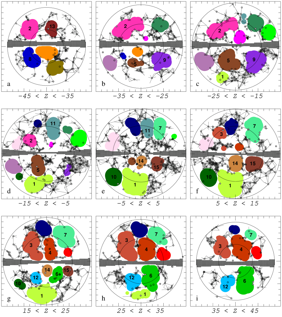
Figure 4: IRAS voids and walls in slices parallel to the SG plane. The shaded areas mark the intersection of the centre of the given plane with the three-dimensional voids. Darker shading implies a more significant void. Only the fifteen $p>0.8$ voids are numbered (see Table 2). The excluded ZOA is indicated along $Y=0$. The depicted galaxies extend $5h^{-1}\,\mbox{Mpc}$ above and below the plane. Wall galaxies are marked as by ‘$\circ$’, and field galaxies by ‘$\oplus$’. Note that all the galaxies are located outside the voids – galaxies that seem to be in a void appear so due to the two-dimensional projection. As a visual aid for highlighting the walls, we have drawn lines connecting between all pairs of wall galaxies closer than the properly scaled wall separation distance $\ell_{3}$. These artificial connections are not used in our analysis. If the SGZ plane drawn is perpendicular to a wall, we see a thin dense feature – e.g., as seen in panel (h). If the projection plane coincides with a plane of a wall, we see a wide dense feature. This is evident in the SG plane (panel e), where the Cetus wall and PP occupy a large fraction of the slice. The inner circle at $r_{o}=50h^{-1}\,\mbox{Mpc}$ marks the volume-limited region of our sample. The outer circle marks the boundary of the sample, at $r_{\mathrm{max}}=80h^{-1}\,\mbox{Mpc}$.

3 The sample

The IRAS survey contains 5321 galaxies complete to a flux limit of 1.2-Jy [Fisher et al. 1995]. We applied corrections for the computed peculiar velocities, to obtain the real-space distribution of the galaxies. In the void analysis, we have limited ourselves to galaxies extending out to $r_{\mathrm{max}}=80h^{-1}\,\mbox{Mpc}$, and created a semi–volume-limited sample consisting of galaxies brighter than $l_{60}\geq 3.59\times 10^{30}h^{-2}{\mathrm{erg\,s}}^{-1}{\mathrm{Hz}}^{-1}$ at $60\mu\mathrm{m}$, corresponding to a depth $r_{o}=50h^{-1}\,\mbox{Mpc}$. The selection function $\phi$ drops to 22 per cent at $r_{\mathrm{max}}$. The final sample consists of 1876 galaxies. The 1531 faint galaxies that were eliminated in order to create the volume-limited region of the survey are not used when processing the walls nor the voids. However, after the survey is analysed and the voids located, we examine the locations of these faint galaxies (see Section 4.2).

The sky coverage of the IRAS is almost complete ($87.6$ per cent), with the galactic plane region $|b|<5\hbox{${}^{\circ}$}$ constituting most of the excluded zones. Various schemes (e.g., that of Yahil et al. 1991) have been used to extrapolate the density field to the Galactic plane, but these are not directly applicable to our analysis. Thus, when looking for voids we avoid the zone of avoidance (ZOA), treating it as a rigid boundary practically cutting the IRAS sample into two halves. Since the ZOA cuts across voids this scheme divides some voids to two and eliminates others. However, it is the most conservative method, and therefore the results for the volumes of the voids should be considered as lower limits. We estimate the effect of this method by examining the opposite approach in which the ZOA is treated as if it is a part of the survey, applying no corrections. The ZOA is nowhere wider than the minimal void resolution used, so it does not create new voids by itself. Therefore the effect of including the ZOA is to overestimate the size of voids near it, because it allows the merging of a couple of voids and the expansion of other voids into the region. Still the overall effect on the void statistics is limited (see Section 4.2).

Areas lacking sky coverage in the Point Source Catalog constitute most of the remaining excluded zones. These were processed as if they were included in the IRAS, as their effect is rather negligible. However, when the voids we find include these regions, that is indicated (see Section 4.1).

The wall builder analysis of the IRAS galaxy distribution located 95 per cent of the galaxies within walls. Each wall galaxy was required to have at least three other wall galaxies within a sphere of radius $\ell_{3}=10.2h^{-1}\,\mbox{Mpc}$ around it. We find that the walls occupy at most $\sim 25$ per cent of the examined volume. This corresponds to an average wall overdensity of at least $\delta\rho/\rho\approx 4$. Note that here we have used a sample somewhat deeper than $r_{\mathrm{max}}$ so galaxies located near the boundary of our sample are not mistakenly recognized as field galaxies.

4 The IRAS voids

4.1 Cosmography

Applying our most conservative approach to analyse the IRAS data – i.e., including the field galaxies and avoiding the ZOA – we have identified 24 voids of which 12 are statistically significant at a $0.95$ confidence level (see Section 4.2). Fig. 2 depicts a three-dimensional view of the IRAS voids. Fig. 4 shows the voids and the walls, in nine planes parallel to the supergalactic (SG) plane at $10h^{-1}\,\mbox{Mpc}$ intervals. In general, some of the voids shown are smaller than their actual size – because of the way we treat the ZOA, or because the field galaxies were not removed from the analysis. Both effects imply that our estimates of the size of voids are likely to be lower limits.

In the SG plane (Fig. 4, panel e) one recognizes void 10 as the Sculptor Void [da Costa et al. 1988], located below the Pavo–Indus–Telescopium part ($Y<0$) of the Great Attractor (GA), seen here to be composed of several substructures. Adjacent to it we find void 1, stretching parallel to the Cetus wall. These two voids are separated only by a few field galaxies. If we filter them out, the two would merge to form one huge void, equivalent in volume to a $d=62h^{-1}\,\mbox{Mpc}$ sphere occupying most of that part of the skies. Voids 1 and 10 are limited by the $r_{\mathrm{max}}$ boundary of our sample, so they could prove to be larger still.

The area above the Perseus–Pisces (PP) supercluster (up to the Great Wall near Coma, at $Y=70h^{-1}\,\mbox{Mpc}$) is occupied by two voids: 7 and 11. If the field galaxies are filtered first, these two voids merge. Also note in this area the minor void ($p=0.21$) located below the Coma supercluster, at $(X=-7,Y=54)$: this void (extending to the $Z>0$ panels) corresponds to the largest void found in the CfA survey [de Lapparent, Geller & Huchra 1986].

The closest void we found (void 14) can be seen in the centre of this panel, just below the Local Supercluster. Another clear, and rather nearby, void in the SG plane is void 15, in front of PP. A minor void can be viewed beyond the $Y>0$ section of the GA, at $(X=-51,Y=19)$.

Above the SG plane (Fig. 4, panels f–i) we see the extensions of the SG plane voids, as well as some additional voids – voids 3, 4, 6 and 12. Void 4 is the Local Void [Tully 1987]. Below the SG plane (Fig. 4, panels a–d) we note void 2 (just above the Hydra–Centaurus supercluster), and voids 5 and 9. Voids 8 and 13 extend around $Z=-40$ and can be seen in panel (a). We should point out that voids 1, 2, 5, 6, 7, 11 and 14 include areas lacking sky coverage in the PSC.

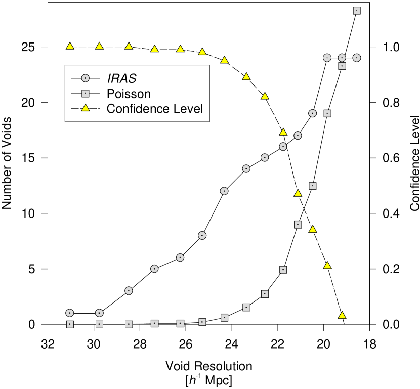
Figure 6: The accumulated number of voids as a function of the void resolution, for the IRAS sample and for random catalogues. The derived confidence level $p$ is also indicated.

Table 2: Locations and properties of the voids in the IRAS survey.

	Statistical	Equivalent	Total	Location of Centre				Largest
	Confidence	Diameter	Volume	(Supergalactic coordinates)				Sphere’s	Identification
	Level	[$h^{-1}\,\mbox{Mpc}$]	[$h^{-3}\,\mbox{KMpc}^{3}$]	$r$	$X$	$Y$	$Z$	Fraction
	(1)	(2)	(3)	(4)	(5)	(6)	(7)	(8)	(9)
1	$>$0.99	51.0	69.9	55.2	-10.7	-53.8	6.1	0.34
2	$>$0.99	43.8	44.4	49.6	-25.3	31.4	-28.9	0.33
3	$>$0.99	44.5	45.9	46.0	-24.8	26.7	28.1	0.28
4	$>$0.99	45.0	47.4	46.5	8.7	24.7	38.4	0.25	Local Void
5	$>$0.99	36.0	24.4	32.0	-13.0	-23.9	-16.9	0.46
6	$>$0.99	41.4	37.3	51.5	17.0	-32.2	36.4	0.30
7	$>$0.98	43.5	43.3	57.1	31.2	44.9	16.5	0.31
8	$>$0.98	39.5	32.6	60.4	-25.8	-22.7	-49.7	0.50
9	$>$0.95	36.0	24.4	49.8	35.9	-25.6	-23.0	0.35
10	$>$0.95	33.6	19.9	63.3	-48.0	-40.9	6.0	0.81	Sculptor Void
11	$>$0.95	32.0	17.2	48.6	11.8	46.6	-6.9	0.52
12	$>$0.95	31.5	16.5	49.9	-15.6	-35.7	31.3	0.46
13	$>$0.89	40.3	34.5	62.8	14.2	29.3	-53.7	0.47
14	$>$0.89	28.8	12.7	19.0	0.7	-16.4	9.6	0.58
15	$>$0.82	30.4	14.6	37.6	32.4	-17.0	8.6	0.42	Perseus–Pisces Void

a

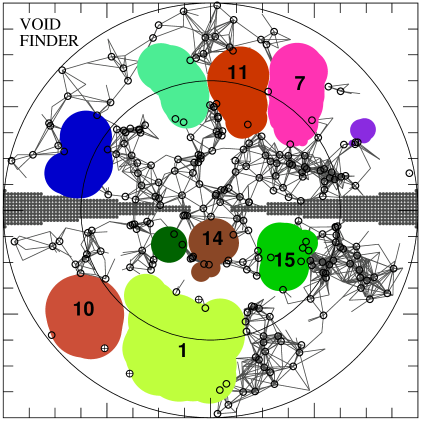
b

c

d

Figure 8: The supergalactic plane extending out to $80h^{-1}\,\mbox{Mpc}$, as depicted by various techniques. Panel (a): the locations of the voids and the walls, using the void finder algorithm. See the caption of Fig. 4 for details. Panel (b) (Strauss & Willick 1995): the real-space smoothed density field of IRAS galaxies, using $5h^{-1}\,\mbox{Mpc}$ Gaussian smoothing, extrapolating into the ZOA. The density field is obtained by a self-consistent correction for peculiar velocities with $\beta=1$. Reproduced by permission of Michael Strauss. Panel (c) (da Costa et al. 1996): the reconstructed velocity and density fields obtained from the SFI sample, using $9h^{-1}\,\mbox{Mpc}$ Gaussian smoothing. The arrows give the $X$–$Y$ components of the three-dimensional velocity field. The contours are of $\delta$, spaced at $0.2$ intervals. The heavy solid line indicates $\delta=0$. Panel (d) (Dekel 1994; Dekel et al., in preparation): the smoothed velocity field and the resultant density field as recovered by potent from the Mark III data, using $12h^{-1}\,\mbox{Mpc}$ Gaussian smoothing. Reproduced by permission of Avishai Dekel.

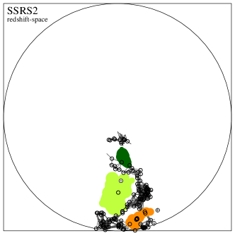
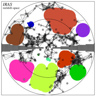
Figure 10: Voids in the SG plane: here we compare the redshift-space voids of the SSRS2 (left) and the IRAS (right). The denser sampling of the SSRS2 is evident. Similar voids are found in the overlapping regions of the surveys. For the IRAS sample compare also the real- and redshift-space distribution: the IRAS voids in redshift-space are larger, and the dense structures appear much more collapsed than in real-space (Fig. 8, panel a).

4.2 Void statistics

In order to assess the statistical significance of the voids, we have created random distributions built to mimic the geometry and density of the true sample. Averaging over the random catalogues, we derive the expected number of voids in Poisson distributions as a function of the void resolution (see Fig. 6). We will denote by $N_{\mathrm{Poisson}}(d)$ the number of voids in a Poisson distribution that contain a sphere whose diameter is $d$. The same quantity for the actual distribution will be denoted $N_{\mathit{IRAS}}(d)$. Note that $d$ scales with the selection function, correcting for the reduced density as $r$ increases. Using these void counts, we define the confidence level as

• $\displaystyle\hskip 0.0pt{p(d)=1-\frac{N_{\mathrm{Poisson}}(d)}{N_{\mathit{IRAS}}(d)}\mathrm{.}}$

The closer $p$ is to unity, the less likely such a void could appear in a random distribution. We consider voids with $p>0.95$ as statistically significant. In the IRAS sample, we have identified 12 such voids, and only these are considered in the calculations below. Our statistical confidence level should not be interpreted as the usual $2\sigma$ or $3\sigma$ grade, as the statistics we use has a different interpretation. For example, having 12 voids at a $0.95$ confidence level means that on average one finds $0.6$ such voids in the random catalogues. So, perhaps one of these 12 voids could be attributed to a random process, but we do not know which one.

Three additional voids have a moderate confidence level $0.8<p<0.95$. The fact that void 15 ($p=0.82$) is a well recognized void (the PP void) hints that all voids satisfying $p>0.8$ are worth mentioning. It is the sparseness of the IRAS 1.2-Jy that prevents us from establishing higher confidence levels: with denser surveys we expect that the physical reality of the lower confidence level voids, as well as their formal statistical confidence level, will both be established. Our experience regarding the transition to denser surveys has taught us that the new galaxies rarely appear in the voids, where most of them concentrate in the already dense areas (e.g., the extension of the CfA survey to $m_{B}\leq 15.5$ – see de Lapparent et al. 1986). Thus an IRAS extension to 0.6-Jy will probably not show smaller voids, and will enable higher statistical confidence levels. At the void resolution of $18.6h^{-1}\,\mbox{Mpc}$, $N_{\mathrm{Poisson}}(d)$ exceeds $N_{\mathit{IRAS}}(d)$, and we terminate the void search as $p$ now vanishes. At this stage, 24 voids were found in the IRAS.

In Table 2 we list the locations and properties of the fifteen $p>0.8$ voids. The 12 most significant voids ($p>0.95$) are listed in the upper part of the table. Column (1) lists the statistical confidence level $p$ of each void. The diameters given in column (2) are of a sphere with the same volume as the whole void, as is listed in column (3). The centre of the void is defined as its centre-of-(no)-mass; the distance to it, and its exact location, are given in columns (4)–(7). In column (8) we indicate the fraction of the total volume of the void covered by the single largest sphere it contains. Finally, column (9) identifies some of the voids.

The average size of the 12 significant voids in the IRAS sample as estimated from the equivalent diameters is $\bar{d}=40\pm 6h^{-1}\,\mbox{Mpc}$, consistent both with the higher $50h^{-1}\,\mbox{Mpc}$ eye estimates of Geller & Huchra [Geller & Huchra 1989] and da Costa et al. [da Costa et al. 1994], and with the lower $38h^{-1}\,\mbox{Mpc}$ estimate obtained from the first zero-crossing of the SSRS2 correlation function [Goldwirth, da Costa & van de Weygaert 1995] and from our void analysis of the SSRS2 (paper I). The increase in average void diameter in the IRAS compared to the SSRS2 ($\sim 5$ per cent) is due to the relatively narrow angular limits of the latter survey.

The 12 most significant IRAS voids occupy 22 per cent of the examined volume; considering all 24 voids, the volume is 32 per cent. If we consider only the volume-limited region of our sample, where there are no distortions caused by the $r_{\mathrm{max}}$ boundary of the survey (only by the ZOA), the void volume reaches 46 per cent. We have also examined the void distribution in redshift-space. As expected, voids in redshift-space are typically bigger than their real-space counterparts. The total void volume in redshift-space is $\sim 20$ per cent larger that that in real-space, and the average diameter of the significant voids in redshift-space is $44h^{-1}\,\mbox{Mpc}$ (compare Fig. 8, panel a, with Fig. 10, right panel).

After the voids were located we examined the locations of the previously eliminated faint galaxies. Only 204 (13 per cent) of the faint galaxies are located within the voids, in agreement with the identification of the voids based on the brighter galaxies. However, as found in the SSRS2 (paper I), there is a notable increase in the number of faint galaxies in the voids compared with the number of brighter galaxies.

What is the effect of the limitations we have imposed in our void analysis? As stated above, the treatment of the ZOA as a rigid boundary and the consideration of only empty voids cause us to interpret the results derived in this way as a lower limit. An upper limit is derived by taking the opposite approach, this time including the ZOA and filtering the field galaxies. Each factor alone corresponds to an increase in the average void diameter of 5 to 15 per cent. Together the effect is $\sim 20$ per cent, yielding an upper limit for this sample of $\bar{d}=48h^{-1}\,\mbox{Mpc}$. A similar increase occurs in the total void volume. When filtering the field galaxies the voids are not empty, now having an average underdensity of $\delta\rho/\rho\approx-0.9$, as found for the SSRS2 in paper I.

5 Discussion

Fig. 8 depicts the SG plane, as analysed using four different methods: the void finder technique, the IRAS density field [Strauss & Willick 1995] and the reconstructed velocity and density fields from the SFI sample [da Costa et al. 1996] and from the Mark III catalogue (Dekel 1994; Dekel et al., in preparation). The voids and walls identified by our algorithm indeed correspond to the under- and overdense regions in the IRAS density field respectively. Comparison with the SFI sample as well indicates a good agreement for most of the voids. On the other hand, the comparison with the Mark III map reveals several conflicts, where for instance voids 7, 11 and 15 are replaced by overdense features in the Mark III reconstruction.

Most of the overdense regions, walls and filaments are narrower than $10h^{-1}\,\mbox{Mpc}$. The smoothing scale used for creating the density fields spreads the originally thin structures over wider regions, extending into the underdense volumes. This has the effect of giving a false impression of a rather blurred galaxy distribution, where prominent overdense structures are separated by small underdense regions. The true picture is very different: there is a sharp contrast between the thin overdense structures which occupy only the lesser part of the volume, and the large voids. The notion of a void-filled universe cannot be avoided in this picture.

Comparison of panels (a) and (c) of Fig. 8 also demonstrates that the voids delineated by galaxies correspond remarkably well with the underdense regions in the reconstructed mass density field derived from peculiar velocity measurements. This supports the idea that the observed voids in redshift surveys represent true voids in the mass distribution.

An additional comparison was performed directly between two void finder reconstructions: we examined the void distribution in the region where the SSRS2 sample (paper I) overlaps the IRAS sample. Fig. 10 depicts the redshift-space voids in the SG plane, for the IRAS sample (right panel) and for the corresponding part of the SSRS2 sample (left panel). In this region we find three of the 12 significant voids identified in the SSRS2 sample. The corresponding IRAS voids are $\sim 10$ per cent larger (in diameter) than the SSRS2 ones, since they are not bounded by narrow angular limits as are the SSRS2 voids. The increase indicated here is larger than that indicated earlier (Section 4.2), where the whole surveys were compared. When only individual voids are compared, the voids in the SSRS2 located at greater distances cannot be taken into account, and these are less affected by the angular limits of the survey.

The two surveys agree not only regarding the locations of individual voids in the limited volume where the surveys overlap, but also when we compare the gross statistical properties of the voids. Both surveys show a similar void scale of $\sim 40h^{-1}\,\mbox{Mpc}$, with an average underdensity $\delta\rho/\rho\approx-0.9$. Although smaller voids could not appear in our IRAS analysis (they lack statistical significance) and larger voids could hardly fit in the volume we analyse ($r_{\mathrm{max}}=80h^{-1}\,\mbox{Mpc}$), we suggest that this void scale is indeed a characteristic physical scale.

1. Our analysis method reproduces all known voids in the regions examined, and it agrees with both the IRAS density field and the potent reconstruction based on the SFI sample.

2. A similar void scale appears in both the IRAS and the SSRS2 samples, withstanding the inherent differences between the two surveys, regarding sky coverage, galaxy selection (optical/IR) and density. Further still, the IRAS galaxies represent a special galaxy class, possibly biased relative to the optical galaxies [Lahav, Rowan-Robinson & Lynden-Bell 1988]. The two surveys agree not only statistically, but also on an individual void basis. Although the SSRS2 is much denser than the IRAS, the voids in it are not smaller.

3. An eye examination of the largest survey available today, the Las-Campanas Redshift Survey [Shectman et al. 1996] indicates again a similar void scale – the voids do not seem to be much larger although the survey is.

The characteristic void scale found in the two surveys supports the idea mentioned earlier, that the voids are also devoid of dark matter and have formed gravitationally [Piran et al. 1993].

6 Summary

We have used the void finder algorithm to derive a catalogue of voids in the IRAS redshift survey. Due to the relatively sparse sampling of this survey, we have taken a conservative approach in our analysis, looking for completely empty voids and avoiding the ZOA. As such, the average void size derived $\bar{d}=40\pm 6h^{-1}\,\mbox{Mpc}$ should be considered a lower limit for the actual size of the voids. Nevertheless, thanks to the nearly full sky coverage of the IRAS sample, it is probably the best-suited redshift survey currently available for deriving a void spectrum and for charting the nearby void cosmography. The void finder analysis clearly shows the prominence of the voids in the LSS, not hindered by smoothing of the overdense regions.

The main features of the LSS of the Universe found in the SSRS2 sample (paper I), are repeated in the IRAS sample. Namely, these are as follows.

1. Large voids occupying $\sim 50$ per cent of the volume.

2. Walls occupying less than $\sim 25$ per cent of the volume.

3. A void scale of at least $40h^{-1}\,\mbox{Mpc}$, with an average underdensity of $-0.9$.

4. Faint galaxies do not ‘fill the voids’, but they do populate them more than bright galaxies.

This consistency between IRAS and optically selected galaxies is based on an objective measurement of the most prominent feature of the LSS of the Universe, the voids, suggesting that galaxies of different types delineate equally well the observed voids. Therefore galaxy biasing is an unlikely mechanism for explaining the observed voids in redshift surveys. Comparison with the recovered mass distribution further suggests that the observed voids in the galaxy distribution correspond well to underdense regions in the mass distribution. If true this will confirm the gravitational origin of the voids.

This paper has been typeset from a TeX/LaTeX file prepared by the author.

References

- Blumenthal et al. 1992 Blumenthal G. R., da Costa L. N., Goldwirth D. S., Lecar M., Piran T., 1992, ApJ, 388, 234
- Bouchet et al. 1993 Bouchet F. R., Strauss M. A., Davis M., Fisher K. B., Yahil A., Huchra J. P., 1993, ApJ, 417, 36
- da Costa et al. 1988 da Costa L. N. et al., 1988, ApJ, 327, 544
- da Costa et al. 1994 da Costa L. N. et al., 1994, ApJ, 424, L1
- da Costa et al. 1996 da Costa L. N., Freudling W., Wegner G., Giovanelli R., Haynes M. P., Salzer J. J., 1996, ApJ, 468, L5
- de Lapparent, Geller & Huchra 1986 de Lapparent V., Geller M. J., Huchra J. P., 1986, ApJ, 302, L1
- Dekel 1994 Dekel A., 1994, ARA&A, 32, 371
- Dekel et al. 1993 Dekel A., Bertschinger E., Yahil A., Strauss M. A., Davis M., Huchra J. P., 1993, ApJ, 412, 1
- Dekel et al. 1997 Dekel A., Eldar A., Kolatt T., Yahil A., Willick J. A., Faber S. M., Corteau S., Burstein D., 1997, in preparation
- Dubinski et al. 1993 Dubinski J., da Costa L. N., Goldwirth D. S., Lecar M., Piran T., 1993, ApJ, 410, 458
- El-Ad & Piran 1997 El-Ad H., Piran T., 1997, ApJ, submitted
- El-Ad, Piran & da Costa 1996, hereafter paper I El-Ad H., Piran T., da Costa L. N., 1996, ApJ, 462, L13 (paper I)
- Fisher et al. 1995 Fisher K. B., Huchra J. P., Strauss M. A., Davis M., Yahil A., Schlegel D., 1995, ApJS, 100, 69
- Freudling, da Costa & Pellegrini 1994 Freudling W., da Costa L. N., Pellegrini P. S., 1994, MNRAS, 268, 943
- Geller & Huchra 1989 Geller M. J., Huchra J. P., 1989, Sci, 246, 897
- Goldwirth, da Costa & van de Weygaert 1995 Goldwirth D. S., da Costa L. N., van de Weygaert R., 1995, MNRAS, 275, 1185
- Kirshner et al. 1981 Kirshner R. P., Oemler A. Jr., Schechter P. L., Shectman S. A., 1981, ApJ, 248, L57
- Lahav, Rowan-Robinson & Lynden-Bell 1988 Lahav O., Rowan-Robinson M., Lynden-Bell D., 1988, MNRAS, 234, 677
- Piran et al. 1993 Piran T., Lecar M., Goldwirth D. S., da Costa L. N., Blumenthal G. R., 1993, MNRAS, 265, 681
- Shectman et al. 1996 Shectman S. A., Landy S. D., Oemler A., Tucker D. L., Lin H., Kirshner R. P., Schechter P. L., 1996, ApJS, 470, 172
- Strauss & Willick 1995 Strauss M. A., Willick J. A., 1995, Phys. Rep., 261, 271
- Tully 1987 Tully R. B., 1987, Nearby Galaxies Atlas. Cambridge Univ. Press, Cambridge
- van de Weygaert & van Kampen 1993 van de Weygaert R., van Kampen E., 1993, MNRAS, 263, 481
- Watson & Rowan-Robinson 1993 Watson J. M., Rowan-Robinson M., 1993, MNRAS, 265, 1027
- Yahil et al. 1991 Yahil A., Strauss M. A., Davis M., Huchra J. P., 1991, ApJ, 372, 380