A HIGH-RESOLUTION MAP OF THE COSMIC MICROWAVE BACKGROUND AROUND THE NORTH CELESTIAL POLE

Max Tegmark^1,2,3, Angélica de Oliveira-Costa^2,3,4, Marc. J. Devlin⁴, C. Barth Netterfield⁴, Lyman Page⁴ & E. J. Wollack⁴

¹Max-Planck-Institut für Physik, Föhringer Ring 6,D-80805 München
²Max-Planck-Institut für Astrophysik, Karl-Schwarzschild-Str. 1, D-85740 Garching; angelica@mpa-garching.mpg.de
³Institute for Advanced Study, Olden Lane, Princeton, NJ 08540; max@ias.edu
⁴Princeton University, Department of Physics, Jadwin Hall, Princeton, NJ 08544; page@pupgg.princeton.edu

1 INTRODUCTION

Since the fluctuations in the Cosmic Microwave Background (CMB) depend on a large number of cosmological parameters (see Hu, Sugiyama & Silk 1996 for a recent review), accurate CMB measurements could enable us to measure parameters such as the Hubble constant, the density parameter $\Omega$, etc. to hitherto unprecedented accuracy (Jungman et al. 1996). After the successful measurements of large-scale fluctuations by COBE team (Smoot et al. 1992; Bennett et al. 1996), attention is now shifting towards measurements at higher angular resolution.

When reducing a CMB data set, one usually wants to produce either an estimate of the angular power spectrum $C_{\l}$ or a map. Although it is the former that is ultimately used to constrain cosmological parameters, there are a number of reasons for why map making is useful as well (apart from a general desire to map the sky in as many frequency bands as possible):

• It facilitates comparison with other experiments.

• It facilitates comparison with foreground templates such as the DIRBE maps.

• It may reveal flaws in the model that are not visible in the power spectrum, such as non-Gaussian CMB features, point sources and spatially localized systematic problems.

The first degree-scale map reconstructed from difference measurements was produced by White & Bunn (1995) using data from the MAX experiment, which probed a strip of sky a few degrees wide at a resolution of half a degree. The purpose of this Letter is to present a map based on data from the Saskatoon (SK) experiment (Wollack et al. 1996; Netterfield et al. 1997, hereafter “N97”). This map covers a larger patch of sky: a cap of $15^{\circ}$ diameter centered on the North Celestial Pole (NCP). The angular resolution is similar to that of MAX (about half a degree for the SK95 data), but the region in question is more evenly sampled than was the case with the MAX map, with no “holes”.

The map-making method we employ is described in Section 2 and the results are presented and discussed in Section 3.

2 METHOD

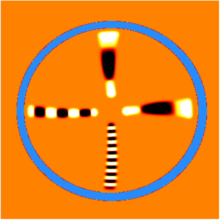
Figure 1: Sample Saskatoon weight functions.

The task of generating maps from the Saskatoon data is complicated by the fact that the data set does not contain simple sky temperatures, but rather $2590$ different linear combinations of sky temperatures. The $i^{th}$ data point, which we denote $y_{i}$, is a linear combination of the temperature across the sky, where the weights ascribed to each patch of sky are given by some known function $f_{i}(\widehat{\bf r})$. These weight functions are described in detail in N97. For illustration, four sample weight functions are shown in Figure 1. All weight functions emanate approximately radially from the NCP, oscillate in the radial direction, cover only a small RA-band, and extend to about $8^{\circ}$ from the pole. The rest of this section describes the inversion process of reconstructing a map from these linear combinations $y_{i}$.

2.1 Wiener filtering

Wiener filtering is a general method for estimating a signal from noisy data (Wiener 1949), and can be derived as follows. Suppose that we have a vector of $n$ data points ${\bf y}$ and wish to estimate a vector of $m$ numbers ${\bf x}$ (for instance the pixel temperatures in a map) from it. Without loss of generality, we can assume that both vectors have zero mean, i.e., $\langle{\bf x}\rangle=0$ and $\langle{\bf y}\rangle=0$, since otherwise, we could redefine them so that they do. Denoting the estimate of ${\bf x}$ by $\tilde{\bf x}$, the most general linear estimate can clearly be written as

$$\tilde{\bf x}\equiv{\bf W}{\bf y}$$ (1)

for some $m\times n$ matrix ${\bf W}$. Defining the error vector as $\hbox{\bfmath\char 34\relax}\equiv\tilde{\bf x}-{\bf x}$, a natural measure of the errors is the quantity $|\hbox{\bfmath\char 34\relax}|$, which is just $m$ times the r.m.s. error per data point. The expectation value of $|\hbox{\bfmath\char 34\relax}|^{2}$ is given by

$$\langle|\hbox{\bfmath\char 34\relax}|^{2}\rangle=\langle({\bf W}{\bf y}-{\bf x})^{t}({\bf W}{\bf y}-{\bf x})\rangle=\hbox{tr}\>\left[{\bf W}\langle{\bf y}{\bf y}^{t}\rangle{\bf W}^{t}-2\langle{\bf x}{\bf y}^{t}\rangle{\bf W}^{t}+\langle{\bf x}{\bf x}^{t}\rangle\right].$$ (2)

The Wiener filter ${\bf W}$ is the matrix that minimizes this error. By differentiating with respect to the components of ${\bf W}$, we obtain the simple result

$${\bf W}=\langle{\bf x}{\bf y}^{t}\rangle\langle{\bf y}{\bf y}^{t}\rangle^{-1}.$$ (3)

Direct substitution shows that the covariance matrix of the estimates is

$$\langle\tilde{\bf x}\tilde{\bf x}^{t}\rangle=\langle{\bf x}{\bf y}^{t}\rangle\langle{\bf y}{\bf y}^{t}\rangle^{-1}\langle{\bf y}{\bf x}^{t}\rangle$$ (4)

and that the error covariance matrix is

$$\langle\hbox{\bfmath\char 34\relax}\hbox{\bfmath\char 34\relax}^{t}\rangle=\langle{\bf x}{\bf x}^{t}\rangle-\langle{\bf x}{\bf y}^{t}\rangle\langle{\bf y}{\bf y}^{t}\rangle^{-1}\langle{\bf y}{\bf x}^{t}\rangle.$$ (5)

Linear filtering techniques have recently been applied to a range of cosmological problems. Rybicki & Press (1992) give a detailed discussion of the one-dimensional problem. Lahav et al. (1994), Fisher et al. (1995) and Zaroubi et al. (1995) apply Wiener filtering to galaxy surveys. The COBE DMR maps have been processed both with Wiener filtering (Bunn et al. 1994; Bunn et al. 1996) and with other linear filtering techniques (Bond 1995).

2.2 Application to the Saskatoon case

In our case, the observed data point $y_{i}$ is the true sky temperature distribution $x(\widehat{\bf r})$ convolved with the $i^{th}$ beam function $f_{i}(\widehat{\bf r})$, with noise $n_{i}$ added afterwards, so

$$y_{i}=n_{i}+\int f_{i}(\widehat{\bf r})x(\widehat{\bf r})d\Omega.$$ (6)

Our maps will cover a square region of $20^{\circ}\times 20^{\circ}$ centered on the NCP, pixelized into a $64\times 64$ square grid, so $m=4096$. To ensure that the maps are properly oversampled, we define the pixels to be the sky temperatures after Gaussian smoothing on a scale of $\sigma=1^{\circ}$:

$$x_{i}=\int\phi(\widehat{\bf r}_{i}\cdot\widehat{\bf r})x(\widehat{\bf r})d\Omega,$$ (7)

where $\widehat{\bf r}_{i}$ is a unit vector in the direction of the $i^{th}$ pixel and

$$\phi(\cos\theta)\equiv{1\over 2\pi\sigma^{2}}e^{-\theta^{2}/2\sigma^{2}}.$$ (8)

This means that the map resolution $\sigma$ is $3.2$ times the pixel separation $20^{\circ}/64$, which is safely above the Shannon oversampling rate of 2.5. In order to apply the Wiener filtering procedure, we need to compute the matrices $\langle{\bf y}{\bf y}^{t}\rangle$ and $\langle{\bf x}{\bf y}^{t}\rangle$. The former contains the correlation between the data points and themselves, and is given by

$$\langle y_{i}y_{j}\rangle=\langle n_{i}n_{j}\rangle+\int\int f_{i}(\widehat{\bf r})f_{j}(\widehat{\bf r}^{\prime})c(\widehat{\bf r}\cdot\widehat{\bf r}^{\prime})d\Omega d\Omega^{\prime},$$ (9)

where the correlation function $c$ is given by the angular power spectrum $C_{\l}$ through the familiar relation

$$c(\cos\theta)=\sum_{\l=0}^{\infty}\left({2\l+1\over 4\pi}\right)P_{\l}(\cos\theta)C_{\l},$$ (10)

where ${\bf P}_{\l}$ are the Legendre polynomials. As described in N97, the noise covariance matrix $\langle{\bf n}{\bf n}^{t}\rangle$ is almost diagonal for the Saskatoon experiment, but there are a small number of non-zero correlations (for example, there is a $2\%$ anticorrelation between the Ka94 5pt East data and the simultaneously acquired Ka94 7pt East data due to mainly to atmospheric noise).

Likewise, the correlation between the data points and the pixels is given by

$$\langle x_{i}y_{j}\rangle=\int\int\phi(\widehat{\bf r}_{i}\cdot\widehat{\bf r}^{\prime})f_{j}(\widehat{\bf r})c(\widehat{\bf r}\cdot\widehat{\bf r}^{\prime})d\Omega d\Omega^{\prime}.$$ (11)

2.3 Practical Issues

To compute the covariance matrices $\langle{\bf x}{\bf y}^{t}\rangle$ and $\langle{\bf y}{\bf y}^{t}\rangle$, we approximate the integrals in equations (9) and (11) by sums over a $256\times 265$ grid of points. Direct computation of $\langle{\bf y}{\bf y}^{t}\rangle$ with this procedure would take over a decade on a typical workstation, even if the code were optimized by omitting from the double sum all pixels where $f_{i}$ or $f_{j}$ are zero. Fortunately, the relevant angular separations are all much less the a radian, which means that the effect of sky curvature is negligible. To a good approximation, we can thus integrate over a flat two-dimensional plane instead and obtain

$$\langle{\bf y}{\bf y}^{t}\rangle-\langle{\bf n}{\bf n}^{t}\rangle\approx\int\int f_{i}({\bf r})f_{j}({\bf r}^{\prime})c({\bf r}-{\bf r}^{\prime})d^{2}rd^{2}r^{\prime}=\int\int f_{i}({\bf r})(f_{j}\star c)({\bf r})d^{2}r,$$ (12)

where $\star$ denotes convolution. Using fast Fourier transforms (FFTs) to compute the convolutions, the entire covariance matrix can now be computed in merely a day. The computation of $\langle{\bf x}{\bf y}^{t}\rangle$ can be accelerated in the same way.

Because the electronic offset is unknown, the means must be removed from the observations with each of the 64 synthesized beam patterns, which corresponds to multiplying the data vector ${\bf y}$ by a certain projection matrix ${\bf P}$. We thus use the corrected covariance matrices $\langle{\bf x}{\bf y}^{t}\rangle{\bf P}^{t}$ and ${\bf P}\langle{\bf y}{\bf y}^{t}\rangle{\bf P}^{t}$ in place of $\langle{\bf x}{\bf y}^{t}\rangle$ and $\langle{\bf y}{\bf y}^{t}\rangle$ in equation (3). We find that this correction makes a difference of only a few percent.

3 RESULTS AND CONCLUSIONS

The resulting map is shown in Figure 2 (bottom right) and in Figure 3. The fiducial power spectrum used is described in section 3.2 below. As expected, it contains virtually no features more than $8^{\circ}$ from the center, reflecting the fact that the sky outside of this circle was not probed by any of the beam functions. Computation of the relevant covariance matrices shows that the signal-to-noise ratio within this disc is fairly constant and of order two. In other words, the main features visible in this map are expected to be real rather than mere noise fluctuations. We also generated a number of mock Saskatoon data sets, ran them through the inversion software and compared the reconstructions with the original maps, which confirmed this conclusion.

3.1 Comparison between Years

The three first panels in Figure 2 show maps generated from the subsets of the data that were taken in 1993, 1994 and 1995, respectively. The 1993 data is seen to be rather featureless, reflecting the fact that the 1993 data set (42 data points) contains considerably less information than the other two years of data. Similarly, the 1995 map is seen to contain more small-scale structure than the 1994 map, reflecting the fact that the angular resolution was approximately doubled in 1995. Most potential sources of problems with the experiment (underestimation of atmospheric contamination, sidelobe pickup from celestial bodies, etc.) would be expected to vary on timescales much shorter than a year. In addition, the beam patterns were quite different in the three years as described in N97 – for instance, the beam width was substantially reduced in 1995 as mentioned above. The visual similarity between these independent maps therefore provides reassuring evidence that the bulk of the signal being detected is in fact due to temperature-fluctuations on the sky rather than unknown systematic problems.

In addition to a qualitative visual inspection, the 1994 and 1995 maps can be used to make more quantitative consistency checks. For example, we subtracted one from the other and compared the resulting noise levels with the theoretical expectations (as given by the diagonal of $W\langle{\bf n}{\bf n}^{t}\rangle W^{t})$. The levels are in good agreement, indicating that there is no evidence for additional unmodeled/overlooked sources of noise.

The perhaps most striking single feature in the maps, which stands out in all three years of data, is the large cold spot around “two o’clock”, about half way from the center. It is interesting to note that the existence of this cold spot can be qualitatively inferred from the plots of the raw data in Wollack et al. (1993) and Netterfield et al. (1994), since the three-point beam (which has a positive lobe half-way from the center) was found to give large negative temperature between 4 and 5 hours in $RA$.

3.2 Dependence on method details

To test if the reconstructed map is sensitive to the pixel size, the analysis was repeated with $32\times 32$ pixels. As expected, this produced virtually identical maps, since the original $64\times 64$ pixel map was substantially oversampled.

The maps in Figure 2 where generated using a a featureless (flat) fiducial power spectrum $C_{\l}=6Q^{2}/\l(\l+1)$ normalized to $Q=20{\rm\mu K}$. To what extent do the maps depend on this choice? As described below, the short answer to this question is “almost not at all”. As a test, we repeated the analysis for flat power spectra with $Q=0$, $10{\rm\mu K}$, $47{\rm\mu K}$ (the best fit to the Saskatoon power spectrum points of N97) and $60{\rm\mu K}$, as well as for four different normalizations of the standard CDM models (Sugiyama 1995). The spatial features remained essentially unchanged, and the different normalizations simply caused different degrees of smoothing. The appearance of the map depended essentially only on one single property of the power spectrum: the broad-band power on the angular scales where the SK experiment is sensitive. This behavior is easy to understand from equation (3). Note that whereas $\langle{\bf y}{\bf y}^{t}\rangle$ is a sum of two contributions, one from signal and one from noise, $\langle{\bf x}{\bf y}^{t}\rangle$ depends only on the signal. Roughly speaking, ${\bf W}$ is thus of the form signal/(signal+noise). In the extreme case of no signal ($Q=0$), the Wiener-filtered map thus becomes identically zero, since $\langle{\bf x}{\bf y}^{t}\rangle=0$. If we increase the assumed signal-to-noise ratio, generic components of ${\bf W}$ increase in magnitude, and the Wiener filtering process will attempt to recover more details in the map. Since the noise loosely speaking enters on smaller scales than the signal, assuming a lower signal-to-noise ratio will basically cause the filtering to suppress high frequencies more than low frequencies, i.e., smooth the map more. In summary, using a fiducial power spectrum with the wrong amount of power in the SK band will produce a map with the same spatial features in the same locations, but simply smoothed either more or less than what is optimal.

Which is the best fiducial power level to use? The answer to this question depends on our desired signal-to-noise ratio $S/N$ (which we define as the ratio of the r.m.s. signal and the r.m.s. noise). The variance in a map pixel is given by the corresponding diagonal element of $W\langle{\bf y}{\bf y}^{t}\rangle W^{t}$, so we can separate the contributions of signal and noise by splitting $\langle{\bf y}{\bf y}^{t}\rangle$ into a signal and a noise part and then compute $S/N$. Since the Wiener filtering balances between smoothing too little (getting swamped by noise) and smoothing too much (loosing unnecessarily much of the small-scale signal), it typically produces a map where these two problems are comparable in magnitude, i.e., where the noise is comparable to the lost part of the signal. Since $S/N$ compares the noise to the part of the signal which was not lost, there is no a priori guarantee that the $S/N$ obtained will be satisfactory. It is thus common to adjust the fiducial power level to obtain a desired $S/N$. In our case, $S/N\approx 1.3$ for the combined map when the fiducial band power was $Q=47{\rm\mu K}$, so we chose $Q=20{\rm\mu K}$ to get a more smoothed and less noisy map, which has $S/N\approx 2.0$.

By dividing the map by the r.m.s. noise $\sigma$, we can read off the significance level of individual map features. For instance, the cold spot around “two o’clock” is $-7\sigma$, the one at “eight o’clock” is $-5\sigma$ and the hot spot at “ten o’clock”, near the center, is $+5\sigma$.

In conclusion, we have presented the largest map to date of the CMB at degree scale angular resolution. The signal-to-noise ratio is of order two, and some individual hot and cold spots are significant at the $5\sigma$ level. It is hoped that this map can be used to make comparisons between experiments and with various foreground templates, thereby improving our understanding of systematics and foregrounds in preparation for the next generation of CMB missions.

The authors wish to thank David Wilkinson for helpful comments on the manuscript. Support for this work was provided by NASA through a Hubble Fellowship, HF-01084.01-96A, awarded by the Space Telescope Science Institute, which is operated by AURA, Inc. under NASA contract NAS5-26555, by European Union contract CHRX-CT93-0120, by Deutsche Forschungsgemeinschaft grant SFB-375, by NSF grant PH 89-21378, NASA grants NAGW-2801 and NAGW-1482, a Cottrell Scholar Award of Research Corp, a David Lucile Packard Foundation Fellowship, and an NSF NII grant to L. Page.

4 REFERENCES

Bennett, C. L. 1996, ApJ, 464, L1.

Bond, J. R. 1995, Phys. Rev. Lett., 74, 4369.

Bunn, E. F. et al. 1994, ApJ, 432, L75.

Bunn, E. F., Hoffmann, Y & Silk, J 1996, ApJ, 464, 1.

Fisher, K. B. et al. 1995, MNRAS, 272, 885.

Hu, W., Sugiyama, N. & Silk, J. 1996, preprint astro-ph/9604166.

Jungman, G.. Kamionkowski, M., Kosowsky, A & Spergel, D. N. 1996, Phys. Rev. D, 54, 1332.

Lahav, O. et al. 1994, ApJ, 423, L93.

Netterfield et al. 1995, ApJ, 445, L69.

Netterfield, C. B. et al. 1997, ApJ, 474, 47.

Rybicki, G. B. & Press, W. H. 1992, ApJ, 398, 169.

Smoot, G. F. et al. 1992, ApJ, 396, L1.

Sugiyama, N. 1995, ApJS, 100, 281.

White, M. & Bunn, E.F. 1995, ApJ, 443, L53.

Wiener, N. 1949, Extrapolation and Smoothing of Stationary Time Series (NY: Wiley).

Wollack, E. J. et al. 1993, ApJ, 419, L49.

Wollack, E. J. et al. 1996, preprint astro-ph/9601196.

Zaroubi, S. et al. 1995, ApJ, 449, 446.

Four of the 2590 Saskatoon weight functions are shown in a circle of diameter $16^{\circ}$ with the North Celestial Pole at the center. The weight functions are all for the 1995 East data, and correspond to the 3-point beam in the $RA=$0h azimuthal bin (top), the same beam in the $RA=$6h azimuthal bin (right), the 19-point beam in the $RA=$12h azimuthal bin (bottom) and the 7-point beam in the $RA=$18h azimuthal bin (left).

Tegmark, de Oliveira-Costa, Devlin, Netterfield, Page & Wollack 1996

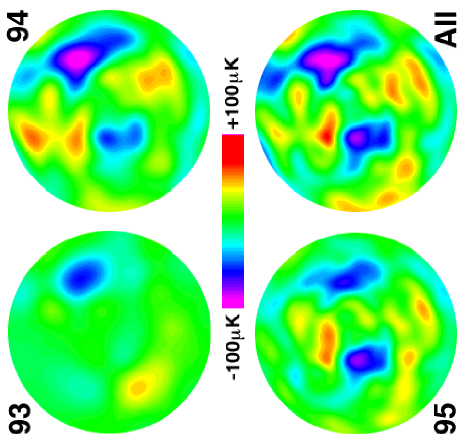
Figure 2: Wiener-filtered maps.

The CMB temperature is shown in coordinates where the North Celestial Pole is at the center of a circle of $16^{\circ}$ diameter, with $RA$ being zero at the top and increasing clockwise. The first three panels show the maps using only the 1993, 1994 and 1995 data sets, respectively. The last panel (bottom right) shows the map based on all three years of data.

Figure 3: The Wiener-filtered map.

The map based on the entire data set (bottom right in Figure 2) is shown in coordinates where the North Celestial Pole is at the center of a $20^{\circ}\times 20^{\circ}$ square with $RA$ being zero at the top and increasing clockwise. $RA=0$ is at $(x,y)=(0,10^{\circ})$. The contour curves correspond to $-75{\rm\mu K}$, $-50{\rm\mu K}$, $-25{\rm\mu K}$, $25{\rm\mu K}$, $50{\rm\mu K}$ and $75{\rm\mu K}$, respectively.