Hot HB stars in globular clusters - physical parameters and consequences for theory

Abstract

We present spectroscopic analyses of 17 faint blue stars in the globular cluster NGC 6752, using optical and UV spectrophotometric data and intermediate resolution optical spectra. Effective temperatures, surface gravities, and helium abundances of the stars are determined and compared to theoretical predictions. All stars are helium deficient by factors ranging from 3 to more than 100, indicative of gravitational settling of helium. Stars with effective temperatures above about 20000 K (sdBs) fit well to the evolutionary tracks, whereas the cooler stars show lower surface gravities than theoretically expected. This agrees with earlier findings by Moehler et al. ([1995a]) for the faint blue stars in M 15. Deriving masses from the atmospheric parameters and the cluster distance leads to a mean mass of the sdB stars of 0.50  $\rm M_{\odot}$ and a standard deviation of about 0.043 dex, which is below the value derived of the observational errors and therefore consistent with a very narrow mass distribution. The mean mass is in good agreement with the (0.49 $\pm$ 0.02)  $\rm M_{\odot}$  expected if sdB stars are extreme horizontal branch stars with a helium core of 0.48  $\rm M_{\odot}$ and an extremely thin hydrogen layer. The cooler stars however show a significantly lower mean mass of 0.30  $\rm M_{\odot}$ with a standard deviation of the mean of 0.059 dex in agreement with the findings of Moehler et al. ([1995a]) and de Boer et al. ([1995]) for the BHB stars in M 15 and NGC 6397, respectively. The problems presented by the different mass distributions of BHB and sdB stars within one cluster are discussed.

1 Introduction

The horizontal branches (HBs) in colour-magnitude diagrams (CMDs) of galactic globular clusters show a large variety in morphology: On the blue side of the RR Lyrae gap one may find HBs extending down to very faint magnitudes at the same blue colour (e.g. M 5, Buonanno et al., [1981]) while others are short and limited to the region near M_V = $\rm 0\stackrel{{\scriptstyle m}}{{.}}0$ (e.g. NGC 6397, Alcaino & Liller, [1980]). Also, some of these HBs appear to have gaps (e.g. NGC 288, Buonanno et al., [1984]; M 15, Buoanno et al. , [1985]) or, at least, are not populated in a smooth manner (e.g. NGC 6752, Buonanno et al., [1986]).

To distinguish the long and almost vertical extensions from the main body of the horizontal branch, the term “extended horizontal branch” (EHB) in contrast to “blue horizontal branch” (BHB) is used. In the field of the Milky Way the EHB stars are identified with the subdwarf B (sdB) stars, which have ${\rm T_{eff}}$ $>$ 20000 K and $\log{\rm g}$ $>$ 5 (Greenstein & Sargent, [1974]; Heber et al., [1984]; Moehler et al. [1990]; Saffer et al., [1994]).

Two basic scenarios for the origin of the sdB stars have been put forward in the literature: sdBs are assumed to have either originated as single stars, which for some reason have lost more of their hydrogen envelope by the time they arrive on the HB than most stars do, or they are the product of some kind of binary interaction (see Bailyn et al. [1992], for a detailed discussion). In the single star scenario, the sdB mass is close to 0.5  $\rm M_{\odot}$ and determined by the canonical helium core mass at the core helium flash (see Sweigart, [1994]). The importance of binary evolution is supported by the high binary frequency observed amongst the field sdB stars (Allard et al., [1994]; Theissen et al., [1994]). There are three variants of the binary scenario:

• Common envelope evolution can lead to the formation of subluminous O and B stars if Roche lobe overflow occurs during the ascend of the first (case B) or second (case C) giant branch (Iben & Tutukov [1985], [1993]; Iben [1986]; Iben & Livio [1993]). Well studied examples are HD 128220 (sdO+ FIV) and AA Dor. For case B evolution the sdB masses are somewhat smaller than the canonical 0.5  $\rm M_{\odot}$ (e.g. AA Dor, M = 0.3  $\rm M_{\odot}$, Kudritzki et al., [1982]), while for case C they are slightly larger than the canonical value (e.g. HD 128220, M $>$ 0.55 $\rm M_{\odot}$, Howarth & Heber, [1990]).

• Mengel et al. ([1976]) explored the possibility that sdB stars could evolve from binaries in which mass transfer is initiated at the tip of the giant branch, i.e. shortly before the ignition of the core helium flash, resulting in sdB masses very close to the canonical 0.5 $\rm M_{\odot}$.

• sdB stars can also result from the merger of a double helium white dwarf system (Iben & Tutukov, [1984]; Iben [1990]) with masses ranging from 0.3  $\rm M_{\odot}$ to 0.9  $\rm M_{\odot}$ and low mass stars formed preferably. Bailyn & Iben ([1989]) have explored this possibility for globular cluster sdBs and argue that a few tens of sdBs can be formed in a typical globular cluster, because binary-single star interactions increase the merger rate considerably, especially for the central regions of the cluster.

Therefore at least four scenarios for the origin of sdB stars are at hand. They can be distinguished observationally if the mass distribution of sdB stars can be determined, since the four scenarios predict quite different mass distributions: the single star and Mengel’s binary scenario (II) predict a sharp mass distribution peaked at the canonical mass of 0.5  $\rm M_{\odot}$, while binary scenarios (I) and (III) predict broader distributions peaked at masses below 0.5  $\rm M_{\odot}$. In order to find out which is the dominant sdB production channel in globular clusters, we have started to determine spectroscopic masses of blue horizontal branch stars in the globular clusters M 15 (Moehler et al., [1995a], paper I), NGC 6397 (de Boer et al.,[1995], paper II), and NGC 6752 (Heber et al., [1986] and this paper) from atmospheric parameters and the known cluster distances. The previous analyses of the BHB and EHB stars in NGC 6752, M 15 and NGC 6397 showed that

1. Three stars in NGC 6752 are bona fide EHB stars and cannot be distinguished from field sdB stars. One very blue star is a sdOB star which already evolved from the EHB.

2. The stars below the gap in M 15 are still BHB stars according to their atmospheric parameters ${\rm T_{eff}}$ and $\log{\rm g}$.

3. The BHB stars in M 15 and NGC 6397 show masses that are significantly lower than predicted by canonical theory.

NGC 6752 is up to now the only cluster where the gap seen in the CMD really separates sdB stars from BHB stars. For a long time it has also been the only cluster where sdBs have been securely identified at all. Additional sdB/sdOB candidates have been verified recently in M 15 (Durrell & Harris, [1993]; Moehler [1995]) and M 22 (Moehler et al., [1995b]).

NGC 6752 has a large population of EHB stars and is therefore very well suited for our aims. Early CMDs (e.g. Cannon, [1981]) display a pronounced gap (between V $\approx$ $\rm 16\stackrel{{\scriptstyle m}}{{.}}0$ and V $\approx$ $\rm 17\stackrel{{\scriptstyle m}}{{.}}0$) separating the EHB (V $>$ $\rm 17\stackrel{{\scriptstyle m}}{{.}}0$) from the BHB (V $<$ $\rm 16\stackrel{{\scriptstyle m}}{{.}}0$). More recent CMDs (Buonanno et al. [1986]), however, suggested that the gap is a region of the HB which is sparsely populated rather than devoid of stars. Therefore, we aim to study more bona fide EHB stars (below the gap, V $<$ $\rm 17\stackrel{{\scriptstyle m}}{{.}}0$) to determine their masses spectroscopically using the same methods as in Heber et al. ([1986]) and paper I. The second aim is to clarify the nature of the stars inside the HB gap region (i.e. $\rm 16\stackrel{{\scriptstyle m}}{{.}}0$ $<$ V $<$ $\rm 17\stackrel{{\scriptstyle m}}{{.}}0$), discovered by Buonanno et al. ([1986]). We also include two stars brighter than the HB gap because of their unusually blue colour.

2 Observations

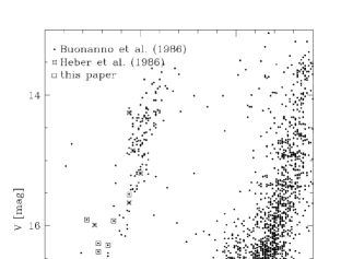
Figure 1: The colour-magnitude diagram of NGC 6752 as published by Buonanno et al. (1986). Stars analysed in this paper are marked by open squares, open stars mark the objects discussed by Heber et al. (1986). The star 3-188 of Heber et al. is not in the Buonanno data.

We selected 17 blue stars from Buonanno et al. ([1986]) for spectroscopic follow-up spectroscopy. These stars are marked in Fig. 1 with squares. Open stars in this figure mark the stars discussed by Heber et al. ([1986]). Nine stars lie below the gap in the CMD (V $>$ $\rm 17\stackrel{{\scriptstyle m}}{{.}}0$), five stars are in the gap region ($\rm 16\stackrel{{\scriptstyle m}}{{.}}0$ $<$ V $<$ $\rm 17\stackrel{{\scriptstyle m}}{{.}}0$) and three stars are above the gap (V $<$ $\rm 16\stackrel{{\scriptstyle m}}{{.}}0$), two of which have very blue colours. All optical spectra were obtained at telescopes of the ESO La Silla observatory using focal reducers. For calibration purposes we always observed 10 bias frames each night and 5-10 flat-fields with a mean exposure level of about 10000 ADU each. We obtained low resolution spectrophotometric data with large slit widths to analyse the flux distribution and medium resolution spectra to measure Balmer line profiles and helium line equivalent widths.

The atmospheric extinction was corrected using the data of Tüg (1977) and the data for the flux standard stars were taken from Hamuy et al. ([1992]).

Instrument/	Date	Telescope	CCD	pixel	no. of	gain	read-out
Mode				size	pixels		noise
				[$\mu$m]		[e-/ADU]	[e-]
EFOSC1	1992/07/04-07	3.6m	RCA # 8	15	656 $\times$ 1024	2.1	33
EMMI/B	1993/07/23-26	NTT	Tek # 31	24	1024 $\times$ 1024	3.4	5.7
EMMI/R			FA # 34	15	2048 $\times$ 2048	1.5	6.6
EFOSC2	1995/06/26-28	2.2m MPI/ESO	Th # 19	19	1024 $\times$ 1024	2.1	4.3

Instrument/	Slit	Grism/	Dispersion	Wavelength	wavelength calibration
Mode	width	Grating		range	number of	r.m.s.
					lines used	error
	[]		[Å/mm]	[Å]		[Å]
EFOSC1/low	5.0	UV300	210	3200 – 6400	11	0.5
EFOSC1/med	0.75	B150	120	3800 – 5600	12	0.3
EMMI/DIMD B	5.0	# 4	72	3400 – 5300	7	0.8
EMMI/BLMD B	1.0	# 4	72	3200 – 5100	15	0.3
EMMI/DIMD R	5.0	# 13	224	4000 – 8500	14	0.5
EFOSC2	5.0	# 1	442	1000 – 9400 (nominal)	16	1.7
				3400 – 9400 (used)

Table 1: Observation and reduction parameters

2.1 Observations in 1992

In 1992 we used EFOSC1 at the 3.6m telescope with a seeing between 1.5 and 2. Details of the setup are given in Table 1. Since the RCA chip showed some column structure we took flat-fields using U and B filters to achieve mean count levels between 5 and 10000 counts to allow a correction of the column structure. As flux standard star we observed Feige 110. During these observations the slit angle was kept at its default east-west orientation.

2.2 Observations in 1993

In 1993 we observed with EMMI at the NTT, using the two-channel mode for the low resolution spectrophotometric observations to get a longer wavelength base. Seeing values for these observations varied between 0.8and 1.5. Since no EMMI grism allows observations below 3600 Å (necessary to measure the Balmer jump) we used a grating in the blue channel and reduced the dispersion by binning along the dispersion axis by a factor of 3. For the intermediate resolution spectra we used only the blue channel and did not bin. the slit was kept at ist default east-west orientation (= 0^∘) except for the spectrophotometric observations of B 2395 (75^∘), B 4009 (75^∘), and B 4548 (85^∘). Positive angles mean anti-clockwise rotation. Since we used a narrow slit for the medium resolution observations and did not try to correct for atmospheric dispersion there are some slit losses at the blue end of the medium resolution spectra. As flux standard stars we used LTT 6248, LTT 9491, and Feige 110.

2.3 Observations in 1995

In 1995 we used EFOSC2 at the 2.2m MPI/ESO telescope to re-observe the low-resolution spectrophotometric data obtained with EMMI (see Section 3.2). Hence we only used the low resolution setup. Here we had seeing values between 1 and 1.5. Unfortunately the two nights we had were not really photometric. As we had observed the standard stars quite frequently we could however check the photometric conditions from the response curves. As flux standard stars we used EG 274 and Feige 110. During these observations we did not rotate the slit, but kept it at its default east-west orientation.

2.4 IUE data

In addition to the observations described above low resolution IUE SWP spectra are available from the archive for the stars B 491, B 916, B 4009, and B 4548. In addition to the standard reduction and calibration the correction for the new white dwarf scale as described by Bohlin et al. ([1990]) and Bohlin ([1996]) was performed. we also recalibrated the old IUE data used in Heber et al. ([1986]).

Star	X	Y	1992		1993		1995	vhel.
	[]	[]	l	m	l	m	l	[km/s]
B 210	+432	$-$389	$\times$	$\times$				$-$13
B 491∗	+344	$-$256			$\times$	$\times$	$\times$	+7
B 617	+313	$-$151	$\times$	$\times$	$\times$		$\otimes$	$-$28
B 852	+275	$-$98	$\times$			$\times$		0
B 916∗	+266	$-$296			$\times$	$\times$	$\otimes$	+12
B 1288	+212	$-$290	$\times$	$\times$	$\times$		$\times$	$-$27
B 1509	+174	+264	$\times$	$\times$		$\times$		$-$33
B 1628	+149	$-$41	$\times$			$\times$		$-$21
B 2126	+84	+383	$\times$	$\times$	$\times$			$-$25
B 2162	+76	$-$247			$\times$	$\times$	$\otimes$	$-$36
B 2395	+41	$-$277			$\times$	$\times$	$\times$	$-$52
B 3655	$-$162	+88	$\times$	$\times$	$\times$			$-$19
B 3915	$-$207	+273				$\times$		$-$9
B 3975	$-$218	$-$246			$\times$	$\times$		+18
B 4009∗	$-$222	$-$532			$\times$	$\times$		$-$56
B 4380	$-$276	$-$135	$\times$	$\times$				$-$30
B 4548∗	$-$307	+444			$\times$	$\times$	$\otimes$	$-$65

Table 2: List of observed objects. The star numbers refer to Buonanno et al. (1986). Comparing the relative coordinates given there to other photometry of NGC 6752, we found that X_B = -Y and vice versa. For stars marked with ^∗ IUE SWP are available. l (m) stands for low (medium) resolution spectra. $\times$ marks spectra observed with the respective setup, $\otimes$ marks low-resolution spectra obtained under non-photometric conditions. v_hel. is the heliocentric velocity.

3 Data Reduction

We describe the reduction of our data sets in some detail here since we encountered several problems, esp. with the spectrophotometric data, during the reduction and calibration of our observations. Since these problems on one hand affect the quality of our data (and in consequence the reliability of our analysis) and were on the other hand produced by instruments much used by observers at ESO we think that a detailed report is adequate.

3.1 EFOSC1 and EMMI data

We always averaged bias and flat-field frames for each night separately, since there were small variations in the bias frames (up to a few counts/pixel) and also a slight variation in the fringe patterns of the flat fields from one night to the next (below 5%). The dark currents were determined from several long dark frames and turned out to be negligible in all cases. To correct the electronic offset we scaled the bias frames by the mean overscan value of the science frame. To take the spectral signature out of the averaged flat field frames we fitted a 5^th (7^th) order polynomial to the blue (red) channel EMMI data. The EFOSC1 flat fields could not be fitted well enough by polynomials. We therefore averaged the mean flat-field of each night along the spatial axis, smoothed it heavily to erase all small scale structure and divided the original mean flat by the smoothed average. For the EFOSC1 data we also had to correct column structure. This correction was performed as described in paper I.

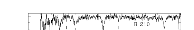
Figure 2: Normalized medium resolution EFOSC1 spectra. The part shortward of 3900 Å was normalized by taking the highest flux point as continuum value. The spectra are sorted along decreasing Balmer line depths. Small tickmarks mark steps of 20%.

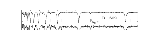
Figure 3: Normalized medium resolution EMMI spectra. The part shortward of 3900 Å was normalized by taking the highest flux point as continuum value. The spectra are sorted along decreasing Balmer line depths. Small tickmarks mark steps of 20% .

For the wavelength calibration we fitted 3^rd order polynomials to the dispersion relations. We rebinned the frames two-dimensionally to constant wavelength steps. Before the sky fit the frames were smoothed along the spatial axis to erase cosmics in the background. To determine the sky background we had to find regions without any stellar spectra, which were sometimes not close to the place of the object’s spectrum. Nevertheless the flat field correction and wavelength calibration turned out to be good enough that a linear (EFOSC1) or constant (EMMI) fit to the spatial distribution of the sky light allowed to subtract the sky background at the object’s position with sufficient accuracy. This means in our case that we do not see any absorption lines caused by the predominantly red stars of the clusters or by moon light and that the night sky emission lines in the red part could be corrected down to a level of a few percent. The fitted sky background was then subtracted from the unsmoothed frame and the spectra were extracted using Horne’s algorithm (Horne, [1986]) as implemented in MIDAS.

Finally the spectra were corrected for atmospheric extinction and response curves were derived from the spectra of the flux standard stars. Normally the response curves were fitted by a 3^rd order spline, except the red EMMI data, for which we used a 6^th order polynomial. We took special care to correctly fit the response curves for the blue low resolution data in the region of the Balmer jump, since we will use this feature for the determination of the effective temperatures of the stars.

Comparing the EFOSC1 and EMMI low resolution data for the stars observed during both runs showed that the EFOSC1 data have significantly less UV flux blueward of the Balmer jump than the EMMI data. Since both sets of spectra could be fitted with Kurucz ([1992]) models (but yielded temperatures different by up to 10000 K) we could not decide which data set was the correct one and whether one or even both data sets were hampered by instrumental effects that were not removed by the described reduction. We discussed these problems extensively with people at ESO and finally decided to repeat the spectrophotometric observations with a third instrument (which decision resulted in the 1995 observations with EFOSC2).

The medium resolution spectra observed in 1992 and 1993 are plotted in Fig. 2 and 3. Besides the Balmer lines, He I lines can easily be identified in the spectra of several of the programme stars. In addition He II, 4686 Å, is visible in B 852, which therefore has to be classified as spectral type sdOB according to the scheme of Baschek & Norris ([1975]). It is also worthwhile to note that weak Mg II, 4481 Å, absorption is detected in B 1509 and B 3975

We also used the medium resolution data to derive radial velocities, which are listed in Table 2 (corrected to heliocentric system). The error of the velocities is about 30 km/sec. Within error limits the radial velocities agree with the cluster velocity ($-$32.1 km/s, Pryor & Meylan, [1993]).

3.2 EFOSC2 data

For the EFOSC2 data we averaged the bias and flat field frames over both nights of the run, as they showed no deviations above the 1% level. The bias correction was again performed by scaling the bias with the mean overscan of the frame and we did not correct for dark current. The normalization of the flat-field was somewhat difficult: We fitted a 7^th order polynomial to the flux distribution of the averaged flat fields, which did not fit well enough the UV/blue part. We therefore averaged and smoothed the flat as described for the EFOSC1 data and merged the UV/blue part of the smoothed averaged flat and the red part of the fit at a position where the two overlapped and had a similar slope. This merged frame was smoothed again before correcting the flat.

For the wavelength calibration we again used a 3^rd order polynomial to fit the dispersion relation. However, while the wavelength calibration frames showed maximum deviations of 4 Å when rebinned using this dispersion relation, the science frames exhibited systematic shifts to the red in the order of 30 – 40 Å. The only difference between the two types of frames (beside the illumination) was the slit width, which was 1 for the calibration frames and 5 for the science frames. A possible explanation of this effect could lie with the fact that the polynomial fits normally used for wavelength calibrations are only an approximation to the true shape of the dispersion relation, which is described correctly by trigonometric functions (Strocke [1967]; Bahner [1967]). Tests performed by Rosa & Hopp (1995, priv. comm.) showed, however, that fits using such trigonometric functions are extremely unstable unless a very good guess of the true relation is already available. We therefore decided to correct the offsets by applying a mean shift of 36 Å to the blue.

Sky subtraction, correction of atmospheric extinction, and flux calibration were performed in the same way as for the EMMI and EFOSC1 data, using a constant for the spatial profile of the sky background and a spline fit for the response curve. As mentioned above we could judge the photometric quality of the observations from the response curves. We used only those curves that yielded the maximum response since those should result from observations taken without any obscurations. Several object spectra calibrated with these response curves showed an offset from the B and V magnitudes taken from Buonnano et al. ([1986]), being about 0.2 mag too faint. Although there was hardly any wavelength dependency of this offset visible we could not be sure that the absorption was truly grey. We therefore decided not to use these data for determinations of the effective temperatures because we could not rely on the continuum slope. They are marked in Table 2 by $\otimes$.

3.3 Comparison of the optical spectrophotometric data

Comparing the data for the three runs shows that the EMMI and the EFOSC2 data agree rather well when a correction for the much lower resolution of the EFOSC2 data is applied (necessary to allow comparison of the Balmer jump region). This leads to the assumption that there is some problem with the UV response of the EFOSC1 that is not corrected by flux calibration. An additional reason could lie with the extraordinarily high extinction observed at La Silla in the years 1991 and 1992 (Burki et al. [1995]). We therefore ignore all low resolution data obtained with EFOSC1 for the further analysis. As a consequence, 5 (B 210, B 852, B 1509, B 1628, B 4380) out of 17 programme stars lack reliable spectrophotometric data. For an additional star (B 3915) we do not have any low resolution data at all.

4 Atmospheric Parameters

Effective temperatures, gravities, and helium abundances are derived from line blanketed LTE model atmospheres. We used the Kurucz ([1992]) grid and models calculated with an updated version of the code of Heber ([1983]) using ATLAS6 opacity distribution functions (ODF), log(Z/ $\rm Z_{\odot}$) = $-$2.0 and helium abundance of 0.1 solar, appropriate for blue horizontal branch stars .

Kurucz ([1992]) ATLAS9 models (log g = 5.0, solar He abundance, log(Z/ $\rm Z_{\odot}$) = $-$1.5 closest to the cluster’s metallicity, [Fe/H] = $-$1.54, Djorgovski, 1993) were used to fit the energy distributions (Sect. 4.1) because of their superior spectral resolution in the region of the Balmer jump. To correct for interstellar reddening we applied the reddening law of Savage & Mathis ([1979]) and used an E_B-V of 0.05 mag.

Heber’s models were used to analyse the hydrogen and helium line spectrum (Sect. 4.2 and 4.3) in order to account for the appropriate gravities and helium abundances. As these models were computed for [M/H] = $-$2.0 (instead of $-$1.5) and sub-solar helium abundance we fitted the Kurucz hydrogen line profiles (${\rm T_{eff}}$ = 22000 K, $\log{\rm g}$ = 5.0) by Heber models of log(Z/ $\rm Z_{\odot}$) = $-$2.0. The use of different generations of ODFs (ATLAS9 versus ATLAS6) and different helium abundances turns out to be negligibly small, both for ${\rm T_{eff}}$ and $\log{\rm g}$. Hence, the following procedure is applied: The Balmer lines H_β, H_γ, and H_δ are fitted using Heber’s models. At the final parameters (${\rm T_{eff}}$, $\log{\rm g}$) curves of growths for the He I lines 4026, 4121, 4388, 4471 and 4921 Å are constructed to determine the helium abundances from equivalent widths of these lines.

In order to allow a consistent treatment of the results of Heber et al. (1986), which were obtained with solar metallicity models, we checked the effect of the metallicity on ${\rm T_{eff}}$ and $\log{\rm g}$ by fitting solar metallicity models with the [M/H] = $-$2.0 models we use now. We found out that the solar metallicity models yield effective temperatures about 1000 K lower than the metal poor models, but essentially the same $\log{\rm g}$ values. We therefore increased the ${\rm T_{eff}}$ values of Heber et al. (1986) by an offset of 1000 K to account for the lower cluster metallicity and kept the $\log{\rm g}$ values.

In the case of B 852 LTE models were found to be inappropriate due to its high ${\rm T_{eff}}$ (see Napiwotzki, [1996]). We used his NLTE models which were calculated with the code of Werner & Dreizler ([1996]) and do not include metal line blanketing. Therefore the ${\rm T_{eff}}$ scale slightly differs from the metal line blanketed scale of Kurucz and Heber models. No attempt was made for adjustment of ${\rm T_{eff}}$ scales.

Figure 4: Fits to low resolution data of B 491, B 916, and B 2395. The models are ATLAS9 (Kurucz, 1992) models of metallicity $-$1.5, all for $\log{\rm g}$ = 5.0. The asterisks mark the B and V fluxes derived from Buonanno et al. (1986) using the conversion factors given by Heber et al. (1984). The fluxes as well as the observed spectra are dereddened using the reddening law of Savage & Mathis (1979).

4.1 ${\rm T_{eff}}$ derived from energy distributions

4.1.1 IUE data and the results of Cacciari et al. (1995)

For the four stars which have IUE spectra we tried to simultaneously fit the continuum data (IUE spectra, BV photometry, continuum of the low resolution optical spectra) and the Balmer jump (cf. Fig 4). In two cases the Balmer jump suggested temperatures different from those derived from the continuum data (B 491 and B 916, cf. Table 3).

The same data have already been analysed by Cacciari et al. (1995) by calibrating UV- (1300Å -1800Å) and UV-visual (1800Å - V) colors in terms of ${\rm T_{eff}}$ and $\log{\rm g}$ using Kurucz model atmospheres. In all cases our effective temperatures are lower than the ones given by Cacciari et al. ([1995]). This can be traced back to the use of different IUE flux calibrations. We used the most recent calibration of Bohlin (1996) which gives a flux at 1800Å lower by 10% than one of the Cacciari et al. (1995) and, hence, changing the (18-V) colour by 10% , which translates in a ${\rm T_{eff}}$ decrease exactly as found when comparing our results to those of Cacciari et al.

In view of this flux calibration problem, we also went back to the IUE data for the stars analysed by Heber et al. (1986) and fitted the recalibrated IUE spectra and the optical photometric data as described above. The new temperatures were always within 1000 K of the old values and no systematic trend showed up. We therefore decided to keep the old values and only adjust them for metallicity effects (see above).

4.1.2 Optical data only

The simultaneous fitting of the spectrophotometric data (Balmer jump and continuum) and the B and V magnitudes worked well (cf. Fig. 4) in all cases except four: B 1628, B 2395, B 3655, and B 2126. B 1628 shows a strong red excess when compared to the B and V magnitudes and to the model fitting of the Balmer jump; the observed spectrum is also significantly brighter than the B and V magnitudes. The stars B 2395 (cf. Fig. 4) and B 3655 both show a moderate red excess when compared to the model fitting the Balmer jump, which also reproduces the B and V magnitudes. In the case of B 2126 the optical spectrum agrees well with BV photometry, but both show a small red excess when compared to the model fitting the Balmer jump.

Cautioned by these findings we searched all stars for red neighbours. For this purpose we used the photometry of NGC 6752 by Buonanno et al. ([1986]), and extracted for each of our targets all stars within a radius of 20(down to the limiting magnitude of about B $\approx$ $\rm 18\stackrel{{\scriptstyle m}}{{.}}5$). We then estimated the straylight provided by these stars assuming that the seeing at larger distances is best described by a Lorentz profile and scaling the intensities with the V fluxes. As seeing value we used 1.5as “intrinsic seeing” for all observations (which overestimates the seeing near the meridian) and took into account the elongation caused by atmospheric dispersion. Under these assumptions we get stray light levels of more than 3% in V for the following objects: B 617, B 1288, B 1628, B 2162, B 2395, and B 3655. As expected we found the largest values for B 1628, B 2395, and B 3655, which were observed at relatively large zenith distances and have very bright neighbours. For those objects where the neighbour did not lie in the slit the observed stray light levels are lower than the calculated ones by a factor of 1.5 to 2. The calculated excesses for B 1288 and B 617 are about 7% and cannot be measured in our spectrophotometric data. Hence we can explain the above mentioned red excesses as being caused by stray light from nearby stars (except B 2126). At the same time we can derive an upper limit of 7% for the accuracy of our spectrophotometric calibration (at V).

Since the Balmer lines (H_β, H_γ, H_δ) are diagnostic tool we also checked the stray light level in the medium resolved spectra. We used the same assumptions as above, but scaled the intensities with the B magnitudes. This results in straylight levels of at most 5% for B 617, B 1288, B 1509, B 1628, B 2162, B 2395, and B 3655. In order to estimate the effect of any additional continuum on the physical parameters we subtracted from the spectrum of B 2395 a constant offset of 5%, renormalized the spectrum and derived ${\rm T_{eff}}$ and $\log{\rm g}$ again from only fitting the Balmer line profiles. It turned out that the best fit yielded an effective temperature of 1000 K less than before and the surface gravity remained the same.

Figure 5: Fits to medium resolution data of B 491, B 916, and B 2395. The models are those of Heber (1983) for those parameters which best fitted the Balmer lines (${\rm T_{eff}}$ is already transformed to the Kurucz scale):

B 491:	${\rm T_{eff}}$ = 28000 K, $\log{\rm g}$ = 5.2
B 916:	${\rm T_{eff}}$ = 30000 K, $\log{\rm g}$ = 5.6
B 2395:	${\rm T_{eff}}$ = 22000 K, $\log{\rm g}$ = 5.0

Figure 6: Fit to medium resolution data of the sdOB star B 852. Overplotted is a Non-LTE model computed by R. Napiwotzki (priv. comm.) for a metal-free stellar atmosphere with a 0.1 solar helium abundance.

Star	V	B$-$V	${\rm T_{eff}}$,UV	${\rm T_{eff}}$,opt.	${\rm T_{eff}}$,lines	${\rm T_{eff}}$fin	$\log{\rm g}$	M	MV
	[mag]	[mag]	[K]	[K]	[K]	[K]		[ $\rm M_{\odot}$]	[mag]
Blue HB stars
B 5771	14.85	$-$0.04				13700	3.9	0.43	1.61
B 1509	15.52	$-$0.06			17000	17000	4.1	0.26	2.28
B 24541	14.27	$-$0.06				10700	3.5	0.45	1.03
B 41041	15.20	+0.00				17000	4.0	0.27	1.96
B 47191	15.65	$-$0.06				16000	4.0	0.20	2.41
Stars in the gap region
B 1628	16.30	$-$0.17			21000	21000	4.7	0.35	3.06
B 2395	16.73	$-$0.24		21000	22000	21500	5.0	0.46	3.49
B 3655	16.40	$-$0.22		24000	22000	23000	5.1	0.70	3.16
B 3975	16.27	$-$0.22		21000	21000	21000	4.8	0.46	3.03
B 4548	16.60	$-$0.14	22000	23000	23000	22500	5.2	0.75	3.36
EHB stars
B 210	17.04	$-$0.31			27000	27000	5.6	0.94	3.80
B 3311	17.12	$-$0.22				26000	5.6	0.93	3.88
B 491	17.45	$-$0.31	28000	30000	28000	28500	5.3	0.29	4.21
B 6172	17.84	$-$0.33		33000	26000	33000	6.1	0.98	4.60
B 7631	17.13	$-$0.24				27000	5.5	0.68	3.89
B 916	17.61	$-$0.26	27000	30000	30000	28500	5.4	0.32	4.37
B 1288	17.90	$-$0.31		29000	27000	28000	5.5	0.31	4.66
B 2126	17.28	$-$0.20		31000	28000	29500	5.7	0.79	4.04
B 2162	17.88	$-$0.27		35000	32000	33500	5.9	0.57	4.64
B 3915	17.16	$-$0.23			31000	31000	5.5	0.47	3.92
B 4009	17.44	$-$0.30	33000	29000	31000	31500	5.7	0.61	4.20
3-1181	17.76	$-$0.26				24500	5.2	0.23	4.52
Post-EHB stars
B 852	15.91	$-$0.28				39000	5.2	0.53	2.67
B 17541	15.99	$-$0.24				40000	5.0	0.29	2.75
B 4380	15.93	$-$0.14			32000	32000	5.3	0.93	2.69

Table 3: Physical parameters of the observed stars. The star numbers and V, B$-$V data are taken from Buonanno et al. (1986), except for 3-118, whose data were obtained from Caloi et al. (1986).
¹: Data from Heber et al. (1986), adjusted to the Kurucz temperature scale. Note that the mass value for B 1754 given by Cacciari et al. (1995) results from a incorrect bolometric correction (Cacciari, priv. comm.)
²: Since B 617 lies close to B 1288 and B 2162 in the CMD we believe that the higher temperature is the correct one (see text). It was not taken into account for the mass distribution.

4.2 Balmer line profile fits

To check the validity of the effective temperatures obtained from the low resolution data we also determined ${\rm T_{eff}}$ and $\log{\rm g}$ simultaneously by fitting the line profiles of H_β, H_γ, and H_δ.

In most cases where low and intermediate resolution spectra are available the effective temperatures derived from both agree within the error limits (cf. Fig. 5 and Table 3). In one case (B 617) however, we find an effective temperature from the low resolution data of about 33000 K, while the line profiles yield 25000 K. Since this star is in colour and brightness comparable to B 1288 and B 2162, we assume that the higher temperature is the valid one. The systematic offset between ${\rm T_{eff}}$ derived from low resolution data and from the Balmer line profiles reported in paper I could not be found with these data.

In order to get an estimate for the internal errors of the physical parameters derived from fitting the Balmer lines we used the independent line fitting code of R. Saffer (see Saffer et al., [1994]) to verify our results. It turned out that we got the same values for spectra with good S/N. For the spectra of 1992, which are considerably more noisy than the ones from 1993, we get systematically lower temperatures with Saffer’s routine than from our line profile fits (using the same set of models). Since we cannot reconcile the spectrophotometric data with the temperatures found by Saffer’s routine we decided to keep our values. The mean internal error in ${\rm T_{eff}}$ provided by Saffer’s fits are 1370 K (1992) and 460 K (1993); the mean internal error in $\log{\rm g}$ is 0.17 dex (1992) and 0.06 dex (1993).

4.3 The case of B 852

B 852 is the only star in our sample which shows He II, 4686 Å. Comparing its strength to that of He I, 4471 Å suggests a temperature exceeding 35000 K. At such high temperature deviations from LTE become important even for the relatively large gravities of hot subdwarf stars as demonstrated by Napiwotzki (1996). Therefore we used his NLTE models to derive ${\rm T_{eff}}$, $\log{\rm g}$, and helium abundance from H_β, H_γ, and H_δ, He II, 4686 Å and He I, 4471 Å, the latter line ratio being a very sensitive ${\rm T_{eff}}$ indicator. The best fit is shown in Fig. 6. The depth of the observed Balmer line profile cores cannot be reproduced by the NLTE models, which we attribute to the lack of metal line blanketing. The helium lines are not affected by this effect and are reproduced very well. We therefore use the best fit values of ${\rm T_{eff}}$ = 40000 K, $\log{\rm g}$ = 5.2 and log(n_He/n_H) = $-$2.0 as atmospheric parameters for B 852.

4.4 Final parameters

As effective temperature we finally used the mean value of all available determinations, assessing the IUE temperatures double weight because of the superior sensitivity to ${\rm T_{eff}}$ of UV data. Besides the internal errors quoted above we also have to account for systematic errors caused by the imperfections of models and data. These are estimated from the differences between various ${\rm T_{eff}}$ determinations for the same object to be about 7% in ${\rm T_{eff}}$ (cf. Table 3).

For the given final temperature we take that value of $\log{\rm g}$ as surface gravity that yields the smallest errors for the Balmer line fits at this temperature. An error in ${\rm T_{eff}}$ of 7% translates into an error in $\log{\rm g}$, which we estimated for the three groups of stars mentioned in Table 3: 0.1 dex for BHB stars ($<$${\rm T_{eff}}$$>$ = 15000 K); 0.15 dex for stars in the gap region ($<$${\rm T_{eff}}$$>$ = 22000 K) and 0.2 dex for EHB stars ($<$ ${\rm T_{eff}}$$>$ = 29000 K). Added to these errors in $\log{\rm g}$ are the internal errors given by Saffer’s fitting routine (see Sect. 4.2). For the data given by Heber et al. ([1986]) we used the mean of the errors for the 1992 and 1993 data. This results in the following errors in $\log{\rm g}$: BHB stars (1992: 0.196; 1993: 0.115); stars in the gap region (1992: 0.225; 1993: 0.160); EHB stars (1992: 0.261; 1993: 0.208). Absolute visual magnitudes were derived from the apparent magnitude and the distance modulus ((m$-$M)_V = $\rm 13\stackrel{{\scriptstyle m}}{{.}}24$, Djorgovski [1993]). Note that th reddening free distance modulus of $\rm 13\stackrel{{\scriptstyle m}}{{.}}12$ of Djorgovski agrees within the error limits with the new distance modulus (m$-$M)_V,0 = $\rm 13\stackrel{{\scriptstyle m}}{{.}}05$ derived by Renzini et al. ([1996]) by fitting the white dwarf sequence. The results are listed in Table 3.

4.5 Helium abundances

From the medium resolution spectra we could also determine the helium abundances of the stars (in case helium lines are seen) or at least upper limits. The measured equivalent widths of the He I lines are given in Table 4. Only one star (B 852) shows also He II 4686 Å. Using the physical parameters listed in Table 3 we then derive helium abundances. The spectra observed in 1992 were rather noisy and therefore equivalent widths of less than 0.35 Å cannot be measured. The data taken in 1993 are of much better quality and allow equivalent widths as low as 0.15 Å to be measured. We take these values (0.35 Å resp. 0.15 Å) as upper limits if we cannot detect a helium line in a spectrum and derive an upper limit for the helium abundance from the absence of He I, 4471 Å, the helium line predicted to be strongest in the observed wavelength range. This upper limit is determined for each object individually. All stars are helium deficient with respect to the sun by factors ranging from 3 to more than 100 and no trends with ${\rm T_{eff}}$ or $\log{\rm g}$ are apparent, similarly to the field sdBs (as demonstrated by Schulz et al., [1991]).

Name	year	4026 Å	4120 Å	4144 Å	4388 Å	4471 Å	4921 Å	log nHe	n${}_{{\rm He},\odot}/$nHe
		[Å]	[Å]	[Å]	[Å]	[Å]	[Å]
B 210	1992	0.75	-	-	-	1.06	-	$-$2.0	10
B 491	1992	-	-	-	-	-	-	$<-$3.2	$>$160
B 617	1992	-	-	-	-	-	-	$<-$2.4	25
B 8521	1993	-	-	-	-	0.26	-	$-$2.0	10
B 916	1993	0.90	0.07	0.30	-	1.40	0.40	$-$1.8	4
B 1288	1992	-	-	-	-	1.57	1.00	$-$1.5	3
B 1509	1992	0.34:	-	-	-	-	-
2	1993	0.46	-	0.12*	-	0.45	0.18*	$-$2.2	15
B 1628	1993	0.28	0.14	0.26	0.22*	0.38	0.31	$-$2.4	25
B 2126	1992	-	-	-	-	-	-	$<-$3.0	$>$100
B 2162	1993	0.49	-	-	-	0.80	0.45	$-$1.8	6
B 2395	1993	0.79	-	-	0.73	0.90	0.35	$-$1.9	7
B 3655	1992	0.80	-	-	-	0.74	0.95	$-$1.8	7
B 3915	1993	-	-	-	-	-	-	$<-$3.0	$>$100
B 39753	1993	0.73	-	0.22	0.27	0.94	0.19*	$-$2.2	15
B 4009	1993	-	-	-	-	-	-	$<-$3.1	$>$ 120
B 4380	1992	-	-	-	-	0.38:	-	$-$2.3	20
B 4548	1993	0.87	0.36:	0.97:	-	0.95	-	$-$1.9	8

Table 4: The equivalent widths of the He I lines as measured from the medium resolution spectra and the corresponding helium abundances (in particle numbers).
¹ B 852 shows also He II at 4686 Å (W_λ = 0.8 Å)
² B 1509 (1993) shows also Mg II 4481  AA (W_λ = 0.23 Å)
³ B 3975 shows also Mg II 4481 Å (W_λ = 0.26 Å) and He I 4169 Å(W_λ = 0.13: Å)
: equivalent width has a large error due to a rather noisy spectrum
$*$ equivalent width is at the level of the measuring error

4.6 Evolutionary status

The results are compared in Fig. 7 (${\rm T_{eff}}$, $\log{\rm g}$) and 8 (${\rm T_{eff}}$, M_V) to the predictions of stellar evolution theory (Dorman et al. 1993).

The bulk of the stars hotter than 20000 K lies within the theoretically predicted region (within the error bars), except three (B 852, B 1754, and B 4380). The latter three stars have about the same magnitude (V = $\rm 15\stackrel{{\scriptstyle m}}{{.}}91$–$\rm 15\stackrel{{\scriptstyle m}}{{.}}99$) and lie above the gap in the CMD, albeit far to the blue edge of the HB in this part. They are probably in a Post-EHB stage of evolution (cf. Fig. 7), as already argued by Heber et al. ([1986]) in the case of B 1754, and will evolve directly towards the white dwarf cooling sequence. The distribution of stars in the (${\rm T_{eff}}$, M_V) diagram (Fig. 8) is consistent with that in the (${\rm T_{eff}}$, $\log{\rm g}$)-plane (Fig. 7) indicating that the stars above 20000 K (except the three mentioned above) are bona fide EHB stars. The twelve stars below the gap (V $>$ $\rm 17\stackrel{{\scriptstyle m}}{{.}}0$) have a mean absolute magnitude of M_V = $\rm 4\stackrel{{\scriptstyle m}}{{.}}2$ $\pm$ $\rm 0\stackrel{{\scriptstyle m}}{{.}}3$ in excellent agreement with the mean absolute magnitude of south galactic pole sdBs, M_V = $\rm 4\stackrel{{\scriptstyle m}}{{.}}2$ $\pm$ $\rm 0\stackrel{{\scriptstyle m}}{{.}}7$ (Heber, [1986]). The five stars in the gap region ($\rm 16\stackrel{{\scriptstyle m}}{{.}}0$ $<$ V $<$ $\rm 17\stackrel{{\scriptstyle m}}{{.}}0$) have ${\rm T_{eff}}$ $>$ 20000 K, $\log{\rm g}$ near 5 and subsolar helium abundances. Therefore they show the same characteristics as the field sdB stars and have to be classified as sdBs too. However, they are somewhat more luminous (M_V = $\rm 3\stackrel{{\scriptstyle m}}{{.}}2$ $\pm$ $\rm 0\stackrel{{\scriptstyle m}}{{.}}2$) than the stars below the gap in NGC 6752 and the field sdBs.

The fact that the stars between 10000 K and 20000 K lie systematically above the HB region in the (${\rm T_{eff}}$, $\log{\rm g}$) diagram has already been noted in papers I and II and also by Crocker et al. ([1988]).

Figure 7: The resulting physical parameters listed in Table 3 compared to theoretical predictions. The solid lines are the Zero Age HB and the Terminal Age (core helium exhaustion) HB for [Fe/H] = $-$1.48 of Dorman et al. (1993). The long dashed line marks the gap region seen in the CMD by Buonanno et al. (1986). The short dashed line gives the position of the helium main sequence (Paczynski 1971). The long dashed-short dahed lines give post-EHB evolutionary tracks by Dorman et al. (1993), labeled with the total mass of the EHB star.

Figure 8: The absolute V magnitudes and effective temperatures listed in Table 3 compared to theoretical tracks by Dorman et al. (1993, details see Fig. 7). The long dashed line marks the gap region seen in the CMD by Buonanno et al. (1986).

5 Masses

Figure 9: The resulting logarithmic masses listed in Table 3 vs. $\log{\rm T_{eff}}$. The objects that were not used to derive the mean sdB mass (B 617, B 852, B 1754, B 4380) are marked by circles. Also plotted is the Zero Age HB for [Fe/H] = $-$1.48 of Dorman et al. (1993) The long dashed line marks the gap region seen in the CMD by Buonanno et al. (1986).

Knowing ${\rm T_{eff}}$, $\log{\rm g}$, and the distances of the stars we can derive the masses as described in paper I:

$\log\ (M/\mbox{\,$\rm M_{\odot}$})=const.+\log\ g+0.4\cdot((m-M)_{V}-V+V_{th})$

(V_th denotates the theoretical brightness at the stellar surface as given by Kurucz [1992].)

The results are listed in Table 3 and plotted in Fig. 9. In addition to the error in $\log{\rm g}$ errors in the absolute magnitude and the theoretical brightness at the stellar surface also enter the final error in log M. We assume an error in the absolute brightness of $\rm 0\stackrel{{\scriptstyle m}}{{.}}1$ for stars with V $\leq$ $\rm 17\stackrel{{\scriptstyle m}}{{.}}0$ and $\rm 0\stackrel{{\scriptstyle m}}{{.}}13$ for fainter stars. The error in the theoretical V brightness is dominated by the errors in ${\rm T_{eff}}$ and amounts to $\rm 0\stackrel{{\scriptstyle m}}{{.}}12$ (BHB stars); $\rm 0\stackrel{{\scriptstyle m}}{{.}}13$ (stars in the gap region); and $\rm 0\stackrel{{\scriptstyle m}}{{.}}14$ (EHB stars). Alltogether this leads to the following errors in log M: BHB stars (1992: 0.210; 1993: 0.137); stars in the gap region (1992: 0.238; 1993: 0.178); EHB stars (1992: 0.275; 1993: 0.225). To determine the mean mass of the sdBs (this paper and Heber et al., [1986]) we took all stars with ${\rm T_{eff}}$ $>$ 20000 K, excluding B 617 (due to the strange offset between temperatures from continuum and from line profiles) and the post-EHB stars B 852, B 1754, B 4380, resulting in a total of 16 stars. We then calculated the weighted mean of the logarithmic masses for these stars (the weights being derived from the inverse errors). The mean logarithmic mass for these stars then is -0.300 (= 0.500  $\rm M_{\odot}$). The logarithmic standard deviation is 0.043 dex and the expected mean logarithmic error as derived from the observational errors is 0.054 dex. The mean mass therefore agrees extremely well with the value of 0.488  $\rm M_{\odot}$ predicted by canonical HB theory for these stars (Dorman et al., 1993) and the standard deviation is less than expected. If we omit the stars observed in 1992 (due to their higher errors) we get a mean logarithmic mass for the remaining 12 stars of -0.327 (= 0.47  $\rm M_{\odot}$), which is somewhat lower than the result above but still in very good agreement with theoretical predictions. There is no significant difference between the mean mass for the eleven stars below the gap ($<$log M$>$ = -0.306; $<$M$>$ = 0.494  $\rm M_{\odot}$) and the five stars inside the gap region ($<$log M$>$ = -0.289; $<$M$>$ = 0.514  $\rm M_{\odot}$); again pointing towards their nature being identical. The five stars above the gap (V $<$ $\rm 16\stackrel{{\scriptstyle m}}{{.}}0$, ${\rm T_{eff}}$ $<$ 20000 K) have a mean logarithmic mass of $-$0.518 (= 0.303  $\rm M_{\odot}$) with a logarithmic standard deviation of 0.059 (compared to an expected error of 0.073). Canonical theory would predict for these stars a mean logarithmic mass of $-$0.256 (= 0.554  $\rm M_{\odot}$) with a scatter of 0.018 dex.

6 Conclusions

Combining our results with those of Heber et al. ([1986]) we have carried out spectroscopic analyses of 25 blue stars in NGC 6752. We studied stars both brighter and fainter then the gap region ($\rm 16\stackrel{{\scriptstyle m}}{{.}}0$ $<$ V $<$ $\rm 17\stackrel{{\scriptstyle m}}{{.}}0$) and also five stars within this gap region. The results can be summarized as follows:

• All stars are helium deficient and no trends of the helium abundance with atmospheric parameters become apparent.

• All stars below the gap (except three) lie on or close to the Horizontal Branch. The latter three stars have already evolved off the EHB towards the white dwarf cooling sequence.

• The stars fainter than the gap (V $>$ $\rm 17\stackrel{{\scriptstyle m}}{{.}}0$) are very similar to the field population of sdB stars. Their mean mass is consistent with the canonical value of half a solar mass.

• The stars inside the gap region ($\rm 16\stackrel{{\scriptstyle m}}{{.}}0$ $<$ V $<$ $\rm 17\stackrel{{\scriptstyle m}}{{.}}0$) are sdB stars too, although more luminous by one magnitude than the average field sdBs. Their mean mass is also consistent with the canonical mass. Their position in the (${\rm T_{eff}}$, $\log{\rm g}$)-plane agrees less well with HB evolutionary calculations of Dorman et al. (1993) than the fainter EHB stars do.

• The stars brighter than the HB gap have significantly lower gravities than predicted by theory. Their masses are also significantly lower than predicted by evolutionary calculations.

• The standard deviations of the mean logarithmic masses for all groups of stars are lower than expected from the observational errors.

From these results we conclude:

• The helium deficiency found in all stars is indicative for diffusion, i.e. gravitational settling of helium as is the case for the field sdB and BHB stars.

• The increased sample size allowed a more meaningfull determination of the mean mass of the sdB stars than pevious work did and it turned out to be in good agreement with the value predicted by classical EHB theory. In addition, the standard deviation is smaller than the mean error derived from the observational errors. We take this as a verification that sdB stars indeed show a very narrow mass distribution, which is in full agreement with their status as extreme HB stars with a very thin hydrogen layer, produced by the same processes that produce BHB stars. This finding, however, does not explain the gap that separates BHB from sdB stars in NGC 6752 (and also in M 15, Durrell & Harris [1993]). The mean mass and the width of the mass distribution is consistent with the single star evolutionary scenario or the Mengel et al. binary evolution scenario (No. II in the introduction) for the origin of EHB stars, but can hardly be explained within the framework of the binary scenario (I) and the merger scenario (III) listed in the introduction, since both scenarios would predict a broader mass distribution with a mean mass below 0.5  $\rm M_{\odot}$.

• The low masses as well as the low surface gravities we find for the BHB stars (brighter than the gap) remain a puzzle. Lower than expected gravities for BHB stars were also found recently by Dixon et al. ([1996]) in the globular cluster NGC 1904. Figure 10 illustrates this phenomenon with data for the globular clusters M 5, M 15, M 92, NGC 6397 and NGC 288 in addition to the data of this paper. As can be seen there the mass distribution of the BHB stars differs considerably from those of the sdB stars analysed here. The fact that the mean masses of BHB stars in globular clusters are significantly and systematically too low has already been noted in papers I and II. Most of the possible explanations of this finding (see papers I and II), however, are ruled out by the mass distribution of the sdB stars presented here: Non-solar helium abundances, peculiar metallicities due to diffusion, helium stratification, systematic errors in $\log{\rm g}$ and/or distance moduli should affect the sdB stars in the same way as the BHB stars.

• Further insight into the nature of BHB and EHB stars may come from their radial distribution. We therefore investigated the radial distribution of all stars in Buonanno et al. ([1986]) that are fainter than V = $\rm 13\stackrel{{\scriptstyle m}}{{.}}4$ and bluer than B$-$V = $\rm-0\stackrel{{\scriptstyle m}}{{.}}2$. This sample, consisting of 214 stars, was divided into two groups: BHB stars with V $<$ 16 (142), and EHB stars with V $\geq$ 16 (70), which combines all sdB stars. We then counted the stars in radial bins of 50 and normalized the numbers to the total numbers of stars in each group as well as to the area covered by each bin. The resulting radial distributions show no significant difference, supporting a similar evolutionary history and mass distribution, in contrast to the situation described above.

While the idea that there is something wrong with the model atmospheres, leading to too low values of $\log{\rm g}$ for the temperature range between 10000 K and 20000 K sounds rather intriguing and would also explain the loci of the BHB stars in the $\log{\rm T_{eff}}$-$\log{\rm g}$-diagram (cf. Fig. 9 of Paper I), it could not explain the findings of Paper II, where the physical parameters of the stars fit very well to theoretical expectations, but result nevertheless in too low masses. The remaining possibility, i.e. that the BHB masses are indeed that low puts severe problems to stellar evolutionary models, since up to now no scenario is known to produce stars in that temperature range with masses of about 0.3  $\rm M_{\odot}$.

Figure 10: The resulting masses plotted in Fig. 9 compared to masses of BHB stars in other cluster. The BHB data are taken from Paper I (M 15), II (NGC 6397), and Crocker et al. (1988, M 5, M 92, and NGC 288)