The Ellipticity and Orientation of Clusters of Galaxies in N-Body Experiments

Abstract

In this study we use simulations of 128³ particles to study the ellipticity and orientation of clusters of galaxies in N-body simulations of differing power-law initial spectra ($P(k)\propto k^{n},n=+1,0,-1,-2$), and density parameters ($\Omega_{0}=0.2$ to 1.0), in a controlled way, based on nearly 3000 simulated clusters. Furthermore, unlike most theoretical studies we mimic most observers by removing all particles which lie at distances greater than $2{\rm h^{-1}}$ Mpc from the cluster center of mass.

We computed the axial ratio and the principal axes using the inertia tensor of each cluster. The mean ellipticity of clusters increases strongly with increasing $n$. We also find that clusters tend to become more spherical at smaller radii.

We compared the orientation of a cluster to the orientation of neighboring clusters as a function of distance (correlation). In addition, we considered whether a cluster’s major axis tends to lie along the line connecting it to a neighboring cluster, as a function of distance (alignment). Both alignments and correlations were computed in three dimensions and in projection to mimic observational surveys. Our results show that significant alignments exist for all spectra at small separations ($D<15{\rm h^{-1}}$ Mpc) but drops off at larger distance in a strongly $n-$dependent way. Therefore the most useful study for observers is the variation of alignment with distance. Correlations exist but are a weaker effect.

We found that differences in $\Omega$ had no measurable effect on mean ellipticity, and a weak effect on cluster alignments and correlations. Biasing was able to totally hide the effect of greater nonlinearity. Therefore, we suggest that any effort to probe $\Omega$ in this manner be abandoned unless it can be unambiguously proven to exist on smaller scales. However, there are systematic effects due to the primordial spectral index, $n$. Our results suggest that cluster ellipticity and the scale dependence of cluster alignments probe the primordial power spectrum independently of the parameters of the background cosmology. Future work should concentrate on these parameters.

Submitted to The Astrophysical Journal LINN, ET AL. CLUSTERS OF GALAXIES IN N-BODY EXPERIMENTS

1 Introduction

A common theoretical picture of large-scale structure formation holds that a hierarchical (bottom-up) scenario will result in galaxy clusters of lower ellipticity and possessing little evidence of preferred orientation with neighbors. Alternatively, if pancake structures exist as predicted by Zel’dovich (1970), then a top-down emergence of structure should result in elliptical clusters with statistically significant alignment correlations with neighbors. Recently, these theoretical models have been effectively combined, implying a transition based on spectrum should be present (e.g. Melott and Shandarin, 1993; Pauls and Melott 1995; Bond et al. 1996). It is supposed that a model which is characterized by high power in the short-wavelength end of the spectrum should be expected to exhibit more hierarchical traits compared to a long-wavelength dominated model and its more top-down mediated structure. Furthermore, in a low density universe structure formation slows near a redshift $z\sim 1/\Omega$. Thus the cluster may undergo a long period of relaxation without additional infall after its initial formation, and may become more spherical. For these reasons, many have hoped that clusters, although nonlinear objects, may probe initial conditions. They are at the borderline of scales where hydrodynamics are thought to be essential (Summers et al. 1995).

Carter & Metcalfe (1980) showed that the distribution of galaxies within a cluster is usually not spherical,but highly elongated. Additionally, a number of studies (Rood, et al 1972, Gregory & Tifft 1976, and Dressler 1981) showed that the elongation was not due to rotation. Binggeli (1982), through his study of Abell clusters form the Palomar Sky Survey, found evidence that galaxies separated by less than $\sim 30$ Mpc exhibit a strong tendency to point at one another (we call this “alignment” hereafter). He also found that the orientation of a cluster was dependent upon the distribution of the surrounding clusters, thus arguing for an anisotropic distribution of clusters on a scale of $\sim 100$ Mpc. However, in a repeat and extension of Binggeli’s methods, Struble and Peebles (1985) found little evidence for large-scale alignment of clusters of galaxies. West (1989b) on the other hand confirmed the Binggeli result.

In more recent work, de Theije, et al (1995) (hereafter TKK) in their study of 99 low- redshift Abell clusters found that the distribution of cluster ellipticities had a peak near $e\sim 0.4$ with a maximum of $e\sim 0.8$. Rhee, et al (1992) found evidence for large-scale alignment in a study of 107 rich clusters from the Palomar Sky survey. West and colleagues have also found significant evidence to support this viewpoint. West, et al (1995) found a marked anisotropy based upon their studies of the X-ray distribution of substructure in clusters of galaxies from the Einstein observatory. In 1989, West generated a catalog of 48 superclusters based upon a large number of Abell clusters to study the shapes and orientations of those clusters. He found that the axial ratios tended to fall around 3:1:1 or 4:2:1. Furthermore, he presented evidence that on scales of as large as $\sim 60{\rm h^{-1}}$ Mpc there is a strong tendency for them to be aligned. There has thus developed over the last few years a picture in which clusters are clearly elliptical and exhibit statistically significant alignments toward other members of the parent supercluster. Recently Plionis (1994) has completed the largest up to date study of cluster alignments. He finds nearest neighbor alignments up to scales of 15 $h^{-1}$ Mpc at the 2-3 sigma significance level, while weaker alignments are detected on scales up to 60 $h^{-1}$ Mpc. Since his cluster sample is not volume limited nor redshift complete the alignments he detects are likely to reflect a real effect.

Using N-body studies of a CDM universe, West, et al (1991) (hereafter WVD) found that on scales of order $10-15{\rm h^{-1}}$ Mpc the principal axes of neighboring clusters were clearly aligned. When the sample of clusters is limited to those clusters “within a supercluster”, the alignments extend to distances as large as $\sim 30{\rm h^{-1}}$ Mpc. TKK found evidence, based upon numerical simulations of $\Omega=0.2$ CDM models, that clusters tended to be more spherical in low-omega models. This confirmed the theoretical work of van Haarlem and van de Weygaert (1993) who came to the same conclusion based upon N-body simulations of a CDM universe. Van Haarlem and Van de Weygaert also found that their simulation results are consistent with a picture in which alignments arise from the infall of substructure along a filament, anticipating a finding of West, et al (1995). Earlier, Shandarin and Klypin (1984) had explicitly interpreted the results of their simulations as showing that clusters were the result of flows along filamentary structures.

We are trying here to systematize and probe the significance of the N-body studies. In some studies, cluster separations were so large relative to the simulation volume that boundary conditions are clearly a problem. In other cases, the quantities studied,such as alignment in three dimensions are clearly not measurable in real data given the precision of non–redshift distance measures and distortions due to peculiar velocity (e.g. Praton and Schneider 1994). In studying popular scenarios, there is a tendency to vary multiple parameters at once. For example, TKK and van Haarlem and van de Weyaert (1993) simultaneously varied $\Omega_{0}$, the bias factor, and the initial power spectrum, since the low $\Omega$ CDM universe has a different transfer function and presumed bias.

Given the variety of possible theories, it is important to know what parameters are being probed and what are not, rather than relying on case–by–case checks of agreement. Ultimately, it will be necessary to do simulations large enough to sample long–wave power but able to resolve hydrodynamic scales. At that time there can be a physical basis for assuming some bias between mass and galaxies. Since dissipation erases information, our study will set an upper limit on the kind of information that can be recovered in global cluster studies. This study will clarify what can and cannot be probed by such cluster statistics.

2 N-Body Simulations

The N-body simulations used were generated using a Particle-Mesh (PM) code using a staggered–mesh scheme Melott (1986). Our simulations consisted of $128^{3}$ particles on a comoving $128^{3}$ grid (for details see Melott and Shandarin 1993). To perform the data analysis we considered only a $64^{3}$ subset of the original $128^{3}$ particles but we have checked a sample of our results for consistency with a full count. Even for our smallest clusters there was no significant difference in our main diagnostics between the subset and the use of all particles from the simulation. We ran simulations for four power law spectra, $n=1,0,-1,-2$, in both high- and low-$\Omega$ universes. Four realizations of each of the eight above initial conditions were performed. These realizations were then studied at two different evolutionary timesteps, $k_{n\ell}=8k_{f}$ and $k_{n\ell}=4k_{f}$, where the non-linear wavenumber; $k_{nl}$ is defined by

$$\sigma^{2}=a^{2}\int^{k_{nl}}_{0}P(k)d^{3}k=1,$$ (1)

where $P(k)$ is the initial power spectrum of the density fluctuations, and $a$ is the cosmic expansion factor.

In the high-$\Omega$ case, $\Omega_{0}=1$ for all cases. For the low-$\Omega$ simulations, $\Omega_{0}=0.2$ for all power laws at $k_{n\ell}=4k_{f}$ at the earlier stage $k_{n\ell}=8k_{f}$, $\Omega$ had the values $0.707,0.609,0.487$ and $0.347$ for $n=1,0,-1,$ and $-2$, respectively, and $k_{f}$ is the wavenumber of the fundamental.

Power–law spectra are not realizations of any particular scenario, but are extremely useful as probes of the physics of clustering. Since the initial spectrum is featureless, we can scale from the correlation length of mass as set to $\sim 5h^{-1}$ Mpc, setting the free “bias” parameter $b=1$. Our goal here is to find out what statistics can be useful discriminators of cosmological models.

From each realization, clusters were identified using a “friends-of-friends” technique. Any points closer than the linking distance to a given point were considered linked. The linked points were then in turn checked for points linked to them, thereby creating clusters. A linking distance of $l=0.5$ grid cells was chosen because it leads to clusters of approximately the same mass as an Abell cluster $\sim 10^{15}{\rm M_{\odot}}$ assuming $\Omega=1$. Table 1 contains the resulting box sizes for each of the models being considered here. For stage $k_{n\ell}=4k_{f}$, the ten largest clusters were selected for examination, ten being about the number of clusters expected in that volume of space (Batuski et al. 1987). In addition Hoessel et al (1980) found the observed number density of clusters of richness class $R\leq 1$ to be $n\approx 6\times 10^{-6}h^{3}{\rm Mpc^{-3}}$. Bahcall (1988) argued a more reasonable value when galactic obscuration is taken account is $n\approx 10^{-5}h^{3}{\rm Mpc^{-3}}$. Given the sizes of the computational volume given in Table 1, which are typically $\sim 100h^{-1}$ Mpc on a side, our use of 10 clusters per simulation is justified. Since stage $k_{n\ell}=8k_{f}$ represents a volume of space $2^{3}$ times greater than $k_{n\ell}=4k_{f}$, we chose eight times as many clusters (the eighty largest clusters) from each realization in that stage. In all then, our study contains 2880 clusters, many more than any previous study. None have less than 40 simulated particles, and most have many more.

We wish to stress that in this study we are restricting our attention to a controlled and systematic study of the properties of collisionless systems, i.e. dark matter, presuming that it consists of a population of weakly interacting particles. It has been shown (Suisalu and Saar 1996) that unless the comoving softening length is approximately equal to the mean interparticle distance, spurious gravitational collisions occur which scatter the particles off one another (as opposed to the mean field). In this limit a PM code is much faster than anything else.

We will thus be unable to probe the inner parts of clusters; our resolution is limited to an equivalent 0.5 Mpc in this series. However, in order to model these inner regions correctly, we would need to include hydrodynamics (e.g. Evrard et al. 1993, Summers et al 1995). By forgoing this for now, we are able to conduct a large, controlled, systematic study of the overall shapes of clusters free of two–body relaxation, as implicit in PM codes (e.g. Peebles et al. 1989).

3 Average Ellipticity

3.1 Method of Computing Ellipticity

The clusters as we find them may have arbitrary shapes, including the filaments that connect them and outliers just in the process of merging. For this reason, we follow most observers’ practice, and inscribe a sphere of radius 2.0$h^{-1}$ Mpc in radius, centered on the center of mass of the cluster. This choice is motivated by distance scales which can be separated observationally, (cf. Bahcall & Cen 1993, Rhee, et al 1991a, Rhee, et al 1991b, Rhee & Latour 1991, Binggeli 1982 ) but is nonetheless somewhat arbitrary. In computing ellipticity and orientation we use only this portion of the cluster, as in previous observational studies of this type.

The ellipticity of a cluster was found using second moments of the cluster mass. This method is similar to that outlined in TKK and Plionis, Barrow & Frenk (1991). With respect to the center of mass, the tensor for the two dimensional case is defined as

$$I_{ij}=\Sigma\chi_{i}\chi_{j}m\hskip 36.135pt(i,j,=1,2)$$

where the sum is over all points, $\chi_{1}=x$ and $\chi_{2}=y\;.$ This tensor has the same eigenvectors as the standard inertia tensor but its eigenvalues are related to axis length. For a uniform ellipsoid the ratio of eigenvalues is the square of the ratio of axes. In our simulations, the points were all of equal mass, so $m$ was set to 1. This can be easily extended to three dimensions by letting ($i,j=1,2,3$), where $\chi_{3}=z.$ $I_{ij}$ was diagonalized to find the eigenvalues and eigenvectors. The eigenvalues $\Lambda_{1},\;\Lambda_{2},\;\Lambda_{3}$ were sorted so that $\Lambda_{1}\geq\Lambda_{2}\geq\Lambda_{3}$ (or just $\Lambda_{1}\geq\Lambda_{2},$ for two dimensions). For the two dimensional case, the axial ratio was defined as

$$e=\sqrt{\Lambda_{2}/\Lambda_{1}}$$

For the three dimensional case, two axial ratios were found:

$$e_{2}=\sqrt{\Lambda_{2}/\Lambda_{1}}\;\;,\;\;e_{3}=\sqrt{\Lambda_{3}/\Lambda_{1}}$$

In order to compare our results with those of TKK, the ellipticity was defined for the two dimensional case as

$$\epsilon=1-\Lambda_{2}/\Lambda_{1}\equiv 1-e^{2}$$

The results in the 2-D case are those for projections of clusters. Because the individual clusters are oriented (as we confirmed) randomly with respect to the $x$, $y$, and $z$ axes, just as physical clusters are oriented randomly with respect to the plane of the sky, this assures an unbiased data set. For the two dimensional case, each cluster was projected onto the $xy$ and $yz$, planes, since only two projections are independent in $e$.

3.2 Average Ellipticity and Initial Conditions

In Figure 1a and 1b we plot $e_{2}$ and $e_{3}$. In Figure 1c we plot $e$ for the 2D projections. The error bars are the standard deviation of the mean value for each of the realizations. The single error bar in the lower left corner represents the dispersion in ellipticity for a typical cluster. We are probing whether systematic differences in the average values can give cosmological information, given datasets the size of our simulation volumes. Further fine tuning of observables will require imitating particular survey characteristics, which is outside the purpose of this paper. However, we can already make a number of unambiguous statements:

(a) Clusters are not spherical; in general they are triaxial.

(b) We can check for consistency by examining results in the scale–free $\Omega_{0}=1$ case. There are low–significance differences between the stages for $n=1$ in the axial ratio, smaller for smaller $n$. We have confirmed that these reflect resolution effects in our code, which affect the earlier stage $k_{n\ell}=8k_{f}$. The difference is a measure of how much numerical effects limit the precision of our answers. The change in error bars is due to a change in the sample size. At this point one might be worried that the $n$-dependent trend might be simply a numerical artifact. We have tested for this by computing the ellipticities at a later stage ($k_{nl}=4k_{f}$) of evolution where resolution is not problem. These results are also shown in figures 1a, 1b, & 1c. At this later stage the trends remain thus they cannot be due to limited dynamical range in the simulation.

(c) There is no significant difference in ellipticity between low and high $\Omega$. This appears to contradict the results of TKK and others, but we believe we understand the reasons, as explained below.

(d) There is a systematic trend with spectral index: large $n$ implies more anisotropic clusters. Thus, although it is hopeless to probe $\Omega_{0}$ with cluster ellipticities, it may possibly probe $n$ more clearly.

(e) The dispersion in ellipticity of clusters is large within a cosmological model, and large within a sample. At least 100 clusters will be needed to establish the result with sufficient precision.

(f) Clusters are more isotropic at smaller radii. (Figure 2)

Now, we compare those conclusions with other studies. (a) and (f) agree with all others where they were checked. (b) is a consistency test not performed elsewhere.

Conclusion (c) appears to conflict with TKK, as well as Evrard et al. (1993). These authors studied Cold Dark Matter models and concluded their low $\Omega_{0}$ CDM models produced much less elongated clusters. There are numerous differences with our work, including many fewer clusters, smaller total volumes studied, constrained realizations of random fields, varying size of clusters, not choosing to excise the central region of the cluster, etc. However, one consistent difference is the choice of biasing. In all these studies a bias factor $b$ (usually 1.7-2) is used with the $\Omega_{0}=1$ models. (A typographical error in TKK was confirmed in conversation with Katgert.) $b$ is typically defined as the $1/\sigma_{8}$, where $\sigma_{8}$ is the RMS mass density fluctuation in a 8 Mpc sphere. In all cases, these CDM studies have a different ratio of cluster mass to mass scale of nonlinearity for low and high $\Omega_{0}$. Further support for this point of view can be found by comparison with West et al. (1989) (hereafter WDO) who (similarly to us) found no difference between their $n=0$ low $\Omega_{0}$ and high $\Omega_{0}$ (unbiased) models.

Also, when TKK went from high to low $\Omega_{0}$ they used the CDM transfer function for each case. Low $\Omega_{0}$ CDM has a more steeply negative initial power spectrum at cluster scales than high $\Omega_{0}$. Our observed trend (d) would explain the TKK result: the change in ellipticity is a result of a different initial power spectrum, not the value of $\Omega$. Their result is true for these particular CDM alternatives, but does not generalize.

Evrard et al. (1993) examined contours at a much smaller radii than we did, so the results cannot be directly compared. The difference they found (more spherical inner contours in low $\Omega$) could be due either to the improved modeling due to including hydrodynamics, or to spurious scattering and two–body relaxation (as Suisalu and Saar 1996 found in $P^{3}M$ codes; see also Merritt 1996), or is simply a phenomenon of small radii only.

Conclusion (d) does not appear in the conclusions of West et al, 1989, hereafter WDO and Efstathiou et al. (1988), who found no significant trend in ellipticity with power–law index. However, WDO had too few clusters (20 per spectral type) to see these trends. Our results are consistent with theirs. In Figure 1 the standard deviation for one cluster, shown as the single error bar in the lower left corner, (rather than the mean in the volume) is about an order of magnitude larger. It is clear that large ensembles such as those to come from the Sloan Sky Survey are needed to measure these effects. On the other hand, Efstathiou et al. (1988) who had enough objects to see this made a fatal cut: they excluded from consideration as clusters any $n$–body clumps which were not “smooth”, i.e. had no central mass condensations as measured by asymmetry at a variety of radii. Since the asymmetries are typically generated by mergers falling in along bridges that connect clusters (Shandarin and Klypin 1984, TKK) cutting out these “unsmooth” clumps means eliminating the main source of anisotropy. Most real clusters are not smooth. X-imaging results from the Einstein satellite first revealed the complexity of the intracluster medium (Forman, et al 1981; Henry et al. 1981). Since then both optical (Geller & Beers 1982; Baier 1983; Beers, et al. 1991; Bird 1993, 1994a,b) and X-ray (Jones & Forman 1992; Davis & Mushotzky 1993; Mohr, et al. 1993) studies have continued to support the presence of significant substructure in galaxy clusters (for a theoretical perspective see Dutta 1995; Crone, et al. 1995; Splinter & Melott 1996). These results contradict many early studies in which smooth configurations were assumed (cf. Kent & Gunn 1982; Kent & Sargent 1983). Thus, Efstathiou et al (1988) eliminated the most interesting cases.

The trend we observe, that of increasing ellipticity with increasing $n$, can be understood by considering the mass function (Press and Schechter 1974). For larger $n$, the mass function dives down more steeply at small masses. Thus, for large $n$, mergers are more often between large clumps, which significantly perturbs the shape. For smaller $n$, the clusters grow by accretion of smaller clumps, tending toward accretion of homogeneous mass as $n$ approaches -3. Accretion of many small clumps tends to leave the cluster shape undisturbed, as seen in our results.

We confirm (Figures 2a,2b & 2c) that clusters become more isotropic in their shape at smaller radii. The figure also compares (for spectral index $n=-1$) an $\Omega=1$, $b=1$ simulation and a low $\Omega$, $b=1$ simulation. This bias is defined operationally by comparing the 10 largest clusters in a $k_{n\ell}=4k_{f}$ box with the 10 largest clusters in a $k_{n\ell}=8k_{f}$ box (which would be taken to contain 80 clusters if $b=1$). We find essentially identical runs of ellipticity with radius, suggesting they cannot be distinguished by this procedure. Biasing appears able to imitate the effect of more nonlinearity for cluster ellipticity.

4 Alignments & Correlations

4.1 Alignment

We use alignment of a cluster to refer to whether the principal axis points along the line joining it to a neighboring cluster. This continues investigation into suggestions of Tifft (1980) and Binggeli (1982). The principal axis is determined from the eigenvectors of the inertia tensor, found above. The eigenvector associated with the largest eigenvalue is the longest principal axis of the cluster.

The cosine of the angle $\alpha$ between a cluster’s longest principal axis and the line connecting it to a neighboring cluster was plotted against the distance between the two clusters. In order to remove effects of boundary conditions, the cluster–cluster distance was never larger than $L/4$.

We attempted to quantify this observation in three ways. We determined the mean and standard deviation of $cos\;\alpha$ using all the data points. $<cos\alpha>$ is 0.5 for a random uniform three dimensional distribution, and $<\alpha>$ is $45^{\odot}$ for a random two dimensional distribution. We also examined projected angles, since the full angle is not observable.

4.2 Correlation

We use here “correlation” of two clusters as a measure of whether their longest principal axes point in the same direction. This would be likely if ellipticities were induced by tidal forces, rather than merger history as in alignment. This quantity was calculated in much the same way as in the alignment. The cosine of the angle $\beta$ by which the principal axes of two clusters are separated is plotted versus distance in Figures 4. The values of $<cos\beta>$ and $<\beta>$ are 0.5 for a three and two dimensional random distribution, respectively.

4.3 Statistical Analysis of the Alignment and Correlation Results

Figures 3 and 4 give a visual impression of the significance of the alignments and correlations in our datasets, but visual impressions can hardly be considered a robust method of estimating the degree to which alignments or correlations exist in the datasets. To make a more definitive statement concerning the statistical likelihood of alignments or correlations existing in the datasets we introduce a well defined null hypothesis. The null hypothesis we choose is that the given datasets are consistent with uniformly distributed random alignments or correlations. To test this null hypothesis we use a Kolmorogov-Smirnov (hereafter KS) test (e.g. Press, et al 1987). Our choice of the KS test is based upon our desire to avoid any discreteness effects which can be introduced by use of binning the data for use in the $\chi^{2}$ test.

We first bin the data into distance bins and then analyze the distribution of clusters at each of the distance bins, since we want to test whether the distribution of clusters at all distance scales exhibits any alignments or correlations. For each of the distance bins a KS test is performed. For small distances there are often a small number of clusters. For this reason we exclude stage $k_{n\ell}=4k_{f}$ from this analysis. The number of clusters in each distance bin at this stage was often $\leq 10$ making strong statistical statements difficult. We find significant alignments and possibly one overall pattern that will help to discern the background cosmology. The results for three-dimensional alignments as well as the more observationally relevant two-dimensional projected alignments are shown in tables 2, 3, 4, and 5. The quoted errors are the dispersion in the mean for the sample size shown, 320 clusters per spectral index and background density.

4.4 Alignments, Correlations and the Initial Conditions

Despite the early contradictory observational evidence for the large-scale alignments of galaxy clusters (cf. Binggeli 1982, Struble & Peebles 1985, and West 1989b) it is now clear that there does exist evidence for the large-scale alignment of clusters (cf. Rhee, et al 1992 and West, et al 1995). In addition, West, et al (1991) (hereafter WVD) found evidence based upon N-body studies in a CDM universe that there exist alignments on scales up to 15 h^-1 Mpc, and when those clusters are limited to members of a supercluster the alignments stretch up to nearly 30 h^-1 Mpc. This is in agreement with the results we find here.

It appears from our data that it may be difficult to probe the background cosmology using alignments and correlations. There appears to be a very weak trend that as $\Omega$ is lowered more alignments and correlations are seen, but we stress it is very weak.

On the other hand, there is hope for using the alignments and correlations to probe the primordial spectrum. The trends here are much more straightforward; as $n$ is made more negative there is increasing alignments and correlations between clusters. In all cases there is alignment for $D<15h^{-1}$Mpc. Table 2 (and Table 4, for projected angles against real distances) show alignment out to $30h^{-1}$Mpc for $n=0$, and on all scales for $n\leq-1$. Alignment is slightly stronger in low $\Omega$ models, but the difference is so small that we do not consider it promising.

Cluster angle correlations display more noise with a strong signal only for small separations ($D<15{\rm h^{-1}}$ Mpc), while both $n=-2$ & $-1$ display moderate signals on larger scales. The strength of the signals does not appear strong enough to be useful.

Cluster alignments appear to probe the primordial power spectral index nearly independent of $\Omega$, and we recommend probing its angular separation dependence in two dimensions along with a three dimensional study.

5 Discussion and Conclusions

We have looked at the average ellipticity of clusters and projections of clusters, cluster-cluster alignment, and cluster-cluster correlation in an attempt to distinguish between N-body cosmological models of differing $\Omega$ and initial power-law spectra.

The ellipticity of clusters and projections of clusters shows no significant relation to $\Omega_{0}$ and does not appear to change with time. Likewise, Walter & Klypin (1995) conclude that elongation of clusters has not changed with time. We do find that clusters are more elliptical as we go to larger $n$ (that is, more power on small scales). We attribute this to merger of larger fragments.

We confirm a trend in axial ratio with $n$; since this is independent of $\Omega_{0}$, it has some hope of being a robust measure of spectral index. We conclude that the spectral index $n$ is probed by cluster ellipticity, but not $\Omega_{0}$. The probing of $\Omega_{0}$ by dissipative processes may be possible, in some convolution with the timescale of the background cosmology. However, in general our results set somewhat pessimistic upper limits on how much background information on cosmology can come from cluster studies, since dissipation generally destroys information.

Cluster-cluster alignment, a measure of whether a cluster is pointing to a neighboring cluster, shows only a strong relation to the initial power-law spectra, with clusters tending to be more aligned when there is more large-scale power (i.e. with decreasing $n$). There is a relation between the initial power-law spectra and the amount of alignment in our N-body simulations. Alignment exists for close pairs for all spectral indices, but extends to larger and larger scales as $n$ decreases. Van Haarlem & Van de Weygaert (1993) have argued that the orientation of a cluster is primarily determined by the direction of the last merger event. To further clarify the relationship between the ellipticity and the alignments note that smaller $n$ clusters will tend to grow by mergers of small mass clumps which invariably fall into the cluster along a filament (see the video accompanying Kauffmann & Melott 1992). This will tend to produce a high degree of directionality in such models. For large $n$ the infall is basically random but with larger mass clumps. This will produce a high degree of randomness in the alignment angles for such models and more aspherical clusters.

Cluster-cluster correlation, defined as two clusters tending to point in the same direction, appears to also increase as the amount of large-scale power is increased in the initial conditions (i.e. with decreasing $n$). However, correlation is present more weakly than alignment.

Our results generally paint a picture in which background cosmology has less effect on cluster morphology than has been hoped by some wishing to use it as a probe. As emphasized by White (1996), violent relaxation tends to move distributions to a somewhat universal distribution of shapes largely independent of background cosmology.

On the positive side, both the mean ellipticity of clusters and the scale dependence of their axis alignment seem to reliably probe the slope of the primordial power spectrum, independent of $\Omega$. We recommend focus on these quantities in observational studies and analysis of simulations of candidate scenarios.

6 Acknowledgments

We wish to thank Jennifer Pauls for her help. This research was supported by NASA grant NAGW-2832 and Research Experiences for Undergraduate support under NSF grant AST–9021414. $N$–body simulations were performed at the National Center for Supercomputing Applications, Urbana, Illinois. ALM acknowledges the Barry M. Goldwater Scholarship and both ALM and JT acknowledge support of this research from the University of Kansas’s Undergraduate Research Award. RJS thanks the Center for Computational Sciences at the University of Kentucky for financial support.

7 Figure Captions

Figure 1 (a) The axial ratio $e_{2}$ at two different stages in the simulations, for various spectral indices and low or high $\Omega$ as described in the text. (b) The same as (1a) except axial ratio $e_{3}$. (c) The same as (1a), except the axial ratio $e$ for two–dimensional projected clusters.

Figure 2 (a) The axial ratio $e_{2}$ plotted as a function of radius for an $n=-1$, $\Omega=1$ model with $b=1$ evolved to $k_{nl}=4$, a $n=-1$ model with low $\Omega$ and $b=1$ evolved to the same stage, and a $n=-1$ model evolved to $k_{nl}=8$ with $b=2$. (b) The same as (2a) except axial ratio $e_{3}$. (c) The same as (2a), except the axial ratio $e$ for two–dimensional projected clusters.

figure 3 A scatter plot of cos $\alpha$, the alignment angle for cluster pairs.

Figure 4 A scatter plot of cos $\beta$, the correlation angle for cluster pairs.

TABLE 1

Boxes Sizes for Different Evolutionary Stages

$k_{nl}$	Initial Spectral Index	Box Size (${\rm h^{-1}}$ Mpc)
8	-2	300
”	-1	270
”	0	240
”	+1	220
4	-2	150
”	-1	130
”	0	120
”	+1	110

TABLE 2

Cluster Alignments in Three Dimensions

$0\ Mpc/h<D<15Mpc/h$		$\Omega_{0}<1$		$\Omega_{0}=1$
Spectral Index	$\Omega_{0}$	$<cos\>\alpha>$	Significance Level	$<cos\>\alpha>$	Significance Level
-2	0.707	0.58 $\pm$ 0.03	0.003	0.55 $\pm$ 0.03	0.02
-1	0.609	0.50 $\pm$ 0.04	0.01	0.53 $\pm$ 0.04	0.04
0	0.487	0.61 $\pm$ 0.03	0.008	0.54 $\pm$ 0.03	0.15
+1	0.347	0.71 $\pm$ 0.02	0.006	0.55 $\pm$ 0.04	0.21
$15\ Mpc/h<D<30Mpc/h$		$\Omega_{0}<1$		$\Omega_{0}=1$
Spectral Index	$\Omega_{0}$	$<cos\>\alpha>$	Significance Level	$<cos\>\alpha>$	Significance Level
-2	0.707	0.60 $\pm$ 0.04	$10^{-7}$	0.59 $\pm$ 0.03	$10^{-8}$
-1	0.609	0.60 $\pm$ 0.04	$10^{-6}$	0.57 $\pm$ 0.03	0.004
0	0.487	0.55 $\pm$ 0.03	0.04	0.51 $\pm$ 0.03	0.83
+1	0.347	0.52 $\pm$ 0.03	0.38	0.53 $\pm$ 0.03	0.32
$30\ Mpc/h<D<60Mpc/h$		$\Omega_{0}<1$		$\Omega_{0}=1$
Spectral Index	$\Omega_{0}$	$<cos\>\alpha>$	Significance Level	$<cos\>\alpha>$	Significance Level
-2	0.707	0.55 $\pm$ 0.03	$10^{-7}$	0.57 $\pm$ 0.03	10-11
-1	0.609	0.56 $\pm$ 0.03	$10^{-5}$	0.52 $\pm$ 0.03	0.01
0	0.487	0.50 $\pm$ 0.03	0.80	0.50 $\pm$ 0.02	0.81
+1	0.347	0.50 $\pm$ 0.03	0.79	0.53 $\pm$ 0.03	0.21

TABLE 3

Cluster Correlations in Three Dimensions

$0\ Mpc/h<D<15Mpc/h$		$\Omega_{0}<1$		$\Omega_{0}=1$
Spectral Index	$\Omega_{0}$	$<cos\>\beta>$	Significance Level	$<cos\>\beta>$	Significance Level
-2	0.707	0.55 $\pm$ 0.04	0.09	0.58 $\pm$ 0.03	0.02
-1	0.609	0.44 $\pm$ 0.03	0.0009	0.48 $\pm$ 0.03	0.008
0	0.487	0.50 $\pm$ 0.03	0.36	0.48 $\pm$ 0.03	0.64
+1	0.347	0.50 $\pm$ 0.03	0.72	0.53 $\pm$ 0.04	0.16
$15\ Mpc/h<D<30Mpc/h$		$\Omega_{0}<1$		$\Omega_{0}=1$
Spectral Index	$\Omega_{0}$	$<cos\>\beta>$	Significance Level	$<cos\>\beta>$	Significance Level
-2	0.707	0.53 $\pm$ 0.03	0.01	0.54 $\pm$ 0.03	0.005
-1	0.609	0.48 $\pm$ 0.03	0.003	0.58 $\pm$ 0.03	0.$10^{-5}$
0	0.487	0.54 $\pm$ 0.03	0.01	0.47 $\pm$ 0.03	0.01
+1	0.347	0.50 $\pm$ 0.04	0.10	0.50 $\pm$ 0.03	0.92
$30\ Mpc/h<D<60Mpc/h$		$\Omega_{0}<1$		$\Omega_{0}=1$
Spectral Index	$\Omega_{0}$	$<cos\>\beta>$	Significance Level	$<cos\>\beta>$	Significance Level
-2	0.707	0.51 $\pm$ 0.03	0.018	0.54 $\pm$ 0.03	$10^{-5}$
-1	0.609	0.49 $\pm$ 0.03	0.003	0.51 $\pm$ 0.03	0.03
0	0.487	0.49 $\pm$ 0.03	0.27	0.51 $\pm$ 0.02	0.11
+1	0.347	0.50 $\pm$ 0.03	0.42	0.50 $\pm$ 0.03	0.37

TABLE 4

Cluster Alignments in Two Dimensions

$0\ Mpc/h<D<15Mpc/h$		$\Omega_{0}<1$		$\Omega_{0}=1$
Spectral Index	$\Omega_{0}$	$<\alpha>$	Significance Level	$<\alpha>$	Significance Level
-2	0.707	44.7∘ $\pm$ 1.5∘	0.08	43.5∘ $\pm$ 1.5∘	0.02
-1	0.609	48.2∘ $\pm$ 1.4∘	0.002	45.3∘ $\pm$ 1.5∘	0.09
0	0.487	43.7∘ $\pm$ 1.5∘	0.03	44.6∘ $\pm$ 1.5∘	0.82
+1	0.347	40.0∘ $\pm$ 1.5∘	$10^{-8}$	44.6∘ $\pm$ 1.5∘	0.85
$15\ Mpc/h<D<30Mpc/h$		$\Omega_{0}<1$		$\Omega_{0}=1$
Spectral Index	$\Omega_{0}$	$<\alpha>$	Significance Level	$<\alpha>$	Significance Level
-2	0.707	42.4∘ $\pm$ 1.4∘	0.00004	42.0∘ $\pm$ 1.5∘	(10)-5
-1	0.609	39.6∘ $\pm$ 1.4∘	$10^{-5}$	43.3∘ $\pm$ 1.4∘	0.001
0	0.487	45.2∘ $\pm$ 1.5∘	0.006	44.5∘ $\pm$ 1.5∘	0.60
+1	0.347	46.4∘ $\pm$ 1.5∘	0.43	45.7∘ $\pm$ 1.4∘	0.15
$30\ Mpc/h<D<60Mpc/h$		$\Omega_{0}<1$		$\Omega_{0}=1$
Spectral Index	$\Omega_{0}$	$<\alpha>$	Significance Level	$<\alpha>$	Significance Level
-2	0.707	43.3∘ $\pm$ 1.5∘	$10^{-5}$	43.6∘ $\pm$ 1.4∘	0.001
-1	0.609	41.6∘ $\pm$ 1.5∘	$10^{-4}$	44.7∘ $\pm$ 1.5∘	0.2
0	0.487	44.2∘ $\pm$ 1.5∘	0.1	45.3∘ $\pm$ 1.5∘	0.21
+1	0.347	45.1∘ $\pm$ 1.5∘	0.44	45.1∘ $\pm$ 1.5∘	0.97

TABLE 5

Cluster Correlations in Two Dimensions

$0\ Mpc/h<D<15Mpc/h$		$\Omega_{0}<1$		$\Omega_{0}=1$
Spectral Index	$\Omega_{0}$	$<\beta>$	Significance Level	$<\beta>$	Significance Level
-2	0.707	44.5∘ $\pm$ 1.6∘	0.004	41.9∘ $\pm$ 1.6∘	0.001
-1	0.609	45.8∘ $\pm$ 1.6∘	$10^{-11}$	44.3∘ $\pm$ 1.5∘	0.03
0	0.487	43.9∘ $\pm$ 1.4∘	0.02	44.4∘ $\pm$ 1.5∘	0.13
+1	0.347	43.9∘ $\pm$ 1.5∘	0.04	43.3∘ $\pm$ 1.4∘	0.10
$15\ Mpc/h<D<30Mpc/h$		$\Omega_{0}<1$		$\Omega_{0}=1$
Spectral Index	$\Omega_{0}$	$<\beta>$	Significance Level	$<\beta>$	Significance Level
-2	0.707	43.2∘ $\pm$ 1.5∘	0.0009	43.4∘ $\pm$ 1.4∘	0.002
-1	0.609	44.4∘ $\pm$ 1.6∘	10-7	43.3∘ $\pm$ 1.5∘	0.008
0	0.487	42.6∘ $\pm$ 1.4∘	10-7	44.1∘ $\pm$ 1.5∘	0.14
+1	0.347	42.2∘ $\pm$ 1.5∘	10-6	45.1∘ $\pm$ 1.5∘	0.05
$30\ Mpc/h<D<60Mpc/h$		$\Omega_{0}<1$		$\Omega_{0}=1$
Spectral Index	$\Omega_{0}$	$<\beta>$	Significance Level	$<\beta>$	Significance Level
-2	0.707	45.2∘ $\pm$ 1.6∘	10-5	43.5∘ $\pm$ 1.5∘	0.0001
-1	0.609	45.0∘ $\pm$ 1.5∘	10-9	43.3∘ $\pm$ 1.5∘	0.0003
0	0.487	45.7∘ $\pm$ 1.5∘	0.1	44.1∘ $\pm$ 1.5∘	0.0003
+1	0.347	45.3∘ $\pm$ 1.4∘	0.32	45.2∘ $\pm$ 1.4∘	0.06

Figure 1: Figure 1 (a) The axial ratio $e_{2}$ at two different stages in the simulations, for various spectral indicies and low or high $\Omega$ as described in the text.

Figure 2: Figure 1 (b) The same as (1a) except axial ratio $e_{3}$.

Figure 3: Figure (c) The same as (1a), except the axial ratio $e$ for two–dimensional projected clusters.

Figure 4: Figure 2 (a) The axial ratio $e_{2}$ plotted as a function of radius for an $n=-1$, $\Omega=1$ model with $b=1$ evolved to $k_{nl}=4$, a $n=-1$ model with low $\Omega$ and $b=1$ evolved to the same stage, and a $n=-1$ model evolved to $k_{nl}=8$ with $b=2$.

Figure 5: Figure 2 (b) The same as (2a) except axial ratio $e_{3}$.

Figure 6: Figure (c) The same as (2a), except the axial ratio $e$ for two–dimensional projected clusters.

Figure 7: Figure 3 A scatter plot of cos $\alpha$, the alignment angle for cluster pairs.

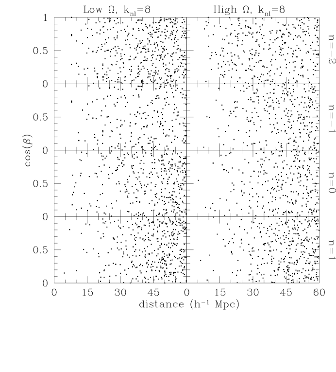
Figure 8: Figure 4 A scatter plot of cos $\beta$, the correlation angle for cluster pairs.

References

- [1]
- [2] Bahcall, N.A. 1988, ARAA, 26, 211
- [3]
- [4] Baier, F.W. 1983, Astron. Nacht., 5, 211
- [5]
- [6] Bahcall, & Cen, R. 1993, ApJ, 407, L49
- [7]
- [8] Batuski, D.J., Melott, A.L., & Burns, J.O. 1987, ApJ, 322, 48
- [9]
- [10] Beers, T.C., Forman, W., Huchra, J.P., Jones, C., Gebhardt, K. 1991, AJ, 102, 1581
- [11]
- [12] Binggeli, B. 1982, A&A, 107, 338
- [13]
- [14] Bird, C.M. 1993, Ph.D Thesis, University of Minnesota & Michigan State University
- [15]
- [16] Bird, C.M. 1994a AJ, 107, 1637
- [17]
- [18] Bird, C.M. 1994b ApJ, 422, 480
- [19]
- [20] Bond, J.R., Kofman, L. and Pogosan, D. 1996 Nature, 380, 003
- [21]
- [22] Carter, D., & Metcalfe, N. 1980, MNRAS, 191, 325
- [23]
- [24] Crone, M.M., Evrard, A.E., & Richstone, D.O. 1995, submitted to ApJ
- [25]
- [26] de Theije, P.A.M., Katgert, P., & van Kampen, E. 1995, MNRAS, 273,30
- [27]
- [28] Dressler, A. 1981, ApJ, 243, 26
- [29]
- [30] Dutta, S.N. 1995, submitted to MNRAS
- [31]
- [32] Efstathiou, G., Frenk, C., White, S.D.M., and Davis, M. 1988 MNRAS 235, 715
- [33]
- [34] Evrard, A.E., Mohr, J.J., Fabricant, D.G., & Geller, M.J. 1993, ApJ 419, L9
- [35]
- [36] Forman, W., Bechtold, J., Blair, R., Giacconi, R., Van Speybroeck, L., & Jones, C. 1981, ApJ, 243, L133
- [37]
- [38] Geller, M.J., & Beers, T.C. 1982, PASP, 94, 421
- [39]
- [40] Gregory, S.A., & Tifft, W.G. 1976, ApJ, 205, 716
- [41]
- [42] Henry, J.P., Henriksen, M., Charles, P. & Thorstensin, J., 1981 ApJ, 243, L137
- [43]
- [44] Hoessel, J.G., Gunn, J.E., & Thuan, T.X. 1980, ApJ, 241, 486
- [45]
- [46] Jones, C., & Forman, W. 1992 in Clusters and Superclusters of Galaxies, ed. A.C. Fabian, (Dordrecht: Kluwer), 49
- [47]
- [48] Kauffmann, G.A.M., & Melott, A.L. 1992, ApJ, 393, 415
- [49]
- [50] Kent, S.M., & Gunn, J.E. 1982, AJ, 87, 945
- [51]
- [52] Kent, S.M., & Sargent, W.L.W. 1983, AJ, 88, 697
- [53]
- [54] Melott, A.L., 1986, Phys Rev Lett, 56, 1992
- [55]
- [56] Melott, A.L. and Shandarin, S.F. 1993 ApJ, 410, 469
- [57]
- [58] Merritt, D. 1996 AJ submitted
- [59]
- [60] Mohr, J., Fabricant, D., & Geller, M.J. 1993, ApJ, 413, 492
- [61]
- [62] Pauls, J.L. and Melott, A.L. 1995, MNRAS, 274, 99
- [63]
- [64] Peebles, J.F., Melott, A.L., Holmes, M.R. and Jiang, L.R. 1989 ApJ, 345, 108
- [65]
- [66] Plionis, M. 1994, ApJS, 95, 401
- [67]
- [68] Plionis, M., Barrow, J.D., & Frenk, C.S. 1991, MNRAS, 249, 662
- [69]
- [70] Plionis, M. 1994, ApJS, 95, 401
- [71]
- [72] Praton, E. and Schneider, S.E. 1994, ApJ, 422, 46
- [73]
- [74] Press, W.H., Flannery, B.P., Teukolsky, S.A., & Vetterling, W.T. 1987, Numerical Recipes, (Cambridge: Cambridge University Press)
- [75]
- [76] Press, W.H., & Shechter, P. 1974, ApJ, 187, 425
- [77]
- [78] Rhee, G.F.R.N., and Katgert, P. 1987, A&A, 183, 217
- [79]
- [80] Rhee, G.F.R.N., van Haarlem, M., & Katgert, P. 1991a, AA, 246, 2
- [81]
- [82] Rhee, G.F.R.N., van Haarlem, M., & Katgert, P. 1991b, AA Suppl S, 91, 3
- [83]
- [84] Rhee, G.F.R.N., van Haarlem, M., & Katgert, P. 1992, AJ, 103, 1721
- [85]
- [86] Rhee, G.F.R.N., & Latour, 1991, AA, 243, 1
- [87]
- [88] Rood, H.J., Page, T.L., Kintner, E.C, King, I.R. 1972, ApJ, 175, 627
- [89]
- [90] Shandarin, S.F. and Klypin, A.A. 1984, Sov Astron, 28, 491
- [91]
- [92] Splinter, R.J., & Melott, A.L. 1996, in preparation
- [93]
- [94] Struble, M.F., & Peebles, P.J.E. 1985, AJ 90, 582
- [95]
- [96] Suisalu, I. and Saar, E. 1996, MNRAS, in press
- [97]
- [98] Summers, F.J., Davis, M. and Evrard, A.E. 1995, ApJ, 454, 1
- [99]
- [100] Tifft, W.G. 1980, ApJ, 239, 445
- [101]
- [102] van Haarlem, M., & van de Weygaert, R. 1993, ApJ, 418, 544
- [103]
- [104] Walter, C., & Klypin, A. 1996, ApJ, 462, 13
- [105]
- [106] West, M.J., Dekel, A., & Oemler A. 1989, ApJ, 336, 46
- [107]
- [108] West, M.J., Jones, C., & Forman, W. 1995, ApJ Lett, 451, L5
- [109]
- [110] West, M.J., Oemler, A., & Dekel, A. 1989, ApJ, 336, 46
- [111]
- [112] West, M.J. 1989a, ApJ, 344, 535
- [113]
- [114] West, M.J. 1989b, ApJ, 347, 610
- [115]
- [116] West, M.J., Villumsen J.V., & Dekel, A. 1991, ApJ, 369, 287
- [117]
- [118] White, S.D.M. 1996 to appear in proceedings of the 36th Hertmonceux Conference “Gravitational Dynamics” (eds. O. Lahav, E. Terlevich, and R. Terlevich).
- [119]
- [120] Zel’dovich, Ya. B. 1970, Astr Ap, 5, 84