One of the most powerful tools to probe the existence of cosmic defects in the early universe is through the Cosmic Microwave Background (CMB) radiation. It is well known that computations with causal sources are more involved than the adiabatic counterparts based on inflation, and this fact has in part hampered the development of fine detailed predictions. Analytical modeling, while necessarily limited in power, may tell us the overall characteristics of CMB from defects and hint at new features. We apply an analytical model for textures to the study of non–Gaussian features of the CMB sky and compare our predictions with the four–year COBE–DMR data.

To appear in Proceedings of the Moriond Conference on Microwave Background Anisotropies, March 16th–23rd 1996

1 Introduction

It has by now become clear that one of the most promising ways to learn about the early universe is through the Cosmic Microwave Background (CMB) radiation. With the prospective launch of future missions, like MAP and COBRAS/SAMBA, one can hope that many of the so far elusive cosmological parameters will be pinned down with unprecedent precision. The four–year COBE plus other large–scale structure data have placed strong constraints on current models of structure formation. However the remaining window is still too large and many (widely) different cosmological models pass the test. This is actually the case with cosmic defect theories, on the one hand and inflation–based adiabatic models on the other.

The search for the so–called Doppler peaks (or Sakharov peaks if you like) seems to be among the first goals for next generation detectors, the aim being in trying to discriminate among, say, standard adiabatic CDM models¹⁾, cosmic strings²⁾ and textures³⁾. Whereas the generation of CMB anisotropies seems to be fully understood within adiabatic models [refer to Hu’s contribution to these proceedings], the same does not happen for the latter models, where the non–linear evolution of the defects and their active role in seeding anisotropies in the CMB makes the analysis far more involved [see Durrer’s contribution]. Moreover, causal sources can produce spectra mimicking the outcome of inflationary models⁴⁾, hence increasing the uncertainty and calling for fast and accurate methods for computing the theoretical predictions [Seljak’s contribution], and refined experiments to confront these competing theories.

Other means of narrowing somewhat the window regards the recognition that the CMB radiation carries valuable information of the processes that generated the anisotropies, all along the path of the photons from the last scattering surface to our present detectors: should future experiments find (with high confidence level) a departure of the statistics of the anisotropies from Gaussianity, it would disfavor the standard inflaton field quantum fluctuation origin of the cosmological perturbations. It then follows that it is interesting to calculate what predictions cosmic defects make regarding non–Gaussian features in the CMB sky. It is the aim of this short contribution to report on some work done on the CMB three–point correlation function predicted by textures within a simple analytical model.

2 The model

Magueijo⁵⁾ recently proposed a simple analytical model for the computation of the ${\cal C}_{\ell}$’s from textures. The model exploits the fact that in this scenario the microwave sky will show evidence of spots due to perturbations in the effective temperature of the photons resulting from the non–linear dynamics of concentrations of energy–gradients of the texture field. The model of course does not aim to replace the full range numerical simulations but just to show overall features predicted by textures in the CMB anisotropies. In fact the model leaves free a couple of parameters that are fed in from numerical simulations, like the number density of spots, $\nu$, the scaling size, $d_{s}$, and the brightness factor of the particular spot, $a_{k}$, telling us about its temperature relative to the mean sky temperature.

Texture configurations giving rise to spots in the CMB are assumed to arise with a constant probability per Hubble volume and Hubble time. In an expanding universe one may compute the surface probability density of spots

$$dP=N(y)dyd\Omega,\quad\mbox{with}\quad N(y)=-{8\nu\ln(2)\over 3}\left(2^{y/3}-1\right)^{2},$$ (1)

where $\Omega$ stands for a solid angle on the two–sphere and the time variable $y(t)\equiv\log_{2}(t_{0}/t)$ measures how many times the Hubble radius has doubled since proper time $t$ up to now.

In the present context the anisotropies arise from the superposition of the contribution coming from all the individual spots $S_{k}$ produced from $y_{\rm ls}$ up to now, and so, $\Delta T/T=\sum_{k}a_{k}S_{k}(\theta_{k},y)$, where the random variable $a_{k}$ stands for the brightness of the hot/cold $k$–th spot with characteristic values to be extracted from numerical simulations⁶⁾. $S_{k}(\theta_{k},y)$ is the characteristic shape of the spots produced at time $y$, where $\theta_{k}$ is the angle in the sky measured with respect to the center of the spot. A spot appearing at time $y$ has typically a size $\theta^{s}(y)\simeq d_{s}~{}\theta^{\rm hor}(y)$, with $\theta^{\rm hor}(y)$ the angular size of the horizon at $y$, and where it follows that $\theta^{s}(y)=\arcsin\left({0.5d_{s}\over 2^{y/3}-1}\right)$. Textures are essentially causal seeds and therefore the spots induced by their dynamics cannot exceed the size of the horizon at the time of formation, hence $d_{s}\leq 1$. Furthermore the scaling hypothesis implies that the profiles satisfy $S_{k}(\theta_{k},y)=S(\theta_{k}/\theta^{s}(y))$. From all this it follows a useful expression for the multipole coefficients, $a_{\ell}^{m}=\sum_{k}a_{k}S^{\ell}_{k}(y){Y_{\ell}^{m}}^{*}(\hat{\gamma}_{k})$, with $S^{\ell}_{k}(y)$ the Legendre transform of the spot profiles.

At this point the ${\cal C}_{\ell}$’s are easily calculated⁵⁾. As we are mainly concerned with the three–point function we go on and compute the angular bispectrum predicted within this analytical model, which we find to be

$$\bigl{\langle}a_{\ell_{1}}^{m_{1}}a_{\ell_{2}}^{m_{2}}a_{\ell_{3}}^{m_{3}}\bigr{\rangle}=\bigl{\langle}a^{3}\bigr{\rangle}\int dyN(y)S^{\ell_{1}}(y)S^{\ell_{2}}(y)S^{\ell_{3}}(y)\int d\Omega_{\hat{\gamma}}Y_{\ell_{1}}^{m_{1}}(\hat{\gamma})Y_{\ell_{2}}^{m_{2}}(\hat{\gamma})Y_{\ell_{3}}^{m_{3}}(\hat{\gamma}).$$ (2)

$\bigl{\langle}a^{3}\bigr{\rangle}$ is the mean cubic value of the spot brightness.

Having the expression for the bispectrum we may just plug it in the formulae for the full mean three–point temperature correlation function⁷⁾. To make contact with experiments however we restrict ourselves to the collapsed case where two out of the three legs of the three–point function collapse and only one angle, say $\alpha$, survives (this is in fact one of the cases analyzed for the four–year COBE–DMR data⁸⁾).

The collapsed three–point function thus calculated, $\bigl{\langle}C_{3}(\alpha)\bigr{\rangle}$, corresponds to the mean value expected in an ensemble of realizations. However, as we can observe just one particular realization, we have to take into account the spread of the distribution of the three–point function values when comparing a model prediction with the observational results. This is the well–known cosmic variance problem. We can estimate the range of expected values about the mean by the rms dispersion $\sigma_{CV}^{2}(\alpha)\equiv\bigl{\langle}C_{3}^{2}(\alpha)\bigr{\rangle}-\bigl{\langle}C_{3}(\alpha)\bigr{\rangle}^{2}$. We will estimate the range for the amplitude of the three–point correlation function predicted by the model by $\bigl{\langle}C_{3}(\alpha)\bigr{\rangle}\pm\sigma_{CV}(\alpha)$.

It has been shown⁶⁾ that spots generated from random field configurations of concentrations of energy gradients lead to peak anisotropies 20 to 40 % smaller than those predicted by the spherically symmetric self–similar texture solution. These studies also suggest an asymmetry between maxima $\langle a_{\rm max}\rangle$ and minima $\langle a_{\rm min}\rangle$ of the peaks as being due to the fact that, for unwinding events, the minima are generated earlier in the evolution (photons climbing out of the collapsing texture) than the maxima (photons falling in the collapsing texture), and thus the field correlations are stronger for the maxima, which enhance the anisotropies.

3 Results

Let us now compute the predictions on the CMB non–Gaussian features derived from the present analytical texture model. One needs to have the distribution of the spot brightness $\{a_{k}\}$ in order to compute the mean values $\langle a^{n}\rangle$. It is enough for our present purposes to take for all hot spots the same $a_{h}>0$ and for all the cold spots the same $a_{c}<0$. Then the $\langle a^{n}\rangle$ needed can readily be obtained in terms of $\langle a^{2}\rangle$ and $x\equiv\langle a\rangle/\langle|a|\rangle$. We fix $\langle a^{2}\rangle$ from the amplitude of the anisotropies according to four–year COBE–DMR⁸⁾. The other parameter, $x$, that measures the possible asymmetry between hot and cold spots, we leave as a free parameter.

We consider the COBE–DMR window function and, in order to take into account the partial sky coverage due to the cut in the maps at Galactic latitudes $|b|<20^{\circ}$, we multiply $\sigma_{CV}$ by a factor $\sim 1.5$ in the numerical results (sample variance).

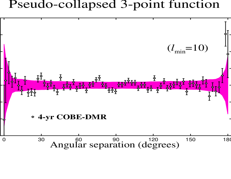
Figure 1: The ‘pseudo–collapsed’ three–point function (in units of $10^{4}{\mu}{\rm K}^{3}$) as computed from the analysis of the four–year COBE–DMR data [data courtesy of G. Hinshaw and the COBE team]. The points plotted are the analogue of our $\bigl{\langle}C_{3}(\alpha)\bigr{\rangle}$. Error bars represent instrument noise while the grey band represents the rms range of fluctuations due to a superposition of instrument noise and cosmic variance.

Let us now compare with the data: Subtracting the dipole and for all reasonable values of the asymmetry parameter $x$, the data falls well within the $\bigl{\langle}C_{3}(\alpha)\bigr{\rangle}\pm\sigma_{CV}(\alpha)$ band, and thus there is good agreement with the observations. However, the band for Gaussian distributed fluctuations (e.g., as predicted by inflation) also encompasses the data well enough, and it is in turn included inside the texture predicted band. The fact that the range of expected values for the three–point correlation function predicted by inflation is included into that predicted by textures for all the angles, and that the data points fall within them, makes it impossible to draw conclusions favoring one of the models.

It is well known that the largest contribution to the cosmic variance comes from the small values of $\ell$. Thus, no doubt the situation may improve if one subtracts the lower order multipoles contribution, as in a $\ell_{min}=10$ analysis⁹⁾. In Figure 1 we show the analysis of the four–year COBE–DMR data evaluated from the 53 + 90 GHz combined map, containing power from the $\ell=10$ moment and up. It is apparent that the fluctuations about zero correlation (i.e., no signal) are too large for the instrument noise to be the only responsible. These are however consistent with the range of fluctuations expected from a Gaussian process (grey band).

What we want to see now is whether our analytical texture model for the three–point function¹⁰⁾ can do better when compared with the data. Figure 2 shows the collapsed three–point function $\bigl{\langle}C_{3}(\alpha)\bigr{\rangle}$ (solid line) and the grey band indicates the rms range of fluctuations expected from the cosmic variance. Also shown is a black band with the expected range for inflationary models (no instrument noise included). The bands do not superpose each other for some ranges of values of the separation angle for the value of $x=0.4$ considered, what means that measurements in that ranges can distinguish among the models. The value of the parameter $x$ considered is quite in excess of that suggested by simulations⁶⁾, but was chosen to show an example with a noticeable effect.

Figure 2: Expected range of values for the three–point correlation function for the texture model with asymmetry parameter $x=0.4$ (grey band). Also shown is the expected range for inflationary models (black band). Both bands include the $\sim 50\%$ increase in $\sigma_{CV}$ due to the sample variance. All multipoles up to $\ell=9$ have been subtracted. The right panel shows a zoomed fraction of the same plot.

In Figure 3 we show the result of combining the previous figures, confronting the actual data with the curves predicted by the texture model.

Figure 3: Combined four–year COBE–DMR data and collapsed three–point correlation function predicted by the analytical texture model (as in previous figures). Left panel: for a somewhat exaggerated value of the asymmetry parameter $x=0.4$. Right panel: for the value $x\sim 0.1$ suggested by texture simulations.

From these figures one may see qualitatively by eye that (for some ranges of the angular separation better than for others, of course) the data seems to follow ‘approximately’ the trend of the texture curves. While many of the data points fell outside the Gaussian band (Figure 1), most of them are now inside the grey band in Figure 3 (left panel). Moreover, while we vary the $x$ values from 0.4 down to 0.1 (the actual value suggested by texture simulations) we see that more and more points (with error bars) get inside (or touch) the grey band. Can this be just by chance? Or is it there something worth of further study? In order to answer these questions one ought to quantify more the analysis by using a $\chi^{2}$ statistics for the model and data, and comparing it to the Gaussian case, e.g.¹¹⁾

$$\chi^{2}=\sum_{\alpha\beta}(D_{\alpha}-\bigl{\langle}C_{3}\bigr{\rangle}_{\alpha})({\rm M}^{-1})_{\alpha\beta}(D_{\beta}-\bigl{\langle}C_{3}\bigr{\rangle}_{\beta}),$$ (3)

with $D_{\alpha}$ the COBE–DMR three–point function and ${\rm M}$ is the covariance matrix of the analytical model. It might be that the data picks out a preferred value for the asymmetry parameter $x$. Work in this direction is currently under way.

Acknowledgments: I thank Gary Hinshaw and the COBE team for providing the 4-yr data, and especially Gary for useful correspondence. I also thank Silvia Mollerach for her collaboration on the work described herein, Ruth Durrer, Andrew Liddle and Neil Turok for useful conversations during the workshop, and the organizers for making this such a stimulating meeting. I acknowledge partial funding from The British Council/Fundación Antorchas.

References

1. W. Hu, N. Sugiyama and J. Silk, astro-ph/9604166.
2. A. Albrecht, D. Coulson, P. Ferreira and J. Magueijo, Phys. Rev. Lett. 76, 1413 (1996); see also Hobson’s contribution to these proceedings.
3. R. G. Crittenden and N. Turok, Phys. Rev. Lett. 75, 2642 (1995); R. Durrer, A. Gangui and M. Sakellariadou, Phys. Rev. Lett. 76, 579 (1996).
4. N. Turok, astro-ph/9604172.
5. J. Magueijo, Phys. Rev. D 52, 689 (1995).
6. J. Borrill, E. Copeland, A. Liddle, A. Stebbins and S. Veeraraghavan, Phys. Rev. D. 50, 2469 (1994).
7. A. Gangui, F. Lucchin, S. Matarrese and S. Mollerach, Astrophys. J. 430, 447 (1994).
8. E. W. Wright, C. L. Bennett, K. M. Górski, G. Hinshaw and G. F. Smoot, astro-ph/9601059.
9. G. Hinshaw, A. J. Banday, C. L. Bennett, K. M. Górski and A. Kogut, Astrophys. J. 446, L67 (1995).
10. A. Gangui and S. Mollerach, astro-ph/9601069.
11. A. Kogut, A. J. Banday, C. L. Bennett, K. Górski, G. Hinshaw, G. F. Smoot and E. L. Wright, astro-ph/9601062.