Abstract

Cosmic strings provide a radically different paradigm for the formation of structure to the prevailing inflationary one. They afford some extra technical complications: for example, the calculation of the power spectrum of matter and radiation perturbations requires the knowledge of the history of the evolution of the defects in the form of two-time correlation functions. We describe some numerical simulations of string networks, designed to measure the two-time correlations during their evolution.

COSMIC STRINGS AND COHERENCE

¹ School of Mathematical and Physical Sciences, University of Sussex, Brighton BN1 9QH, U.K. ² Département de Physique Théorique, Université de Genève, Quai Ernest-Ansermet 24, CH-1211 Genève 4, Switzerland

1 Introduction

Calculations of the Cosmic Microwave Background (CMB) fluctuations from cosmic strings [1] have proved much harder than their inflationary equivalents. One of the reasons is that the energy-momentum of the defects cannot be considered to be a perfect fluid like most of the rest of the contents of the Universe: instead we have to use numerical simulations to find how important quantities such as the energy density and velocity evolve. The defect energy-momentum is then a source for perturbations in the gravitational field, which must be calculated either using Greens functions [2] or by direct numerical integration [3].

A major problem with using numerical simulations is the lack of dynamic range, even with supercomputers. The largest simulations can only span a ratio of conformal times of about 10, which is not totally satisfactory. For calculating simple quantities such as power spectra an alternative approach is available: to use numerical simulations to construct an accurate model of the appropriate source functions, which are two-time correlation functions of various components of the energy-momentum tensor. Relatively simple Greens functions can then be used to compute the power spectra of perturbations in perfect fluids, including CDM and tightly coupled photons and baryons.

This talk summarises some work in progress [4] on the properties of cosmic strings as sources of the gravitational perturbations. An issue of interest which we address is that of coherence, recently raised in [5], and explored in more detail by the same authors in [6].

2 Perturbations from defects

A simple model serves to illustrate the issues involved. We suppose that the Universe is spatially flat with zero cosmological constant, and consists of Cold Dark Matter (CDM), photons, baryons, and defects, with average densities $\rho_{c}$, $\rho_{\gamma}$, $\rho_{B}$ and $\rho_{s}$ respectively. The fluid density perturbations are written $\delta_{c}$, $\delta_{\gamma}$, $\delta_{B}$ and the velocity perturbations are $\mbox{\boldmath$v$}_{c}$, $\mbox{\boldmath$v$}_{\gamma}$, $\mbox{\boldmath$v$}_{B}$. The defect energy-momentum tensor is $\Theta_{\mu\nu}$, which is also a small perturbation to the background, and to first order can be considered separately conserved (or stiff [2]). We take the synchronous gauge. Before decoupling at a redshift of $z_{\rm rec}\simeq 1100$ (assuming the standard ionization history), the photons and baryons were tightly coupled by Thompson scattering, which forces $\delta_{B}=\frac{3}{4}\delta_{\gamma}$ and $\mbox{\boldmath$v$}_{B}=\mbox{\boldmath$v$}_{\gamma}$.

It is very convenient to use an entropy $s=(\frac{3}{4}\delta_{\gamma}-\delta_{c})$, and its time derivative $\dot{s}$, which is equal to the divergence of the radiation peculiar velocity. It is also convenient to introduce the pseudoenergy $\tau_{00}$ [2], which is part of an ordinarily conserved energy-momentum pseudotensor:

$$\tau_{00}=\Theta_{00}+\frac{3}{8\pi G}\left(\frac{\dot{a}}{a}\,\right)^{2}(\Omega_{c}\delta_{c}+\Omega_{\gamma}(1+R)\delta_{\gamma})+\frac{1}{4\pi G}\left(\frac{\dot{a}}{a}\,\right)\dot{\delta}_{c},$$ (1)

where $R=3\rho_{B}/4\rho_{\gamma}$. In the sychronous gauge the pseudo-energy is in fact proportional to the scalar curvature of the constant conformal time slices.

Let us now define the pseudo-energy perturbation

$$\delta_{00}=\frac{8\pi G}{3}\left(\frac{a\,}{\dot{a}}\right)^{2}\tau_{00}.$$ (2)

We may use the conservation equations for the defects to write the equations of motion of the fluids as four first-order equations [3]

$$\dot{\delta}_{c} = \frac{3}{2}\left(\frac{\dot{a}}{a}\,\right)[\delta_{00}-(\Omega_{c}+2\Omega_{\gamma}(1+R))\delta_{c}-2\Omega_{\gamma}(1+R)s]-\mbox{\boldmath${\displaystyle\frac{3}{2}\left(\frac{\dot{a}}{a}\,\right)\Omega_{s}\delta_{s}}$},$$ (3)

$$\dot{s} = y,$$ (4)

$$\dot{\delta}_{00} = \left(\frac{\dot{a}}{a}\,\right)(1+3w)\delta_{00}+\frac{4}{3}\Omega_{\gamma}(1+R)y+\mbox{\boldmath${\displaystyle\Omega_{s}kv_{s}}$},$$ (5)

$$\dot{y} = -k^{2}c_{s}^{2}(s+\delta_{c})-\left(\frac{\dot{a}}{a}\,\right)(1-3c_{s}^{2})y,$$ (6)

where $w=p/\rho$, the ratio of the total pressure to the total energy density, and $c_{s}^{2}=1/3(1+R)$.

These equations have the inhomogeneous form $\dot{\Delta}_{i}=M_{i}^{j}\Delta_{j}+\Sigma_{i}$, where $\Delta=(\delta_{c},s,\delta_{00},y)^{T}$, and the source vector, picked out in bold above, is $\Sigma=(-\frac{3}{2}(\dot{a}/a)\Omega_{s}\delta_{s},\;0,\;\Omega_{s}kv_{s},\;0)^{T}$. The solution to these equations with initial condition $\Delta(\eta_{i})$ is then

$$\Delta(\eta)=G(\eta,\eta_{i})\Delta(\eta_{i})+\int_{\eta_{i}}^{\eta}\,d\eta^{\prime}G(\eta,\eta^{\prime})\Sigma(\eta^{\prime}),$$ (7)

where $G(\eta,\eta^{\prime})$ is the Green’s function. The initial perturbation is $\Delta(\eta_{i})=(\delta_{c}(\eta_{i}),0,0,0)^{T}$, corresponding to perturbations which are both adiabatic, in the sense that $s=0$, and isocurvature, in the sense that $\tau_{00}=0$. In the presence of defects, the isocurvature condition forces the initial perturbations in the matter and radiation to compensate those of the defects. However, the initial compensation can be ignored, as the initial condition consists only of decaying modes, which is one of the advantages of using this basis for the perturbations [3]. An initial condition consisting purely of adiabatic growing modes would be $\Delta(\eta_{i})=(\delta_{c}(\eta_{i}),0,2\delta_{c}(\eta_{i}),0)^{T}$.

At time $\eta$, the power spectra of the various perturbations are therefore

$$\langle|\Delta_{i}(\eta)|^{2}\rangle=\int_{\eta_{i}}^{\eta}\,d\eta_{1}\int_{\eta_{i}}^{\eta}\,d\eta_{2}G_{i}^{j}(\eta,\eta_{1})G_{i}^{k}(\eta,\eta_{2})\langle\Sigma_{j}(\eta_{1})\Sigma_{k}^{*}(\eta_{2})\rangle,$$ (8)

(no sum on $i$). It is clear from this equation that the calculation of the power spectra requires the knowledge of the two-time correlation functions

$$C^{\rho\rho}(\eta_{1},\eta_{2})=\langle\delta_{s}(\eta_{1})\delta_{s}^{*}(\eta_{2})\rangle,\quad C^{UU}(\eta_{1},\eta_{2})=\langle v_{s}(\eta_{1})v_{s}^{*}(\eta_{2})\rangle,\quad X^{\rho U}(\eta_{1},\eta_{2})=\langle\delta_{s}(\eta_{1})v_{s}^{*}(\eta_{2})\rangle,$$ (9)

where the angle brackets are to be understood as averages over ensembles of topological defects.

3 Flat space cosmic string simulations

In order to compute the averages in (9) we performed many simulations of networks of string in Minkowski space [7, 8]. It is not at first sight such a good idea to abandon the expanding Universe, but there are arguments which support the procedure. Firstly, a spatially flat FRW cosmology is conformal to Minkowksi space, so one can identify Minkowksi time with conformal time, and Minkowksi space coordinates with comoving space coordinates. Secondly, the string network scale length is significantly smaller than the horizon length, which means that the effects of the expanding background on the dynamics of the string should be small. Thirdly, a string network can be well described by a couple of parameters: the string density and the correlation length of the network [9], which means we can hope to translate Minkowksi space results into FRW results by appropriate scalings. Lastly, the savings in computational resources are immense. The strings can be evolved on a cubic spatial lattice, which means that only integer arithmetic need be used, and that self-intersections are extremely easy to check for.

A vital property possessed by string networks is known as scaling. In its simplest form, scaling means that all quantities with dimensions of length are proportional to a fundamental network scale $\xi$, which is in turn a function of length scales in the network dynamics. In a cosmological setting, the only scale in the equations of motion is the horizon or the conformal time $\eta$. Thus $\xi\propto\eta$, where $\xi$ is understood to be a comoving scale. The invariant length density $\L$ (which is proportional to the energy density through the string mass per unit length $\mu$) is therefore, on naive dimensional grounds, proportional to $\xi^{-2}$. In fact, it is convenient to define $\xi$ by $\xi=1/\sqrt{\L}$. The simulations conserve energy and thus invariant length. However, real strings decay into particles and gravitational radiation, so we model this by excluding small loops below a threshold $l_{c}$ from being counted as string. This threshold may be chosen in many ways: it can be a constant, or it may be a fixed fraction of $\xi$. However, we find that the remainder (“long” or “infinite” string) always scales towards the end of the simulations, that is, $\xi=x\eta$, although the constant $x$ depends on how the cut-off is chosen.

Scaling has important implications for the correlation functions. For example, the correct scaling behaviour for the power spectrum of the string density is

$$C^{\rho\rho}(\eta,\eta)=\frac{1}{\xi}P^{\rho}(k\xi).$$ (10)

We can also express the velocity power spectrum in terms of a similar scaling function $P^{U}(k\eta)$. These forms ensure that the mean square fluctuation in the string density at horizon crossing is constant, when $\xi/\eta$ is constant. Hence the compensating fluctuations in the matter and radiation are also constant at horizon crossing, which gives a Harrison-Zel’dovich spectrum.

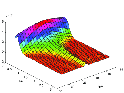
Figure 1: Two-time correlation function $\langle{\Theta_{00}(k,\eta)\Theta_{00}^{*}(k,\eta^{\prime})\rangle}$ for $\eta^{\prime}=22\delta$

In Figures 1, 2, and 3 the correlation functions (9) measured for strings whose length is above the threshold $l_{c}$ are displayed. They result from many simulations on $(64\delta)^{3}$ or $(128\delta)^{3}$ lattices, where $\delta$ is the lattice spacing, with approximately $7500$ or $60000$ string points. For calculating the two-time correlation functions we typically averaged over 50 simulations. We find that good fits in the important regions where the correlators are large are obtained from the following functions

$$C^{\rho\rho} = {1\over\sqrt{\xi\xi^{\prime}}}\sqrt{P^{\rho}(k\xi)P^{\rho}(k\xi^{\prime})}{\it e}^{-{\frac{1}{2}}\Upsilon^{2}k^{2}(1-(k\Delta))(\eta-\eta^{\prime})^{2}}$$ (11)

$$C^{\rho U} = {1\over\sqrt{\xi\xi^{\prime}}}\sqrt{P^{\rho}(k\xi)P^{\rho}(k\xi^{\prime})}{\it e}^{-{\frac{1}{2}}\Upsilon^{\prime 2}k^{2}(\eta-\eta^{\prime})^{2}}({\alpha\over k\sqrt{\xi\xi^{\prime}}}-\Upsilon^{\prime 2}k(\eta-\eta^{\prime}))$$ (12)

$$C^{UU} = {1\over\sqrt{\xi\xi^{\prime}}}\sqrt{P^{U}(k\xi)P^{U}(k\xi^{\prime})}{\it e}^{-{\frac{1}{2}}\Upsilon^{\prime\prime 2}k^{2}(\eta-\eta^{\prime})^{2}}(1-\Upsilon^{\prime\prime 2}k^{2}(\eta-\eta^{\prime})^{2})$$ (13)

The values for $\Upsilon$, $\Upsilon^{\prime}$ and $\Upsilon^{\prime\prime}$ are given in Table 3. $\Delta$ is approximately $3\delta$, which indicates that it is probably a lattice artifact.

Table 1. The values of the parameters for the models in equations (11), (12) and (13), obtained by minimising the $\chi^{2}$.

$l_{c}$	$\Upsilon$	$\alpha$	$\Upsilon^{\prime}$	$\Upsilon^{\prime\prime}$
$2\delta$	$0.21\pm 0.05$	$0.19\pm 0.05$	$0.42\pm 0.05$	$0.36\pm 0.07$
$4\delta$	$0.18\pm 0.05$	$0.16\pm 0.05$	$0.42\pm 0.05$	$0.42\pm 0.06$

Figure 2: Two-time correlation function $\langle{U(k,\eta)\Theta_{00}^{*}(k,\eta^{\prime})\rangle}$ for $\eta^{\prime}=22\delta$

4 Implications for strings in FRW backgrounds

The effect of the expansion of the Universe in a Friedmann model is to reduce the velocity string segments by Hubble damping, just as for particles. However, as the string moves relativistically, the equation of motion becomes non-linear. The conservation equations for $\Theta_{00}$ and $U=i\hat{k}_{i}\Theta_{0i}$ become

$$\dot{\Theta}_{00}+\frac{\dot{a}}{a}\,(\Theta_{00}+\Theta)+kU = 0,$$ (14)

$$\dot{U}+2\frac{\dot{a}}{a}\,U+\frac{1}{3}k(\Theta+2\Theta^{\rm s}) = 0,$$ (15)

where $\Theta\equiv\Theta_{ii}$ and $\Theta^{\rm s}\equiv(\hat{k}_{i}\hat{k}_{j}-\frac{1}{3}\delta_{ij})\Theta_{ij}$. Both $\Theta$ and $\Theta^{\rm s}$ are unconstrained by energy-momentum conservation, and so one could imagine that fluctuations in the pressure could drive extra fluctuations in the energy density through the second term in (14). As the scale of this term is $\eta^{-1}$ rather than $k$, this could change the conclusions of the previous section, that the coherence time for a mode of wavenumber $k$ was proportional to $k^{-1}$. Instead we could have the situation assumed in [5], with coherence time proportional to $\eta$. Outside the horizon, this makes a significant difference.

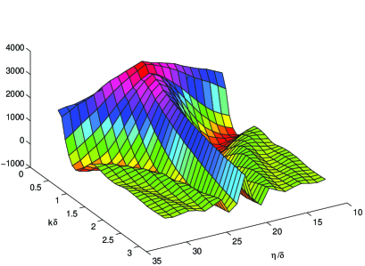
Figure 3: Two-time correlation function $\langle{U(k,\eta)U^{*}(k,\eta^{\prime})\rangle}$ for $\eta^{\prime}=22\delta$

Let us examine how this might work, for superhorizon modes ($k\eta\ll 1$). Firstly, we divide $\Theta_{00}$ and $\Theta$ into coherent and incoherent parts:

$$\Theta_{00}=\bar{\Theta}_{00}+\Delta_{00},\qquad\Theta=3w_{s}\bar{\Theta}_{00}+r,$$ (16)

where $r$ is a random variable, whose fluctuations are limited only by the requirement of scale invariance. Thus

$$\langle r(\eta_{1})r^{*}(\eta_{2})\rangle=\frac{1}{\sqrt{\eta_{1}\eta_{2}}}R(\eta_{1}/\eta_{2}).$$ (17)

It is then not hard to show that energy-momentum conservation implies that

$$\langle|\Delta_{00}|^{2}\rangle\sim\langle|r|^{2}\rangle.$$

Since $\langle|r|^{2}\rangle<\langle|\Theta|^{2}\rangle$, the extra fluctuations in the density induced by the pressure term are controlled by the size of the pressure term. Now, in the Minkowski space simulations, we find that $\langle|\Theta|^{2}\rangle\sim 0.1\langle|\Theta_{00}|^{2}\rangle$ for $k\eta\ll 1$, and thus we argue that any extra fluctuations in Friedmann models, with a coherence time set by the horizon $\eta$, are likely to be small.

5 Conclusions

We have taken the first steps on the road to calculating the matter and radiation power spectra in the cosmic string scenario, by constructing a realistic model of the important parts of the string energy-momentum tensor which drive the fluid perturbations. We have argued that the Minkowski space simulations we used to construct the model incorporates the essential features of string evolution in an expanding universe, and that corrections due to the expansion are small. This of course should be checked with FRW string codes. Perhaps the most important feature of the string network is its coherence time, the time over which the phases of the Fourier components of the string energy-momentum tensor are correlated. We find that there is no single coherence time for the whole network. Although the fall-off away from the equal-time value is modulated by functions whose dominant behaviour is $\exp(-(\eta_{1}-\eta_{2})^{2}/2\eta_{c}^{2})$, and the scale is set by $k^{-1}$ for each mode, $\eta_{c}$ is different for different correlation functions.

Acknowledgements.  GRV and MBH are supported by PPARC, by studentship number 94313367, Advanced Fellowship number B/93/AF/1642 and grant number GR/K55967. MS is supported by the Tomalla Foundation. Partial support is also obtained from the European Commission under the Human Capital and Mobility programme, contract no. CHRX-CT94-0423.

References

- [1] Hindmarsh M. and Kibble T.W.B.. 1995, Rep. Prog. Phys 58 477
- [2] Veeraraghavan S. and Stebbins A., 1990, Astrophys. J. 365, 37
- [3] Pen U.L., Spergel D.N. and Turok N., 1994, Phys. Rev. D49 692
- [4] Vincent G., Hindmarsh M. and Sakellariadou M., 1996, Correlations in Cosmic String Networks astro-ph/9606137
- [5] Albrecht A., Coulson D., Ferreira P. and Magueijo J., 1996, Phys. Rev. Lett. 76 1413
- [6] Magueijo J., Albrecht A., Coulson D. and Ferreira P., 1996, MRAO-1917 astro-ph/9605047
- [7] Smith A.G. and Vilenkin A., 1987, Phys. Rev. D36, 990
- [8] Sakellariadou M. and Vilenkin A., 1988, Phys. Rev. D37, 885
- [9] Copeland E.J., Kibble T.W.B. and Austin D., 1992, Phys. Rev. D45 R1000