The 6 cm Light Curves of B0957+561, 1979-1994:
New Features and Implications for the Time Delay

Abstract

We report on 15 years of VLA monitoring of the gravitational lens B0957+561 at 6 cm. Since our last report in 1992, there have been 32 additional observations, in which both images have returned to their quiescent flux density levels and the A image has brightened again. We estimate the time delay from the light curves using three different techniques: the $\chi^{2}$ analysis of Press, Rybicki, & Hewitt (1992a,b), the dispersion analysis of Pelt et al. (1994, 1996), and the locally normalized discrete correlation function of Lehár et al. (1992). Confidence intervals for these time delay estimates are found using Monte Carlo techniques. With the addition of the new observations, it has become obvious that five observations from Spring 1990 are not consistent with the statistical properties of the rest of the light curves, so we analyze the light curves with those points removed, as well as the complete light curves. The three statistical techniques applied to the two versions of the data set result in time delay values in the range 398 to 461 days (or 1.09 to 1.26 years, A leading B), each with $\sim$5% formal uncertainty. The corresponding flux ratios (B/A) are in the range 0.698 to 0.704. Thus, the new features in the light curve show that the time delay is less than 500 days, in contrast with analysis of earlier versions of the radio light curves. The large range in the time delay estimates is primarily due to unfortunate coincidences of observing gaps with flux variations.

1 Introduction

With the discovery of the double quasar B0957+561 in 1979 (Walsh, Carswell, & Weymann (1979)), the door was opened for observational cosmology using gravitational lenses. Lenses offer the possibility of determining angular diameter distances at large redshifts, independent of the assumptions that underlie other distance measurement techniques. The time delay between pairs of lensed images of a variable source, when combined with a model of the lensing potential, gives an estimate of angular diameter distance, and thus constrains the Hubble parameter $H_{0}$, the deceleration $q_{0}$, and the cosmological constant $\Lambda_{o}$ (Refsdal 1964, 1966; Narayan (1991)). Since cosmological parameters other than $H_{0}$ affect the time delay, measurements of many lensed systems at various redshifts will ultimately be needed. The possibilities for B0957+561 were realized immediately, and VLA and optical monitoring for the time delay began in 1979.

Table 1 lists measurements of the time delay of B0957+561, showing the literature reference, light curves, and estimate of the time delay in days and in years. Note that before 1989 the results were scattered in delay, with large errors. More recently, estimates for the delay have clustered around 415 days and 540 days. Before 1992 it seemed that the optical light curves gave shorter delays and the radio light curves gave longer delays, and since 1992 a variety of analyses have been used on the light curves in attempts to resolve the discrepancy. Although some statistical techniques have found consistent delays at optical and radio wavelengths, the techniques have not been consistent with each other. The statistical properties of the noisy irregularly sampled light curves (complicated by microlensing effects at optical wavelengths) have proven difficult to understand, and the conclusion has often been that more observations are needed. We present here lengthened radio light curves with additional features.

Although the ultimate goal of this project is to determine the angular diameter distance to the lens, we focus this paper primarily on the value of the time delay and techniques for measuring it accurately. Determining $H_{0}$ from the time delay requires assumptions about $q_{0}$ and $\Lambda_{0}$, and a good model of the lensing potential, in itself a subject of much recent work (Grogin & Narayan 1996a, 1996b; Bernstein, Tyson, & Kochanek (1993); Falco, Gorenstein, & Shapiro (1991); Kochanek (1991)). Recent observations have provided an improved understanding of the cluster and galaxy lensing potentials (Garrett et al. (1994); Angonin-Willaime, Soucail, & Vanderriest (1994); Dahle, Maddox, & Lilje (1994); Fischer et al. (1996); Falco et al. (1996)), which should allow for better constrained models.

In addition to the time delay, the light curves give the flux ratio between the A and B images, an important parameter in lens modeling. Since the lensing effect is achromatic, this relative magnification is independent of wavelength, as long as the emission region size is also independent of wavelength and the angular resolution of the observations is comparable. These conditions are not met when comparing the VLA flux ratio to the optical flux ratio, since the optical emission region is much smaller than the 6 cm emission region. The VLA flux ratio will also differ from the VLBI ratio, since the VLA beam averages over the varying magnification on mas scales (Conner, Lehár, & Burke (1992)). All flux ratios reported here are ratios between the VLA 6 cm images of A and B.

It is four years since our last report on the VLA 6 cm monitoring of B0957+561. Preliminary results on the most recent data have been released (Haarsma et al. 1995a ; Haarsma et al. 1995b ); here we provide the complete data and results of 15 years of observations. New features have appeared that allow us to improve our estimate of the time delay. To determine the time delay, we have chosen three of the techniques referred to in Table 1: PRH$\chi^{2}$ analysis (Press, Rybicki, & Hewitt, 1992a,b, hereafter PRHa, PRHb; Rybicki & Press (1992); Rybicki & Kleyna (1994)), dispersion analysis (Pelt et al. 1994, Pelt et al. 1996, hereafter P94, P96), and discrete correlation function analysis (Lehár et al. 1992, hereafter L92; Edelson & Krolik (1988)). These were selected to provide consistency with our previous work and to explore an additional technique. All three avoid interpolation of the light curve, a practice that biases the result for irregularly sampled data by weighting assumed data during observing gaps the same as real observations (Falco et al. 1991b; PRHa; L92). The application of the selected methods to the same light curves, described in similar notation and tested with the same Monte Carlo data, may help to clarify some of the issues related to this problem.

In Section 2 we report our observations and the recent features in the light curve. Section 3 describes the synthetic data used to determine the confidence interval for each statistic. In Section 4 we use PRH$\chi^{2}$ analysis to find the time delay, and discuss issues related to this method. In Section 5 we report the results of dispersion analysis of these light curves, and in Section 6 we discuss the results of the discrete correlation function analysis. Our conclusions are in Section 7.

2 Observations

The gravitational lens B0957+561 has been observed about once a month from 1979 to the present at the National Radio Astronomy Observatory (NRAO) Very Large Array radio telescope (VLA). Results through 1990 were reported by L92. Since then, 32 observations have been added to the light curves, yielding 112 observations of good quality between 1979 June and 1994 December. The observations are made at two bands, 4.885 and 4.835 GHz (both $\sim 6\,{\rm cm}$), with 50 MHz bandwidth each. Here we report only the 4.885 GHz observations since the other band was not in use in the early 1980s at the VLA.

The VLA cycles through four configurations (A, B, C, and D) about once every 480 days. At 6 cm, the angular resolution of the four arrays is approximately 0″.3, 1″, 3″, and 10″, respectively. Since the separation of the A and B images in B0957+561 is 6″, the images are not resolved in the D configuration, causing gaps in the monitoring of approximately 120 days in every 480 day period. Of the 112 observations, 50 are from A, 31 from B, and 31 from C.

All of the observations have been reduced using the techniques of L92, in order to keep the treatment of the data as uniform as possible over the 15 years. All were flux- and phase-calibrated to the nearby point source 1031+567, which was found by L92 to not vary by more than 2% in flux density with respect to the VLA flux calibrator 3C286. After two iterations of phase self-calibration, the data were cross-calibrated to a reference map to align the coordinate systems for all the maps. The reference map for each VLA configuration was made from the observation with the best UV-coverage for that array, and we have used the same reference maps as L92. Finally, the extended structure in the map was subtracted from each data set, leaving behind only the two point images of the quasar core. A Gaussian was fitted to each image to determine its flux density.

The final light curves are reported in Table 2. Although the flux densities are reported in mJy, all of the real and synthetic data in this paper were converted to “dBJ” units for analysis. For a flux density $S$ the conversion to dBJ is

$$S\,{\rm dBJ}=10\log\left(\frac{S}{1\,{\rm Jy}}\right).$$ (1)

This logarithmic scale is similar to the optical magnitude scale, and we have used it in order to be consistent with PRHb. In these units, a 2% change in $S$ is 0.088$\,{\rm dBJ}$.

Due to the deconvolution and self-calibration techniques involved in VLA data reduction, the accuracy of the flux densities listed in Table 2 cannot be determined analytically. L92 estimated the errors on these measurements in three ways: as the RMS during the quiescent period (1983.3 to 1988.0 for A and 1984.5 to 1989.5 for B), as the RMS in the residuals to a 2nd-order polynomial fit to the long decline (1980.5 to 1984.0), and by splitting a single observation into subsections in time. L92 concluded that the errors are approximately 2% of the flux density, which is about 0.6 mJy for the A image, and about 0.4 mJy for the B image. Due to the different synthesized beams in the three VLA arrays used (A, B, C), it is possible that the errors are significantly different for these arrays. Table 2 lists the VLA array at the time of observation (sometimes a hybrid array), and the array assumed during the data reduction (one of the standard arrays, either A, B, or C, whichever is most similar to the observation array). For simplicity we have assumed a homogeneous error model for each light curve, such that every data point has the same fractional error, irrespective of the array of observation.

The 6 cm VLA light curves are plotted in Figure 1. Since 1990, the A and B images have both declined to approximately the flux density of the mid 1980s. In addition, the A image rose in flux density during 1993. We have been closely monitoring the B image in 1995-96, which has also increased in flux density, and these data will be reported in a future publication. This continued variation is fortunate for those interested in measuring angular diameter distances through the B0957+561 time delay. As more features enter the curve, the determination of the delay should continue to improve. Note that the two light curves have very similar features, with no significant differences on long time scales. This is evidence that the radio light curves, unlike the optical light curves, are not affected by microlensing on time scales of one to fifteen years.

In Spring 1990, the B image changed in flux density by nearly 4 mJy in a few months. These data points have already been the subject of considerable discussion (Kayser (1993); P94; P96). We have looked carefully at the raw data, and find that there were no abnormalities in these observations: there were no weather problems, no bad antennas, and the self-calibration, mapping, and subtraction of extended emission all proceeded smoothly. The final maps had no artifacts from the reduction and were of low noise. The flux densities of A and B observed with the second VLA band (4.835 GHz) were slightly different than the reported data (about 0.15$\,{\rm mJy}$ for these data sets), a difference which is typical for data sets at other times in the light curve (Sopata (1995)). This implies that there was no frequency-dependent measurement errors or corruption of the data. Thus, we conclude that the fluctuation of Spring 1990 is of physical origin and that the points cannot be excluded as poor quality data. Possible explanations for this fluctuation might be refractive interstellar scintillation (RISS), microlensing in the lensing galaxy, or intrinsic variation of the quasar (if the variation in the A image occurred in a gap, such as Summer 1988). All of these processes would require the source to be extremely small to achieve a fluctuation time scale of a few months. Since the fluctuation occurs during the start of an outburst, it is possible that the emission is from a compact jet component emerging from the core. The feature in 1989-91 (A image) and 1990-92 (B image) would be due to the component expanding and then cooling. Such a component could be small enough to be susceptible to RISS or microlensing.

3 Synthetic Data

To find the uncertainty in the time delay estimates we made a suite of synthetic data sets. We will describe these synthetic data here, then refer to them as they are used in later sections.

We made a set of 500 Gaussian Monte Carlo light curve pairs, with 112 points in each curve at the same observation times as the real radio light curves. We will use the notation N=x to denote different lengths of the light curves, where x is the number of points in the curve. The curves were generated using a Gaussian process, with the same structure function as that assumed for the real light curves (see Section 4, eq. [16]). The measurement errors were modeled as Gaussian random variables with zero mean and RMS $e_{A}=0.073$ dBJ (image A) and $e_{B}=0.087$ dBJ (image B) (eq. [15]). The data were then given a randomly chosen time delay and flux ratio, uniformly distributed in the ranges 350 to 650 days in delay and 0.68 to 0.72 in ratio.

In each of the following sections, these 500 Gaussian Monte Carlo data sets are used to determine the uncertainty in the time delay and flux ratio values found for the real N=112 light curves. This is done by determining the minimum with respect to delay and ratio of the PRH$\chi^{2}$ and dispersion surfaces, or the maximum with respect to delay of the discrete correlation function, for each of the 500 data sets. The differences between the fitted and true delays (and the fitted and true flux ratios) are then found for all the Monte Carlo data. The median of the fitted-minus-true values measures the bias in the result, and we subtract this value from the fitted delay and ratio of the real data. To find the 68% confidence interval, we count out 170 data sets on both sides of the median, enclosing 68% of the points, then adjust the interval for the bias by subtracting the median.

We also did a quasi-jackknife analysis of the data. P94 chose to remove some points from the radio light curve, choosing the points that seemed to have the biggest influence on the time delay. To do a more formal analysis of the effect of leaving out points, we made a second set of synthetic data by leaving out each data point, one at a time. This created 112 data sets, each with 111 data points. This is the procedure used when doing a “jackknife” analysis on data that is not in a time series. It is not formally correct for a time series, because the data are correlated in time and do not meet the necessary condition of being independent and identically distributed. Our purpose in using these “pseudo-jackknife” data sets is to demonstrate the impact of leaving out individual points, and to create data sets with statistical properties identical to the real data, even if those properties are non-Gaussian or non-stationary.

As mentioned in Section 2, the B image has a strong variation in Spring 1990 which is not due to measurement error and must be of physical origin. For reasons explained in Section 4, we have chosen to do our analysis for both the complete light curves and for the light curves with five data sets from Spring 1990 removed, leaving 107 data points. In order to find the confidence intervals in the N=107 analysis, we made 500 Gaussian process data sets in the same manner as described above, except that each contains 107 data points. We have also made 107 pseudo-jackknife data sets of 106 points each.

Thus, we have four sets of synthetic data: 500 Gaussian process Monte Carlo data sets with 112 points each, 500 Gaussian process Monte Carlo data sets with 107 points each, 112 pseudo-jackknife data sets of 111 points each, and 107 pseudo-jackknife data sets of 106 points each.

4 PRH$\chi^{2}$ Analysis

4.1 Technique

Press, Rybicki, and Hewitt (PRHa, PRHb) have determined time delays from the published optical and radio light curves (Vanderriest et al. 1989; L92) using structure function analysis and a chi-squared fitting technique. Rybicki & Press (1992) and Rybicki & Kleyna (1994) further describe the technique and present some modifications. In this section we apply the technique to the new radio light curves.

Following PRHa, we describe the measured light curve $y(t)$ as the sum of the signal $s(t)$ from the source and the noise signal $n(t)$ representing the measurement error

$$y(t)=s(t)+n(t).$$ (2)

Given the covariance matrix associated with $s(t)$, $C_{ij}=\langle s(t_{i})s(t_{j})\rangle$, the covariance model B associated with $y(t)$ has elements

$$B_{ij}=C_{ij}+\langle n_{i}^{2}\rangle\delta_{ij},$$ (3)

and its inverse is ${\bf A}={\bf B}^{-1}$. The joint probability distribution of the data vector y, assuming a Gaussian process, is

$$P({\bf y})=[(2\pi)^{N}\det{\bf B}]^{-1/2}\exp\left[-{1\over 2}\chi^{2}\right].$$ (4)

The PRH technique is to minimize $\chi^{2}$,

$$\chi^{2}=\sum_{ij}(y_{i}-\bar{y})A_{ij}(y_{j}-\bar{y})$$ (5)

where

$$\bar{y}=\frac{\sum_{ij}y_{i}A_{ij}}{\sum_{ij}A_{ij}}$$ (6)

is the estimate of the mean of $y_{i}$ obtained by minimizing $\chi^{2}$ with respect to the unknown value of $\bar{y}$ (one degree of freedom is lost in this estimate).

The PRH$\chi^{2}$ statistic is a measure of the goodness-of-fit of a light curve to a model that assumes the temporal correlations of the light curve are described by the covariance matrix $B_{ij}$. It was shown by PRHa to be independent of the underlying mean and variance of the time series. PRHa,b estimated the time delay by adopting trial delays $\tau$ and trial flux ratios $R$, combining the light curves according to these trial values, and computing the PRH$\chi^{2}$ statistic of the combined light curve for each ($\tau$, $R$) pair using the covariance matrix that describes a single light curve. Note that the PRH$\chi^{2}$ sum includes contributions from all pairs of points $y_{i},y_{j}$ in the light curve under consideration ($(2N)^{2}$ pairs for the combined curve). Each point is compared to every other point to test how well that pair fits the model, and thus all information available in the light curve is used.

Rybicki & Kleyna (1994) point out that both the PRH$\chi^{2}$ statistic and the normalization factor in the joint probability distribution (eq. [4]) are functions of parameters of the correlation model. Therefore, minimizing only the PRH$\chi^{2}$ statistic does not give a true measure of the most likely dataset. Rather, maximum likelihood estimators are found by minimizing the following quantity:

$$Q=\log\det{\bf B}+\sum_{ij}(y_{i}-\bar{y})A_{ij}(y_{j}-\bar{y}).$$ (7)

Since the time delay is a parameter of the covariance model that applies to the combined light curves, the neglect of $\log\det{\bf B}$ in the PRH$\chi^{2}$ minimization procedure is a concern. The effect of neglecting the $\log\det{\bf B}$ term is to favor samplings of the combined light curve that discriminate less among different time delays. In other words, time delays are favored in which the overlap is small when the light curves are combined. Thus, the use of $Q$ rather than PRH$\chi^{2}$ will, in part, alleviate the impact of sampling on the result. For this data set, however, we find that the value of $\log\det{\bf B}$ does not change by more than a few (in units of $\chi^{2}$) for delays in the range 200–800 days. Also, the location of the minimum in delay-ratio space for the $Q$ and PRH$\chi^{2}$ surfaces does not differ by more than two days in delay. We also found that for “window function” data (light curves of constant flux density but the same sampling as the real light curves), $Q$ was not immune to the sampling and varied over the range of delays in a way similar to PRH$\chi^{2}$. Since it is the correct maximum likelihood estimator in this problem, we report the time delay that minimizes the $Q$ statistic, although it differs only slightly from the time delay that minimizes PRH$\chi^{2}$.

In order to use $Q$ or PRH$\chi^{2}$, the covariance model $B_{ij}$ for the data must be determined. The variability properties of the light curves can be described by a first-order structure function (Simonetti, Cordes, & Heeschen (1985))

$$V(T)={1\over 2}\langle[s(t)-s(t-T)]^{2}\rangle,$$ (8)

where $T$ is the lag between two points on the light curve. We assume a power law form for this structure function, which is typical of quasar light curves (Hughes, Aller, & Aller (1992)), and make a fit to the power law using point estimates found directly from the data

$$v_{ij}=\frac{1}{2}\left[(y_{i}-y_{j})^{2}-e_{i}^{2}-e_{j}^{2}\right],$$ (9)

where $e_{i}$ is the measurement error for $y_{i}$. If we assume the light curves are stationary, then $C_{ij}=C(t_{i}-t_{j})=C(T)$, and we can relate this autocorrelation function to the structure function by

$$C(T)=\langle s^{2}\rangle-V(T),$$ (10)

where $\langle s^{2}\rangle$ is the variance of the signal $s(t)$. Thus, from an expression for $V(T)$, elements of the covariance matrix are computed by

$$B_{ij}=B(t_{i}-t_{j})=\langle s^{2}\rangle-V(t_{i}-t_{j})+e_{i}^{2}\delta_{ij}.$$ (11)

As shown by PRHa, the PRH$\chi^{2}$ and $Q$ statistics are independent of the assumed value of the variance $\langle s^{2}\rangle$.

An optimal reconstruction $\hat{s}(t)$ of the underlying signal $s(t)$ can be found by minimizing the squared difference $\langle[\hat{s}(t)-s(t)]^{2}\rangle$ between them for each time. PRHa show that

$$\hat{s}(t)=\sum_{ij}\langle s(t_{j})s(t)\rangle A_{ij}(y_{i}-\bar{y}),$$ (12)

and thus the optimal reconstruction $\hat{s}(t)$ can be found from y once $A_{ij}$ is known.

4.2 PRHb Covariance Model

We have applied the above analysis to the N=112 light curves, following exactly the PRHb analysis of the N=80 light curves. We assumed the same power-law structure function,

$$V(T)=8.28\times 10^{-5}\,{\rm dBJ^{2}}\left(\frac{T}{1\,{\rm day}}\right)^{1.06},$$ (13)

and the same error estimate,

$$e_{A}=0.047\,{\rm dBJ}=1.1\%, e_{B}=0.088\,{\rm dBJ}=2.0\%.$$ (14)

This fit of the structure function to the point estimates $v_{ij}$ of $V(T)$ is shown in Figure 2 for N=112.

Using this model of the underlying quasar emission process and the measurement error, we used a downhill simplex search, or “amoeba” (Press et al. (1992)), to find the delay and ratio minimizing PRH$\chi^{2}$. The PRH$\chi^{2}$ surface is plotted in Figure 3. For 221 degrees of freedom (2N minus three for $\tau$, $R$, and $\bar{y}$), the global minimum is PRH$\chi^{2}=283$ at $\tau=455$ days and $R=0.6979$. This time delay is much shorter than the delay PRHb found for the first 80 data points ($\tau=548^{+19}_{-16}$ days, 95% confidence interval). The estimate of the delay has changed significantly with the addition of new features to the light curves.

There are, however, several reasons to suspect this result for the N=112 data set. First, for 221 degrees of freedom and Gaussian light curves, $\chi^{2}\geq 283$ has a probability of 0.3%. If the real light curves are indeed a Gaussian process with Gaussian noise, we can use PRH$\chi^{2}$ as a measure of goodness-of-fit. Even if not, PRH$\chi^{2}$ of the A light curve alone plus PRH$\chi^{2}$ of the B light curve alone should equal PRH$\chi^{2}$ of the combined curve, if the covariance model, delay, and ratio are correct. Here, PRH$\chi^{2}$=111 (for A) plus PRH$\chi^{2}$=116 (for B) equals 227, which is much less than 283, indicating a bad fit. For N=80, PRH$\chi^{2}$ was also large, but the probability (8%) was more acceptable (PRHb).

Second, the PRH$\chi^{2}$ surface has several secondary minima, including one at $\tau\simeq 530$ days with PRH$\chi^{2}\simeq 295$. While the minimum at 455 days is formally more significant than the minimum at 530 days, it still raises some doubt about which is the best delay for the data set.

Finally, the optimal reconstructions of the individual A and B N=112 light curves indicate problems (Figure 4). The reconstruction of the A image light curve has a lot of short time scale variation. By eye, one would guess that many of the small fluctuations in the real data are measurement error, but the covariance model causes the reconstruction to interpret them as signal. Figure 5 shows the differences between the real data and the optimal reconstruction. For both light curves, we have scaled the one $\sigma$ error bars of the reconstruction to equal unity and applied this scale to the flux densities and errors of the corresponding real observations. For the B image, it can be seen that several observations in Spring 1990 (around Julian day 2448000) have an unusually high deviation from the optimal reconstruction. We have found no structure function for the individual light curves that provides a better fit to the Spring 1990 points. Therefore, we believe that they have different statistical properties than the rest of the light curve. This is evidence that a different (or additional) physical process is at work during this epoch than during the rest of the light curve.

The above concerns are indications that the assumed structure function and measurement error (eqs. [13] and [14]), found by PRHb for the N=80 data set, are not a good covariance model for the N=112 data set; the additional observations since 1990 show that a better covariance model for the data is needed. The optimal reconstructions show that the B image data points from Spring 1990 cannot be fit with the same model as the rest of the B image light curve. Since we know these data are modeled incorrectly in the individual curve, we remove them so that they will not confuse the analysis of the combined curve. Thus we repeat our analysis with five consecutive observations from Spring 1990 removed: 1990 February 19, 1990 March 15, 1990 April 10, 1990 May 7, and 1990 May 23 (to be conservative, both the A and B measurements are removed at each of these times). All of the analysis in this paper has been done with two versions of the light curve, N=112 points and N=107 points.

4.3 New Covariance Model

With the removal of the Spring 1990 points, we believe the N=107 light curves are a homogeneous data set for which a single structure function accurately describes the underlying physical process for both light curves. To find the new covariance model, we use the PRH$Q$ statistic. The $Q$ statistic allows for the parameters of the covariance model to be fit at the same time as the delay and ratio, so that the model is found directly from the combined data. There are seven parameters to fit: $\tau$, $R$, $e_{A}$, $e_{B}$, $\bar{y}$, and the exponent and normalization of the power-law structure function. We had difficulties with the minimization in seven-dimensional space, so we instead found a preliminary fit for the measurement errors and then used $Q$ to optimize the fit for the other parameters while holding $e_{A}$ and $e_{B}$ fixed. To find the measurement errors, we made the point estimates to the structure function $v_{ij}$ for all possible pairs in the individual N=107 light curves, assuming $e_{A}=e_{B}=0.080$ dBJ (about 2% in flux density, as suggested by L92), then fit a power law to the point estimates in the range $200\,{\rm days}<T<800\,{\rm days}$, and found a preliminary fit for the structure function. Using this preliminary fit, we adjusted $e_{A}$ and $e_{B}$ until PRH$\chi^{2}$ for each curve to the preliminary structure function was approximately equal to the number of degrees of freedom, obtaining

$$e_{A}=0.073\,{\rm dBJ}=1.7\%, e_{B}=0.087\,{\rm dBJ}=2.0\%.$$ (15)

Next, we minimized $Q$ using a downhill simplex search (Press et al. (1992)) for the combined light curve with respect to $\tau$, $R$, $\bar{y}$, and the structure function parameters, while holding $e_{A}$ and $e_{B}$ fixed. For the 209 degrees of freedom (2N minus five), the minimum was $Q=-719$, with PRH$\chi^{2}=241$. The best structure function fit (see Figure 6) was

$$V(T)=2.664\times 10^{-6}\,{\rm dBJ^{2}}\left(\frac{T}{1\,{\rm day}}\right)^{1.650}.$$ (16)

Equations 15 and 16 are our best covariance model for the light curves. At the minimum, the time delay and flux ratio are $\tau=460$ and $R=0.6979$. The $Q$ surface in delay and ratio is shown in Figure 7 (the PRH$\chi^{2}$ surface is very similar, with a minimum of 241 at $\tau=459$ days and $R=0.6980$). When the bias and 68% confidence intervals are found using the 500 N=107 Gaussian process Monte Carlo data sets, we obtain

$$\tau=461^{+16}_{-15}, R=0.6981^{+0.0023}_{-0.0024} (N=107,\,{\rm PRH}Q).$$ (17)

The value of the delay for N=107 is very similar to that obtained for the N=112 data set with PRH$\chi^{2}$. This time, however, the result is more reliable for several reasons. First, the value of PRH$\chi^{2}$ at the $Q$ minimum is 241, and the probability that $\chi^{2}\geq 241$ for 209 degrees of freedom is 6.4%. If the curves are Gaussian, we can use PRH$\chi^{2}$ as a measure of goodness of fit, because $\log\det{\bf B}$ is a constant (given a covariance model and sampling), and thus $Q$ will have the same distribution as PRH$\chi^{2}$. (The PRH$\chi^{2}$ of the individual curves was already used to determine $e_{A}$ and $e_{B}$, so it can no longer be used as a check on the goodness of fit.)

Second, both the $Q$ and PRH$\chi^{2}$ surfaces for N=107 and the new covariance model are smooth and have a single minimum, without the secondary minima that characterized the N=112 analysis using the old covariance model. Note that the width of the global minimum has also increased in delay space.

The optimal reconstructions of the individual N=107 curves are shown in Figure 8. The reconstruction of the N=107 A light curve has less short time scale power than N=112, agreeing with our guess by eye that most of the short time scale activity is measurement error rather than signal. The differences between the reconstruction and the original data is shown in Figure 9. All of the data now fall further from the reconstruction than before, but there are no data points falling much further from the reconstruction than their neighbors, as the Spring 1990 points did in Figure 5.

To test the impact of sampling on our result, we made an “ersatz” or “window function” data set, where the light curves have the same sampling as the real data but constant flux density. The $Q$ statistic for the ersatz data is plotted in Figure 10, along with the $Q$ statistic for the real data (where the flux ratio has been set to $R=0.7$). The ersatz data show a mild peak at about 480 days, corresponding to the VLA configuration cycle. Delays of 480 days are excluded most strongly because at that delay there is the most overlap between the A and B light curves. Thus, the real data show a minimum at a time delay of 460 days in spite of the sampling effects.

With the covariance model for N=107 in hand, we can go back and use it to analyze the N=112 light curve. The N=112 $Q$ surface is shown in Figure 11, and we find that the surface is now smooth. Thus, the change between Figures 3 and 7 was due to the new covariance model, not to the removal of points (or to the use of $Q$ instead of PRH$\chi^{2}$, since $\log\det{\bf B}$ is nearly flat over the surface). The minimum of the N=112 surface is $Q=-707$ at $\tau=460$, $R=0.6976$, and PRH$\chi^{2}=301$. When the 500 N=112 Gaussian process Monte Carlo data sets are analyzed with the same procedure, we find the bias and confidence intervals and obtain

$$\tau=459^{+14}_{-16}, R=0.6976^{+0.0022}_{-0.0023} (N=112,\,{\rm PRH}Q).$$ (18)

For 221 degrees of freedom (2N minus three for $\tau$, $R$, and $\bar{y}$), the probability of $\chi^{2}\geq 301$ is 0.03%. The N=112 A light curve with the new model has PRH$\chi^{2}=114$, and the B light curve has PRH$\chi^{2}=156$, thus the B image is the cause of the bad fit, as we would expect since the Spring 1990 points are included. The optimal reconstructions for N=112 A and B, using the new covariance model, are comparable to Figures 8 and 9, except the Spring 1990 points are more than five $\sigma$ away from the reconstruction.

Finally, we analyzed the pseudo-jackknife data using PRH$Q$. Delays for the N=112 jackknife sets were scattered between 446 and 472 days (-14 and +12 days from the delay found above for the real data). This scatter is comparable to the confidence interval from the Gaussian Monte Carlo data. For the N=107 jackknife data, where the five points of Spring 1990 were already removed, the delays were scattered between 448 and 473 days (-12 and +13 days from the real data), except removal of 1992 January 6 shifted the delay estimate by +21 days to 481 days. This is not surprising, since 1992 January 6 is the first point after the flux density decrease in the B image in 1991, and the alignment of this feature with the A image decrease in 1990 is essential to the calculation of the delay. The removal of no single point caused the time delay estimate to shift by more than twice the confidence interval obtained from the Gaussian Monte Carlo data. The scatter in time delays obtained from the pseudo-jackknife data, which has all the properties of the real data (including any non-Gaussian characteristics), is confirmation that the confidence intervals determined from the Gaussian Monte Carlo data are roughly correct.

4.4 Comments

The time delay estimate found using PRH$\chi^{2}$ has changed significantly since Press, Rybicki, & Hewitt (PRHb) applied their analysis to the first 80 data points in the VLA light curves (N=80). The change is due to the new features that have entered the light curves, particularly the flux density decrease in both images in 1990-91. We reanalyzed the N=80 light curves, and the N=80 light curves with five Spring 1990 points removed (N=75), trying both the old and new covariance models. With the old model, the N=80 and N=75 PRH$\chi^{2}$ surfaces have local minima (around 455 and 600 days), and the global minimum in both cases is around 550 days. With the new covariance model, the N=80 and N=75 PRH$\chi^{2}$ surfaces are smooth, with a single minimum at 540 days. The minimum is also much broader with the new covariance model, indicating a larger confidence interval. Since removing points and changing the covariance model has little effect on the best-fit delay in any version of the light curves, the change in the delay estimate since 1992 is not due to the new covariance model or to the removal of certain points, but to the additional features. We confirm the finding of PRHa that the choice of covariance model has little effect on the value of the best fit time delay, but we find that it has a significant effect on the topology of the PRH$\chi^{2}$ surface and the confidence interval.

5 Dispersion Analysis

To allow comparison with previous work in this area, we discuss in this section and the next alternative analyses to the PRH$\chi^{2}$ method. Here we evaluate the light curves using the dispersion method of Pelt et al. (1994) and Pelt et al. (1996).

The dispersion method compares the flux densities of nearby pairs of points and sums the squared differences over the whole curve. To measure the dispersion, the light curves from the A and B images are first combined at a trial time delay $\tau$ and trial flux ratio $R$. For this combined set of points, the dispersion is

$$D^{2}(\tau,R)=\frac{\sum_{ij}W_{ij}S_{ij}(a_{i}-b_{j})^{2}}{2\sum_{ij}W_{ij}S_{ij}},$$ (19)

with weighting terms

$$S_{ij}=\left\{\begin{array}[]{ll}1-\frac{|t_{i}-t_{i}|}{\delta}&\mbox{if $|t_{i}-t_{j}|\leq\delta$}\\ 0&\mbox{if $|t_{i}-t_{j}|>\delta$}\end{array}\right.$$ (20)

and

$$W_{ij}=\frac{W_{i}W_{j}}{W_{i}+W_{j}},$$ (21)

where $W_{i}=1/e_{i}^{2}$ is the statistical weight for each observation. The pairs included in this sum are all AB pairs in the combined curve with separation less than $\delta=60$ days, which is of order 2N pairs. The $S_{ij}$ term, a modification to P94 added by P96, decreases the weight on pairs with larger separations, and is essential for making the dispersion a smooth function of time delay. We used $\delta=60\,{\rm days}$, just as in P96. This weighting is in effect a type of covariance model, where points less than 60 days apart are expected to have identical flux densities, and points more than 60 days apart can have any flux density difference. The minimum of $D^{2}$ with respect to $\tau$ and R is the estimate of the time delay and flux ratio.

P94 also define a statistic $I$ to show the effects of the removal of points,

$$I(l,m,\tau_{1},\tau_{2})=D^{2}(l,m,\tau_{1})-D^{2}(l,m,\tau_{2}),$$ (22)

where $l$ is the location in the list of observations where $m$ points are removed. The statistic compares the dispersion at two different delays ($\tau_{1}$ and $\tau_{2}$) when certain points are removed, indicating whether those particular points favor one particular delay or another. P94 discussed mainly the case of $m=2$ points, $\tau_{1}=536\,{\rm days}$, and $\tau_{2}=415\,{\rm days}$.

Figures 12 and 13 show the dispersion surface in delay and ratio for the N=112 and N=107 data sets, respectively. In order to find the global minima of the surfaces we again used a downhill simplex search (Press et al. (1992)). To avoid local minima, we started ten “amoeba” searches at various locations in the surface, then used the deepest point found as the global minimum. The global minimum for the N=112 real data set was $D^{2}=0.01153\,{\rm dBJ^{2}}$ at $\tau=443$ days and $R=0.6996$. The number of AB pairs used in the calculation of the dispersion at the minimum was 276. The bias and the 68% confidence intervals were found from the 500 N=112 Gaussian Monte Carlo data sets, giving

$$\tau=443^{+22}_{-21}\,{\rm days}, R=0.6995^{+0.0029}_{-0.0030} (N=112,\,{\rm dispersion}).$$ (23)

For N=107 points, the global minimum was $D^{2}=0.00849\,{\rm dBJ^{2}}$ at $\tau=399$ days and $R=0.7039$. The number of pairs used in the calculation at the minimum was 234. There is also a secondary minimum of $D^{2}=0.00854\,{\rm dBJ^{2}}$ at $\tau=427$ days and $R=0.7019$. The bias and the 68% confidence intervals were determined from the 500 N=107 Gaussian Monte Carlo data sets. When the bias is taken into account, the deepest minimum is

$$\tau=398^{+25}_{-22}\,{\rm days}, R=0.7039^{+0.0026}_{-0.0030} (N=107,\,{\rm dispersion}).$$ (24)

P96 found that the value of the time delay for N=80, with no points removed, was 616 days, and that the value shifted to 421 days when the 1990 April 10 and 1990 May 7 observations were removed. When all five Spring 1990 points are removed from the N=80 data set, the estimate of the time delay shifts to 555 days. Now with the new features in the curve (N=112) the value of the delay is 443 days, and decreases to 398 days with the removal of the Spring 1990 points.

Delays for the N=112 pseudo-jackknife data, found using the dispersion, were mostly around 442 to 444 days (just $\pm 1$ day from the delay found above for the real N=112 data), with only thirteen data sets scattered out to 423 to 458 days (or -20 to +15 days from the real data). This scatter is comparable to the confidence interval found for the Monte Carlo data. The N=107 pseudo-jackknife data had delays at a few particular values, rather than a random scatter over a range of delays: one data set at 456 days (1992 January 6, +57 days from the real N=107 data), eighteen data sets at 427 days (+28 days from the real data), four data sets at 401 days (+2 days from the real data), and the rest at 399 days. Since 1992 January 6 is the first point after the flux density decrease in the B image in 1991, it is not surprising that it is crucial to the calculation of the delay.

This pseudo-jackknife test is not the same as the P94 $I$ statistic. We only remove one point at a time, rather than two neighboring points. More importantly, our test determines the best delay for each data set, while $I$ checks whether $\tau=415$ days or $\tau=536$ days is a better fit (probably neither is the best fit). Finally, even if two points have a strong effect on the value of the time delay, that does not mean they should be excluded from the analysis, just that they are very influential to the final result (for instance, if they occur during a rise or fall in the curve). P94 and P96 found that the removal of 1990 April 10 and 1990 May 7 shifted the delay to a shorter value for the N=80 data set, and we confirm that finding for the N=112 set (the delay estimate is shifted to 399 days). This in itself, however, is not a sufficient motivation to exclude the points.

6 Discrete Correlation Function Analysis

To be consistent with earlier work, we also analyzed the light curves using a discrete correlation function. We follow exactly the analysis of L92, which is based on work by Edelson & Krolik (1988).

A cross-correlation function was one of the first statistical techniques used to find the time delay (see Table 1). The peak in the correlation between two signals in time should be a reasonable estimate of the delay between them. However, serious errors can result if the signal is irregularly sampled or if interpolation is used (Falco et al. 1991b; PRHa; L92), so the correlation function needs to be modified to handle a discrete set of points rather than a continuously measured function. The correlations must found directly from discrete pairs of points in the A and B light curves, and these correlations are then binned according to the time separation between the A and B points. So we use the Locally Normalized Discrete Correlation Function (LNDCF)

$$LNDCF(\tau)=\frac{1}{M}\sum_{ij}\frac{(a_{i}-\bar{a}_{*})(b_{j}-\bar{b}_{*})}{[(\sigma^{2}_{a*}-e^{2}_{a})(\sigma^{2}_{b*}-e^{2}_{b})]^{1/2}},$$ (25)

where the sum is over all AB pairs in the delay bin, i.e. all pairs such that

$$|t_{i}-t_{j}|-\tau\leq\frac{\Delta\tau}{2}.$$ (26)

$M$ is the number of pairs in the bin, $\bar{x}_{*}$ and $\sigma_{x*}$ are the mean and standard deviation of the $x_{i}$ in the bin, $e_{x}$ are measurement errors, and $\Delta\tau$ is the size of the bin around $\tau$. Since the mean and variance may not be constant for the entire light curve (i.e. if the curve is not stationary), they are calculated separately for each delay bin. The LNDCF is binned by definition, so it cannot be determined independently for all values of $\tau$. Decreasing the bin size improves the resolution with respect to $\tau$, but also increases the error for each bin. We used a bin size of 30 days, the same as L92, and the number of pairs in this calculation for the radio light curves is of order N/2. To find the time delay more precisely than the bin size, a cubic polynomial was fit to the peak of the LNDCF. An advantage of the LNDCF is that it is independent of the flux ratio and only a function of time delay. To obtain the flux ratio, we combined the two curves using the fitted delay, then adjusted the flux ratio to minimize the summed dispersion between the curves. The dispersion at each observed time was computed using a linear interpolation of the adjacent points from the other curve.

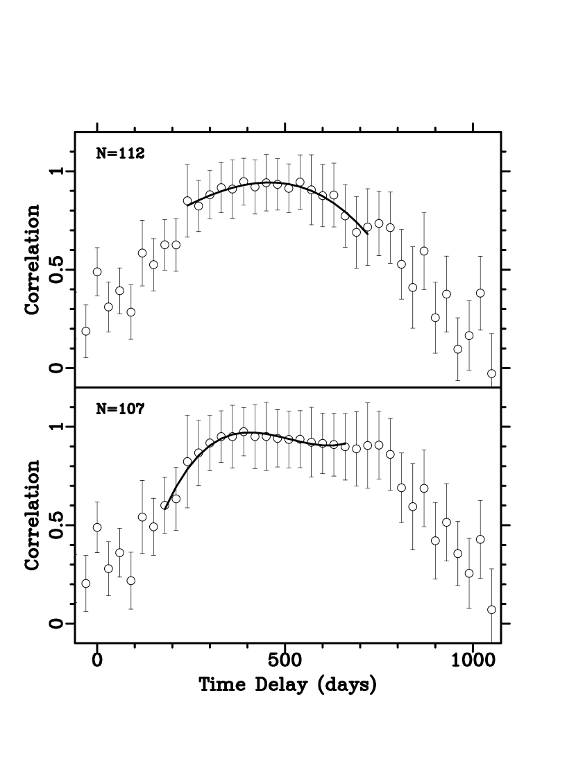
Figure 14: The LNDCF (circles), and the cubic polynomial fit to the peak (thick line), for the N=112 and N=107 light curves.

The LNDCF for the N=112 and N=107 light curves is plotted in Figure 14, showing the LNDCF and its errors for each delay bin, and the cubic fit to the peak of the LNDCF. For N=112, the maximum correlation of 0.943 is at $\tau=458$ days, where about 70 pairs were used in the calculation. The fitted flux ratio for this delay was $R=0.6980$. The 68% confidence intervals and the bias were determined from the 500 N=112 Gaussian Monte Carlo data sets, giving

$$\tau=458^{+27}_{-27}\,{\rm days}, R=0.6982^{+0.0027}_{-0.0026} (N=112,\,{\rm LNDCF}).$$ (27)

For N=107, the maximum correlation of 0.971 was at $\tau=405$ days, where about 60 pairs were used in the calculation. The fitted flux ratio for this delay was $R=0.7000$. Using the 500 N=107 Gaussian Monte Carlo data sets to find the bias and the 68% confidence intervals,

$$\tau=404^{+25}_{-30}\,{\rm days}, R=0.6999^{+0.0030}_{-0.0026} (N=107,\,{\rm LNDCF}).$$ (28)

L92 found a value for the delay of $\tau=513$ (with a correlation of 0.97) when using this method on the first 80 data points. With the addition of the new features in the light curves, the estimate of the delay has shifted to a lower value, in agreement with the PRH$Q$ and dispersion results. Unlike the PRH$Q$ result but in agreement with the dispersion result, the delay estimate is significantly affected by the removal of the five points in Spring 1990. The LNDCF is dominated by the flat portions of the light curve, which swamp out the signal from sharp features, so the removal of the points from the strong 1990 rise make the LNDCF less able to distinguish between delays of interest (note the flatness of the N=107 LNDCF from 350 to 600 days in Figure 14).

We calculated the LNDCF for the N=112 pseudo-jackknife data sets, and found that the delays were scattered between 428 and 489 days (or -30 to +31 days from the delay found above for the real N=112 data), except that removal of 1990 April 10 shifted the delay estimate -44 days to 414 days. The scatter is comparable to the confidence interval obtained from the Gaussian Monte Carlo data. Removal of 1990 April 10 effectively selects the “first rise” in the B image in 1990 (see Section 7). The LNDCF for the N=107 pseudo-jackknife data found delays scattered between 395 and 417 days (-10 to +12 days from the real N=107 data), with the removal of 1989 September 27 shifting the delay estimate -19 days to 386 days. The scatter is smaller than the confidence interval obtained from the Monte Carlo data. Since 1989 September 27 is the last point before the B rise in 1990, it is crucial for alignment with the rise in 1988 of the A image.

7 Discussion and Conclusions

We have calculated time delays by using three different statistical techniques on the complete light curves, and on the light curves with five points removed. Confidence intervals have been found using Gaussian process Monte Carlo data with the same sampling and structure function as the real light curves. Table 3 lists our results. Note that the flux ratio increases with decreasing time delay, a trend that can be seen in the delay-ratio surfaces. Some time delay studies have made the error of assuming one flux ratio while finding the delay, rather than fitting for both parameters at once. The degeneracy between the fitted delay and ratio is probably due to the long decline in the early part of the light curves.

Table 3 contains values ranging from 398 to 461 days. Thus, the new features in the light curves show convincingly that the time delay for the radio light curves is less than 500 days. But which of the delays in Table 3 is correct? We comment here on the advantages and disadvantages of the different statistical methods used.

The PRH$Q$ statistic has the advantage of using all of the data in the light curves ($4N^{2}$ pairs). Each point is compared to every other point, and the difference is checked for consistency with the covariance model, rather than just comparing every point to its nearest neighbors and checking if the difference is zero. The method is less dependent on the exact features of the light curve than the other methods, and instead relies on the statistical properties of the underlying quasar emission and the measurement error. However, PRH$Q$, as applied here, requires two important assumptions about the data: that the light curve is statistically stationary (assumed when we fit one structure function for the whole light curve), and that the covariance model correctly describes the variations in the light curve. Since $Q$ was used to find the covariance model, the second assumption should be a good one. Although the use of $Q$ has reduced the impact of sampling, the gaps in the observations still cause delays of about 480 days to be excluded more strongly than other delays for “window function” data. We confirm the finding of PRHa that the choice of covariance model for the PRH$\chi^{2}$ or $Q$ analysis has little affect on the best fit delay, but find that the choice of covariance model can have a significant affect on the topology of the PRH$\chi^{2}$ surface and the confidence interval found from Monte Carlo analysis.

The dispersion method does not assume that the light curves are stationary, but does assume that nearby points will have identical flux densities if their separation is less than 60 days. The dispersion only uses about 2N pairs of points in the calculation. While the original version of the dispersion given in P94 produced very rough surfaces in time delay, the weighting modifications of P96 have made the dispersion a smooth function of delay and ratio, so that there is a convincing (but broader) global minimum.

The discrete correlation function has the advantage of being completely independent of the flux ratio, since it fits only in delay. It assumes that the light curves are stationary within each delay bin, and assumes that nearby points will have similar flux densities. The number of pairs going into a calculation is on the order of N/2. Because of the bin size, the LNDCF has poor resolution in delay unless it is interpolated at the peak. Furthermore, it is dominated by the non-performing parts of the signal, such as linear ramps and flat sections, rather than the sharper features (thus, non-linear variability is more important for this method than the others).

Given the arguments for and against each method, we are not convinced that one method is superior to the others, and so we are not convinced of a particular value of the time delay. We are convinced that the time delay, based on the current radio light curves, is in the range 375 to 485 days, and definitely less than 500 days. The flux ratio is then in the range 0.695 to 0.707. The large range for the delay has two causes. First, there have been unlucky coincidences of key features in the light curves with gaps in the monitoring (the 1991 B decrease and 1994 A increase), or with unusual variations (the 1990 B increase). Second, although all three methods agree on the time delays inserted in stationary, Gaussian Monte Carlo light curves (with $\sim$5% uncertainty), they disagree by $\sim$15% on the time delay for the real light curves, indicating that the data may have non-Gaussian properties.

Ideally, Monte Carlo data should be made to have all the statistical properties of the real data. The only way to do this with certainty is to derive the Monte Carlo light curves directly from the real ones. P94 and P96 did this by using a bootstrap technique to make Monte Carlo data. They first combined the light curves at their best delay, then applied an adaptive median filter to the combined curves, and finally bootstrapped the residuals. Although they derive the synthetic data from the real data, they also assumed a value for the delay and and assumed that the residuals about the median-filtered light curve are independent and identically distributed (probably not the case). Although our pseudo-jackknife analysis was not formally correct, it was another way to produce synthetic light curves directly from the data. We found that the scatter in the time delay estimates for the pseudo-jackknife data was comparable to, and in some cases better than, the confidence intervals from the Gaussian Monte Carlo light curves. To improve the statistical analysis of the current 6 cm light curves beyond what has been done, the non-Gaussian characteristics of this time series need to be incorporated into the analysis.

The analyses discussed above are statistical, but often one can gain insights into the problem by sliding the curves across one another to get an estimate of the time delay by eye. Figure 15 shows the light curves combined at three delays. When combining the curves, one finds that for longer delays (greater than 500 days), the A image decline around Julian Day 2448000-8500 does not happen soon enough to line up with the B image drop around Julian Day 2448500-2449000. This leads one to expect that the time delay we obtain based on the current light curves will be shorter than the delay obtained previously, which is exactly what we find from the statistical analysis above. Note that at shorter delays (less than 500 days) the fluctuation in the B image in Spring 1990 starts to look out of place. In fact, the B image seems to have two possible rises, either in 1990 February-March or in 1990 May, depending on which points you choose to ignore (see Figure 1). Shorter time delays seem to correspond to assuming the first rise is the real one, the longer time delays seem to correspond to the second rise being real. This explains why the 1990 April 10 and 1990 May 7 B image points are so influential to the time delay analysis, as found by P94. The PRH optimal reconstruction gave us additional information about these points, indicating that the observations in that epoch were produced by a different physical process than the rest of the light curve. Thus we removed the points for both the first and the second rise in Spring 1990 for the N=107 analysis. In the future we may gain a better understanding of the different underlying physical processes, and may be able include those in the model.

Since the A and B light curves show no large differences on time scales of one to fifteen years, we conclude that the VLA 6 cm light curves are not affected by microlensing or other mechanisms on these time scales. This is an advantage of the radio monitoring over optical monitoring projects. However, shorter fluctuations such as that in the B image in Spring 1990 do confuse the analysis. Such variations may be due to microlensing or RISS of a compact jet component emerging from the core of the quasar, and thus would be more likely to occur during times of flux density increase than at other times in the light curve.

An estimate of the time delay, when combined with a mass model, gives us a measurement of the angular diameter distance to the lens. If assumptions are also made about the cosmology, then we can find the Hubble parameter $H_{0}$. While Kochanek (1991) warns against modeling without sufficient observational constraints, others make basic assumptions about the galaxy and cluster in the lens and then do the fit. Falco et al. (1991a) model the galaxy as a King model sphere with a core mass, and the cluster as a shear effect. Grogin & Narayan (1996a, 1996b) model the galaxy as a softened power-law sphere with a core radius, and the cluster as a shear. Grogin & Narayan (1996a, 1996b) fit both of these models to the VLBI observations of Garrett et al. (1994), assuming $\Omega=1$ and $\Lambda=0$. Grogin & Narayan found the fit to the King sphere lens model to have a lower $\chi^{2}$ than the power-law sphere model, although the reduced $\chi^{2}$ of 3.4 was still large, indicating a poor fit to the observational constraints. For the King sphere model they find

$$H_{0}=81.0^{+6.4}_{-6.1}\left(\frac{\sigma}{300\,{\rm km/s}}\right)^{2}\left(\frac{1.1\,{\rm years}}{\tau}\right)\,{\rm km\,s^{-1}Mpc^{-1}}.$$

The velocity dispersion of the galaxy was measured recently by Falco et al. (1996) to be $\sigma=259\pm 10\,{\rm km/s}$ for positions more than 0.2″from the center of the lensing galaxy. Using this velocity dispersion and the shortest delay in Table 3, the King sphere model gives $H_{0}=60.9^{+7.5}_{-7.6}$, while using the longest delay in Table 3 gives $H_{0}=52.6^{+6.1}_{-6.0}$. The quoted uncertainties on these values of $H_{0}$ are one $\sigma$, and 5% error has been added for the ambiguity due to large scale structure along the line of sight (Bar-Kana (1996)).

Continued VLA monitoring of this source will improve our estimate of the delay. The quasar has been more variable in recent years than in the 1980s, and new features may continue to enter the light curve. We have yet to achieve dense sampling of a sharp increase or decrease in both the A and B light curves that is not confused by an unusual variation. Since 1990 October we have been monitoring B0957+561 at 4 cm as well as 6 cm. At the shorter wavelength, the A and B images are resolved in the VLA D array, so the 4 cm light curves will be free of long gaps. The flat-spectrum cores of the A and B images will be better isolated from the extended emission in the image, and the cores should also be more variable. Finally, the multi-wavelength information on the quasar variability will aid in understanding the physical origin of the fluctuations. Joint analysis of the 4 cm and 6 cm light curves will improve our measure of the time delay in the 0957+561 gravitational lens system, and will be reported in a future publication.

Table 1: History of the Time Delay

Reference	Data Set	Statistic	Delay (days)	Delay (years)
Lloyd 1981	28 optical obs	1	$>730$	$>2$
	over 2 years
Keel 1982	17 optical obs	1	$>990$	$>2.7$
	over 2 years
Florentin-Nielsen 1984	54 optical obs	1	$566\pm 40$	$1.55\pm 0.1$
	over 5 years
Bonometti 1985	3 VLBI obs	1	$470\pm 260$	$1.3\pm 0.7$
	over 4 years
Gondhalekar et al. 1986	11 UV obs	1	$660\pm 70$	$1.8\pm 0.2$
	over 4 years
Schild & Cholfin 1986	28 optical obs	3	$376\pm 40$	$1.03\pm 0.1$
	over 4 years
Lehár et al. 1988	40 radio obs	2	$500\pm 100$	$1.4\pm 0.3$
	over 8 years
Vanderriest et al. 1989 (V89)	131 optical obs	3, 4	$415\pm 20$	$1.14\pm 0.05$
	over 8 years
Schild 1990 (S90)	329 optical obs	3	$404$	$1.11$
	over 10 years
Falco, Wambsganss, & Schneider 1991	V89	5	$430\pm 17$	$1.18\pm 0.047$
	S90	5	$490\pm 34$	$1.34\pm 0.093$
Lehár et al. 1992 (L92),	80 radio obs	6	$513\pm 40$	$1.40\pm 0.10$
Roberts et al. 1991	over 11 years
Press et al. 1992a	V89	7	$536^{+14}_{-12}$	$1.47^{+0.038}_{-0.033}$
Press et al. 1992b	L92	7	$548^{+19}_{-16}$	$1.50^{+0.052}_{-0.044}$
	V89, L92	7	$540\pm 12$	$1.48\pm 0.033$
Oknyanskij & Beskin 1993	L92	8	$540\pm 30$	$1.48\pm 0.082$
Pelt et al. 1994	V89, S90	9	$415\pm 32$	$1.14\pm 0.088$
	L92*	9	$409\pm 23$	$1.12\pm 0.063$
Beskin & Oknyanskij 1995	V89, S90	8	$530\pm 15$	$1.45\pm 0.04$
Schild & Thomson 1995 (ST95)	835 optical obs	$\cdots$	$\cdots$	$\cdots$
	over 16 years
Campbell et al. 1995	4 VLBI obs	1	$\sim 365$	$\sim 1$
	over 6 years
Pelt et al. 1996	ST95	10	$423\pm 6$	$1.16\pm 0.016$
	L92*	10	$421\pm 25$	$1.15\pm 0.068$
Kundić et al. 1995, 1996	$\sim$100 optical obs	3, 7, 10	$418.5\pm 6.0$	$1.146\pm 0.016$
	over 2 years
Oscoz et al. 1996, Kundić et al. 1995	40 optical obs	1	$<500$	$<1.4$
	over 1 year
Thomson & Schild 1997	ST95	11	$405\pm 12$	$1.11\pm 0.033$

Note. — Time delays were converted from number given in reference using 1 year = 365.25 days. Statistical techniques are: 1) Inspection, 2) Polynomial Fitting, 3) Interpolation and Cross Correlation, 4) Discrete Fourier Analysis, 5) Dispersion (all pairs), 6) Locally Normalized Discrete Correlation, 7) $\chi^{2}$ Structure Function Analysis, 8) Flux Ratio Dispersion, 9) Dispersion (near-neighbors), 10) Weighted Dispersion (near-neighbors), and 11) Interpolation, Filtering, and Cross Correlation. *1990 April 10 and 1990 May 7 removed

Table 2: VLA 6 cm Light Curve Data

Calendar Date	Observation Array	Julian Day minus 2440000.0	A flux density (mJy)	B flux density (mJy)	Reduction Array
79Jun23	P	4047.50	39.47	31.71	A
79Oct13	P	4160.16	39.26	29.67	A
80Feb23	P	4292.79	37.37	29.69	A
80Jun20	P	4411.30	35.90	29.01	A
80Nov24	A	4567.93	36.04	27.76	A
80Dec16	A	4589.50	35.90	27.50	A
81Jan06	A	4610.99	35.79	27.95	A
81Jan23	A	4628.25	35.64	27.34	A
81Jan24	A	4628.75	35.70	27.09	A
81Jan26	A	4631.47	34.99	27.68	A
81Mar03	A	4666.71	35.10	25.87	A
81Mar27	A	4690.71	35.02	26.65	A
81May14	B	4738.61	34.85	26.59	B
81May28	B	4752.68	35.08	26.89	B
81Jun14	B	4769.55	35.32	26.58	B
81Jul16	B	4802.41	33.86	26.24	B
81Aug15	B	4832.30	34.23	26.34	B
81Oct20	C	4898.16	32.64	26.71	C
81Nov21	C	4930.08	32.22	25.60	C
81Nov25	C	4934.00	32.22	25.10	C
81Dec05	C	4944.06	31.94	24.83	C
82Jan09	C	4978.97	32.36	25.58	C
82Feb09	A	5009.81	33.15	24.73	A
82Mar03	A	5031.75	32.67	25.11	A
82Mar27	A	5055.64	32.40	25.19	A
82May08	A	5097.61	33.48	24.91	A
82Jun03	A	5123.52	32.87	24.68	A
82Jun27	A	5148.41	32.57	24.98	A
82Jul16	B	5167.32	31.81	24.83	B
82Aug21	B	5203.30	31.81	24.48	B
82Sep23	B	5236.13	31.91	23.95	B
82Oct25	B$\rightarrow$D	5268.14	32.73	24.17	B
83Jan20	C	5354.89	31.12	23.18	C
83Feb16	C	5381.81	30.77	23.85	C
83Mar15	C	5408.82	30.61	23.48	C
83Apr03	C	5427.67	32.10	23.76	C
83May05	C	5459.62	31.20	23.08	C
83Aug04	A	5551.41	31.20	23.07	A
83Sep06	A	5584.30	30.52	22.30	A
83Oct08	A	5616.19	30.55	22.75	A
83Nov26	A	5665.06	31.03	22.67	A
84Feb11	B	5741.85	30.94	22.62	B
84Apr22	C	5812.69	30.15	21.51	C
84Jun22	C	5874.43	30.73	22.26	C
84Dec12	A	6046.95	31.82	21.15	A
85Feb12	A	6108.86	32.62	20.64	A
85Apr20	B	6175.72	32.40	21.29	B
85Jun03	B	6219.55	31.16	21.07	B
85Aug17	C	6295.25	30.78	21.11	C
86Feb19	A	6480.80	31.29	22.28	A
86Apr03	A	6523.66	31.40	21.51	A
86May21	A	6571.59	31.98	21.55	A
86Jul20	B	6632.28	30.63	21.53	B
86Sep11	B	6685.12	31.85	22.26	B
86Nov12	C	6747.11	31.44	21.62	C
87Jan11	C	6806.89	31.00	21.62	C
87Jul20	A	6997.35	30.49	20.46	A
87Sep27	A	7066.27	30.99	20.94	A
87Dec09	B	7138.99	31.46	21.79	B
88Jan26	B	7186.83	31.05	21.65	B
88Mar17	C&D	7237.71	30.53	21.77	C
88May08	C&D	7289.59	32.68	22.06	C
88Oct27	A	7462.12	33.26	21.85	A
88Nov18	A	7484.03	35.52	22.35	A
88Dec21	A	7516.98	35.14	21.55	A
89Jan24	A	7550.94	35.12	21.51	A
89Feb24	AnB	7581.75	37.24	22.19	A
89Mar25	B	7610.71	36.47	21.38	B
89Apr26	B	7642.65	37.04	21.11	B
89May19	BnC	7665.56	36.60	21.94	B
89Jun20	C	7697.59	35.52	21.59	C
89Jul16	C	7724.40	38.03	22.51	C
89Sep27	C	7797.28	35.84	21.87	C
90Feb19	A	7941.84	36.49	24.56	A
90Mar15	A	7965.82	36.73	26.14	A
90Apr10	A	7991.65	36.38	22.30	A
90May07	A$\rightarrow$AnB	8018.72	37.09	23.65	A
90May23	A$\rightarrow$AnB	8034.53	34.84	26.63	A
90Jun07	A$\rightarrow$AnB	8049.57	35.35	25.46	A
90Jul15	AnB	8088.36	34.69	25.33	A
90Aug21	B	8125.32	34.75	26.39	B
90Sep06	B	8141.21	35.68	24.75	B
90Oct04	BnC	8169.22	34.04	24.18	B
90Nov01	C	8197.06	32.70	25.35	C
90Dec13	C	8238.89	32.74	25.57	C
91Jan17	C	8273.79	32.40	25.36	C
91Jul10	A	8448.40	31.15	24.81	A
91Aug18	A	8487.31	32.44	25.09	A
92Jan06	B	8627.97	31.32	21.94	B
92Feb04	BnC	8656.80	30.58	23.26	B
92Feb29	C	8681.74	31.13	22.41	C
92Mar07	C	8688.67	31.70	22.57	C
92Apr18	C	8730.60	31.31	22.80	C
92May03	C	8745.60	31.74	22.76	C
92Oct23	A	8919.08	31.15	21.26	A
92Nov11	A	8938.09	31.18	21.92	A
92Dec10	A	8966.97	31.69	21.90	A
93Feb05	AnB	9023.78	30.56	22.73	A
93Mar21	B	9067.64	31.69	22.23	B
93Apr09	B	9086.67	31.40	22.73	B
93Jul25	C	9194.21	30.70	22.58	C
93Aug26	C	9226.26	31.26	22.21	C
94Mar04	A	9415.73	34.50	21.55	A
94Apr11	A	9453.68	34.53	21.03	A
94May07	A$\rightarrow$AnB	9479.63	34.87	21.39	A
94Jun25	B	9528.52	35.58	22.07	B
94Jul06	B	9540.42	34.75	22.56	B
94Aug18	B	9583.28	34.67	22.23	B
94Sep08	B	9604.27	35.42	23.62	B
94Oct10	BnC	9636.18	34.96	21.96	B
94Nov07	C	9664.08	35.37	22.86	C
94Dec08	C	9694.92	34.86	21.58	C

Table 3: Results

Statistic	Light Curve	Time Delay (days)	Flux Ratio
PRH$Q$	N=112	$459^{+14}_{-16}$	$0.6976^{+0.0022}_{-0.0023}$
	N=107	$461^{+16}_{-15}$	$0.6981^{+0.0023}_{-0.0024}$
Dispersion	N=112	$443^{+22}_{-21}$	$0.6995^{+0.0029}_{-0.0030}$
	N=107	$398^{+25}_{-22}$	$0.7039^{+0.0026}_{-0.0030}$
LNDCF	N=112	$458^{+27}_{-27}$	$0.6982^{+0.0027}_{-0.0026}$
	N=107	$404^{+25}_{-30}$	$0.6999^{+0.0030}_{-0.0026}$

Figure 1: The 6 cm light curves of gravitational lens B0957+561, from 1979 to 1994.

Figure 2: Point estimates of the structure function for the N=112 light curves. The crosses are from the A light curve, and the diamonds are from the B light curve. The dotted line is the structure function found by PRHb.

Figure 3: The PRH$\chi^{2}$ surface for N=112 data points, using the PRHb covariance model. The global minimum is PRH$\chi^{2}=283$ at $\tau=455$ days, R = 0.6979, for 221 degrees of freedom. Contours start at PRH$\chi^{2}=285$ and increase by 5 to 430.

Figure 4: Optimal reconstructions for the N=112 light curves, using the PRHb covariance model. The gray region is the one $\sigma$ error about the reconstruction.

Figure 5: Differences between the real data and the optimal reconstruction for the N=112 light curves, using the PRHb covariance model. The gray region is the one $\sigma$ error about the reconstruction. The observed data points and their errors were normalized so that the one $\sigma$ band about the optimal reconstruction was unity. The epoch removed is marked with dashed lines.

Figure 6: Point estimates of the structure function for the N=107 light curves. The crosses are from the A light curve, and the diamonds are from the B light curve. The dotted line is our best fit for the structure function.

Figure 7: The $Q$ surface for N=107 data points, using the new covariance model. The global minimum is $Q=-719$ at $\tau=460$ days and $R=0.6979$. Contours start at $Q=-715$ and increase by five to $Q=-570$.

Figure 8: Optimal reconstructions for the N=107 light curves, using the new covariance model. The gray region is the one $\sigma$ error about the reconstruction.

Figure 9: Differences between the real data and the optimal reconstruction for the N=107 light curves, using the new covariance model. The gray region is the one $\sigma$ error about the reconstruction. The observed data points and their errors were normalized so that the one $\sigma$ band about the optimal reconstruction was unity. The epoch removed is marked with dashed lines.

Figure 10: PRH$Q$ for the N=107 ersatz data (solid line), and for the real N=107 data (dotted line).

Figure 11: The $Q$ surface for N=112 data points, using the new covariance model. The global minimum is $Q=-707$ at $\tau=460$ days and $R=0.6976$. Contours start at $Q=-705$ and increase by five to $Q=-570$.

Figure 12: The dispersion surface for the N=112 light curves. The global minimum is $D^{2}=0.01153$ at $\tau=443$, $R=0.6996$. Contours start at 0.0120 and increase by 0.0005 to 0.0260.

Figure 13: The dispersion surface for the N=107 light curves. The global minimum is $D^{2}=0.00849$ at $\tau=399$, $R=0.7039$. Contours start at 0.0090 and increase by 0.0005 to 0.0230.

Figure 15: Combined light curves. The A light curve is shown with crosses, the B light curve is shown with open circles. The five points removed from A and B are filled squares and circles, respectively. The B light curve has been shifted back by $\tau=405$$\,{\rm days}$ and up by $R=0.700$ (top panel), $\tau=460$$\,{\rm days}$, $R=0.698$ (middle panel), and $\tau=540$$\,{\rm days}$, $R=0.693$ (bottom panel). Error bars have been omitted for clarity. Arrows indicate epochs referred to in the text.

References

- Angonin-Willaime, Soucail, & Vanderriest (1994) Angonin-Willaime, M.-C., Soucail, G., & Vanderriest, C. 1994, A&A, 291, 411
- Bar-Kana (1996) Bar-Kana, R. 1996, ApJ, 468, 17
- Bernstein, Tyson, & Kochanek (1993) Bernstein, G. M., Tyson, J. A., & Kochanek, C. S. 1993, AJ, 105, 816