Evidence for “Chain Reaction” in the
Time Profiles of Gamma Ray Bursts

Abstract

Although the time profiles of gamma ray bursts (GRBs) show extremely diverse behavior, their average statistical properties such as the average peak-aligned profile and the auto-correlation function show simple stretched-exponential behavior. This could indicate that the diversity of all bursts is just due to different random realizations of the same simple stochastic process where the process is scale invariant in time. We illustrate how both the diversity of GRB time profiles and some important average statistical properties can be reproduced in this way using a simple toy model for a stochastic pulse avalanche, which behaves as a chain reaction in a near-critical regime. We suggest that one possibility for the underlying physical process for generating GRBs could be a “chain detonation” in which reconnecting magnetic turbulent features trigger each other.

Stern & Svensson Time Profiles of Gamma Ray Bursts

1 Introduction

The temporal properties of GRBs in the hard X-ray to soft gamma ray band (25 keV - 1000 keV) which are important for our analysis can roughly be summarized as follows:

- The duration of bursts varies by five orders of magnitudes from a few milliseconds to a few hundred seconds and their time profiles are extremely diverse in their complexity and morphology (e.g., [Fishman 1993, Fishman & Meegan 1995]).

- All individual time profiles can probably be considered as a sum of a number of pulses of a more or less standard shape - a sharp rise and a slower exponential decay (for morphologically simple events this is evident, see, e.g., [Norris et al. 1996]). The width of these pulses differs by four orders of magnitude.

- There are very complex events showing a wide range of time scales within a single burst. Many short bursts or short features in long bursts look like rescaled versions of much longer events (e.g., [Norris 1995]). This could indicate multifractality of the time profiles of GRBs (e.g., [Meredith et al. 1995, Yuan Yan et al. 1996]).

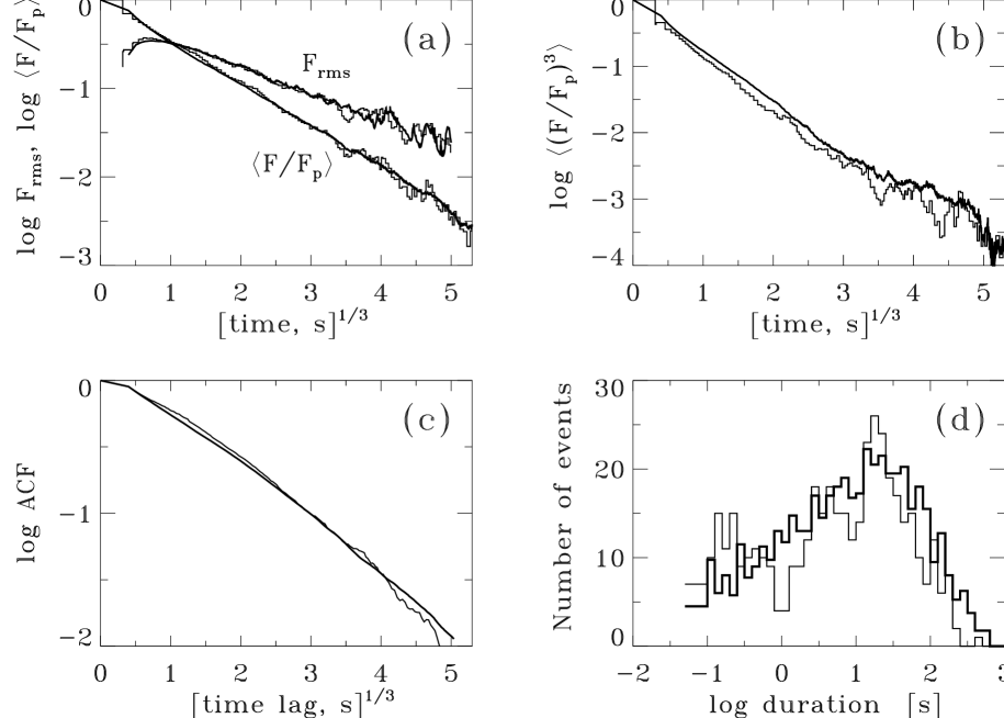
Figure 1: Comparison between observed and simulated average temporal functions of time profiles of GRBs. (a) Thin-line histogram labelled $<F/F_{p}>$ shows the average peak-aligned post-peak time profile for the 598 useful BATSE-3 events as the fractional flux, $<F/F_{p}>$ vs $t^{1/3}$, where $F_{p}$ is the peak flux and $t$ = 0 – 150 s is the time since the strongest peak. Further details are given by Stern (1996). Thick curve labelled $<F/F_{p}>$ is the average peak-aligned time profile for 5000 simulated time profiles. The set of curves labelled $F_{\rm rms}$ are the rms deviations of individual peak-aligned time profiles, $F_{\rm rms}\equiv(<(F/F_{p})^{2}>-<F/F_{p}>^{2})^{1/2}$, for both real (thin line histogram, 598 events) and simulated (thick curve, 5000 events) time profiles. (b) Third moment test, i.e. comparing the peak-aligned $<(F/F_{p})^{3}>$. The only significant difference between the curves is in the relative height of the first bin, representing the peak of the individual time profiles. This is probably due to the effect of Poisson noise which is enhanced here as compared to the first moment profile in (a). (c) Auto-correlation function (ACF) test. The definition of the auto-correlation function for time profiles with Poisson noise are given by Link, Epstein, & Priedhorsky (1993). The average ACF is approximately the same for both real (thin curve, 598 events) and simulated (thick curve, 2000 events) time profiles, except for an excess in the real ACF for time lags 2-10 s (also visible for the average time profile in (a)). The excess may be due to a larger correlation between pulses in real events. (d) Duration distribution test. The number of events of a given duration vs the duration time for both real events (thin line, 432 sufficiently bright events) and simulated events (thick line, 2000 events with the distribution reduced by a factor four). The durations of both real and simulated events were measured at a level of 20 % of the peak amplitude. Real events were filtered to reduce the Poisson noise. For the chosen set of parameters (see text), the positions of the main peak of the simulated and observed duration distributions are in remarkable agreement, while the possible double-humped shape of the observed distribution which has been interpreted as a bimodality of GRBs (Kouveliotou et al. 1993) is not reproduced. A Kolmogorov-Smirnov test shows that these two distributions are drawn from the same parent distribution with a probability of 0.007. The bimodality, if it exists, can be implemented into the model by having the primary pulse width spectrum deviate from $1/f$ flicker noise.

The procedure for obtaining the average peak-aligned time profile of GRBs was pioneered by Mitrofanov et al. (1994, 1995, 1996) (also see Norris et al., 1994, 1996). Stern (1996), studying the average peak-aligned time profile of GRBs in the BATSE-2 catalog, found that the profile has a simple “stretched” exponential shape, $<F/F_{p}>=\exp[-(t/t_{0})^{1/3}]$, where $t$ is the time since the peak flux, $F_{p}$, of the event, and $t_{0}$ is a constant ranging from 0.3 sec for strong bursts to $\sim$ 1 sec for dim bursts. This dependence of $t_{0}$ on brightness could be interpreted as cosmological time dilation (e.g., [Paczyński 1992, Piran 1992]). Here we only consider the average time profile of all GRBs. In Figure 1a, we present the average peak-aligned time profile of GRBs, $<F/F_{p}>$, (thin-line histogram) using the larger statistics of the BATSE-3 catalog. Fitting $<F/F_{p}>=c\exp[-(t/t_{0})^{\nu}]$ where $c$ is an additional parameter, and excluding the first 64 ms bin (likely to be contaminated by Poisson noise) gives $\nu=0.32\pm 0.03$ at the 90 % confidence level. The average time profile does not show any statistically significant deviations from the stretched exponential for over almost 2.5 orders of magnitude in fractional flux, $<F/F_{p}>$, and for three orders of magnitude in time (from 0.1 s to 100 s). Such a simple average time profile is remarkable considering the diverse and chaotic behavior of the individual time profiles of GRBs.

The stretched exponential law is known to describe some characteristics of scale invariant processes associated with fractals, e.g., turbulence ([Jensen, Paladin, & Vulpiani 1992, Ching 1994]). The simple statistical behavior of GRBs could mean that the diversity of all bursts is just due to different random realizations of the same simple stochastic process where the process is scale invariant in time. The stretched exponential time profile for GRBs should not be interpreted as representing some average relaxation process in GRBs, but rather to be a statistical effect reflecting the distributions of pulse widths and time lags between pulses. In this paper, we illustrate how the variety of GRB time profiles can be reproduced using a simple toy model for a pulse avalanche, which behaves as a chain reaction in a near-critical regime. We also obtain satisfactory agreement with a number of the observed temporal statistical properties of GRBs including the stretched exponential shape of the average time profile.

2 A Stochastic Pulse Avalanche Model

Previous attempts with, e.g., shot noise models to model temporal properties have focused on only a few properties such as the power spectra of single bursts ([Belli 1992]), or the average auto-correlation function ([In ’t Zand & Fenimore 1996]). Here, we attempt to interpret the recently discovered stretched exponential as well as several other temporal properties of GRBs by suggesting the following hypothesis:

- All GRBs can be described as different random realizations of the same simply organized stochastic process within narrow ranges of the parameters of the process.

- The stochastic process should be scale invariant in time.

- The stochastic process works near its critical regime. This would explain the large morphological diversity of GRBs.

We also suggest that one possible candidate for the underlying physical process responsible for the stochasticity is magnetohydrodynamic turbulence, where the standard pulses are due to magnetic reconnection events.

It is difficult, if not impossible, because of the peak-aligning procedure to interpret the shape of the time profile using analytical methods. Instead we use numerical methods to develop a simple stochastic toy model that have similar temporal properties as GRBs.

The model we propose is a pulse avalanche, which is a linear Markov process having the following properties:

1.) The elementary event is a pulse with a time constant ($\approx$ pulse width) $\tau$ and a standard shape being parameterized as a Gaussian rise, $A\exp[-(t-t_{p})^{2}/\tau_{r}^{2}]$ for $t<t_{p}$, and an exponential decay, $A\exp[-(t-t_{p})/\tau]$ for $t>t_{p}$, where $t_{p}$ is the time for the peak of the pulse. Fitting of observed pulses gives $\tau_{r}/\tau\sim 0.3-0.5$ (Norris et al. 1996). We use $\tau_{r}/\tau=0.5$. The pulse amplitude, $A$, is sampled from a uniform distribution, $p_{1}(A)=1$, in the range [0, 1].

2.) In a pulse avalanche, each pulse acts as a parent pulse giving rise to a number of baby pulses, $\mu_{b}$, sampled from a Poisson distribution, $p_{2}(\mu_{b})=\mu^{-1}\exp(-\mu_{b}/\mu)$, with the average number being $\mu$. The process is close to its critical runaway regime when $\mu$ is of order unity.

3.) A baby pulse is assumed to be delayed a time, $\Delta t$, with respect to the parent pulse. We parameterize the probability distribution for the Poisson delay as $p_{3}(\Delta t)=(\alpha\tau)^{-1}\exp(-{\Delta t}/{\alpha\tau})$, where $\tau$ is the time constant of the baby pulse, and $\alpha$ is the delay parameter.

4.) How is the time constant of a baby pulse, $\tau$, related to the time constant, $\tau_{1}$, of the parent pulse? Studying individual time profiles we arrive at the intuitive conclusion that $\tau$ and $\tau_{1}$ are of the same order of magnitude and that $\tau<\tau_{1}$ on average. This allows the process to converge even if $\mu$ exceeds 1 as the pulse avalanche eventually reaches an arbitrary short time scale, where a natural frequency cutoff should exist. We parameterize the probability distribution of $\log(\tau/\tau_{1})$ as uniform, $p_{4}[\log(\tau/\tau_{1})]=\mid\delta_{2}-\delta_{1}\mid^{-1}$ , in the range [$\delta_{1}$, $\delta_{2}$], where $\delta_{1}<0,\delta_{2}\geq 0$, and $\mid\delta_{1}\mid>\mid\delta_{2}\mid$.

5.) The process terminates when it converges due to subcritical values of the model parameters.

6.) The start of the pulse avalanche must also be described. We allow for the existence of a number, $\mu_{s}$, of spontaneous primary pulses, sampled from a Poisson distribution, $p_{5}(\mu_{s})=\mu_{0}^{-1}\exp(-\mu_{s}/\mu_{0})$, with the average number of spontaneous pulses per GRB being $\mu_{0}$.

7.) We suggest that the probability distribution of the time constants, $\tau_{0}$, of spontaneous pulses is $p(\tau_{0})\propto 1/\tau_{0}$. This corresponds to flicker noise, i.e. a “$1/f$” spectrum, which is surprisingly wide spread in very different classes of phenomena (e.g., [Press 1978]). Observations imply an upper cutoff, $\tau_{\rm max}$, for $\tau_{0}$. We then sample $\log\tau_{0}$ uniformly between $\tau_{\rm min}$ and $\tau_{\rm max}$, i.e. $p_{6}(\log\tau_{0})=(\log\tau_{\rm max}-\log\tau_{\rm min})^{-1}$, where $\tau_{\rm min}$ should be smaller than the time resolution. Varying $\tau_{\rm max}$ simply rescales all average avalanche properties in time, in this sense, $\tau_{\rm max}$ is a trivial parameter.

8.) The spontaneous primary pulses in a given GRB are all assumed to be delayed with different time intervals, $t$, with respect to a common invisible trigger event. We parameterize the probability distribution for the Poisson delay, $t$, of a given spontaneous pulse as $p_{7}(t)=(\alpha\tau_{0})^{-1}\exp(-{t}/{\alpha\tau_{0}})$, where $\alpha$ is the constant delay parameter used for all pulses (see property 3 above) and $\tau_{0}$ is the time constant of the spontaneous pulse. Each spontaneous pulse gives rise to a pulse avalanche, and it is the overlap of $\mu_{s}$ pulse avalanches that form a GRB. (Alternatively, we could have chosen the spontaneous pulses to appear more or less uniformly over a wider time range that characterizes the evolution time scale of the pulse generating object. The difference between the scenarios appears when the number of spontaneous pulses exceeds unity.)

3 Results of Simulations

The number of model parameters is seven. We found, however, that it is comparatively easy to understand the effects of moving around in parameter space. First, we show how the model works for a certain set of parameters, that was chosen without any serious efforts of optimization: $\mu=1.2$ (chosen by visually examining when model bursts show sufficient complexity), $\alpha=4$ (gives the wanted shape of the average time profile), $\delta_{1}=-0.5$ and $\delta_{2}=0$ (somewhat arbitrary), $\mu_{0}=1$ (arbitrary but reasonable), $\tau_{\rm min}=20$ ms (below the time resolution, 64 ms), $\tau_{\rm max}=26$ s (by finding agreement with the experimental value, $t_{0}=0.82$ s, see Fig. 1a).

Figure 1a tests the shape of the average peak-aligned time profile of the model. The deviations over long time intervals between real and simulated profiles does not exceed 1.5 $\sigma$ and are typically within 1$\sigma$ (where $\sigma=F_{\rm rms}/\sqrt{598}$ is the rms statistical error of the real average time profile for 598 useful BATSE-3 events and where the rms deviation $F_{\rm rms}$ is shown in Fig 1a). This indicates that the two profiles are statistically consistent (an exact quantitative test for statistical consistency is very difficult due to complicated correlations between different parts of the profile). An excellent stretched exponential shape is obtained for $\alpha$ between 3 and 6 and the dependence on other parameters is weak. Outside this interval of $\alpha$, the stretched exponential shape breaks at the level, $<F/F_{p}>\sim 10^{-1.5}$, which would contradict the data. Thus the long stretched exponential behavior is not an intrinsic property of the model, but is achieved for a certain range of the delay parameter $\alpha$. The observed time constant, $t_{0}=0.82$ s, of the average time profile seems to be related to the geometric mean 0.72 s of $\tau_{\rm max}$ and $\tau_{\rm min}$

After the average time profile is fitted by varying only two parameters, $\alpha$ and $\tau_{\rm max}$, we automatically obtain agreement with observed data using a number of other characteristics:

– The root mean square deviations of individual profiles (Fig. 1a). The agreement means that the model not only correctly reproduces the average time profile shape but also the fluctuations of individual profiles.

– The shape of the average peak-aligned distribution of time profiles to the third power (Fig. 1b).

– The average auto-correlation function (ACF), (Fig. 1c). The 2 – 10 s excess of the real ACF over the simulated ACF is statistically significant ($\sim 3\sigma$). The deviation is moderate ($\sim$ 13%), however, and thus the test is reasonably successful.

– The duration distribution (Fig. 1d). Here we claim only approximate agreement as discussed in the figure caption.

In Figure 2, four observed time profiles are compared with simulated time profiles of similar complexity and morphology. Counterparts for each real event were sampled from 300 simulated events using a single set of model parameters fixed to the values given above. The exception is the counterpart for the most erratic event in the BATSE-3 sample (Fig. 2d) where one parameter was changed slightly: the criticality was increased by setting $\delta_{2}$= 0.2 instead of 0.

A visual examination of burst profiles shows that the model is reasonably successful. For a more quantitative comparison, we selected the 325 brightest BATSE-3 bursts and simulated the same number of events using the set of parameter values given above. In order to eliminate brightness selection effects, we wanted the amplitude and background distributions of real and simulated events to be the same. Each simulated event, therefore, had a peak and a background count rate of the $i$-th real event, where $i$ is a random number, $0<i<325$. Furthermore, we imposed Poisson noise at the 64 ms time resolution. Then we made a simple visual morphological classification of both real and simulated bursts using the same criteria. We found 104 real and 91 simulated single peaked events, 43 and 44 double peaked events, 84 and 81 moderately complex events, 94 and 109 erratic events. Repeating the same test for $\mu_{0}=0.5$ instead of $\mu_{0}=1$ gave 112, 46, 79 and 88 simulated events in each class, respectively. Keeping in mind that visual classification is very subjective, especially between moderately complex and erratic events, we note that both results are statistically consistent with the distribution of real bursts. We also note that the actual number of simulated pulses in a GRB often exceeds the visually estimated number.

We still have a number of parameters to use for fine-tuning the model, but obtaining the best fit is beyond the scope of this letter. We just present support for the hypothesis formulated above by using a simple model to demonstrate that a number of temporal properties of GRBs have a natural interpretation in this approach. We cannot and do not claim that we have found the only possible model that satisfy the data, but it is probably the simplest possible one. Such basic features as a $1/f$ spectrum, time lag between pulses as described by property 3) in § 2, and time scaling invariance should probably be present in any model.

The model we present is a version of a chain reaction in a near-critical (slightly subcritical) regime which then naturally provides large fluctuations. One other feature – the $1/f$ spectrum of spontaneous pulses – could also be associated with the near-criticality of the system. This near-criticality could be related to the concept of self-organized criticality that was introduced by Bak, Tang, & Wiesenfeld (1987) in order to explain the widespread occurrence of $1/f$ noise.

4 Discussion

We now discuss the model in terms of the possible underlying physical process. We suggest reconnecting magnetic turbulence as a possible underlying mechanism. Magnetic reconnection can generate abrupt releases of huge amounts of energy into hard X-rays or soft gamma rays. This is the case for solar flares and probably also for AGNs ([Galeev, Rosner, & Vaiana 1979, Haardt, Maraschi, & Ghisellini 1994]). Turbulence is a phenomenon showing spatial and temporal scaling invariance, with the larger scales cascading to smaller scales just as required in our model.

Consider the following illustrative example for a possible scenario for GRBs which incorporates the pulse avalanche. The original trigger event could be the coalescence of two neutron stars (e.g., [Narayan, Paczyński & Piran 1992]) or a catastrophic energy release by a neutron star (e.g., [Usov 1992]). The trigger event itself can be invisible in the BATSE range on the dynamical time scale of the event ([Mészáros & Rees 1993]). Almost all released energy goes into the kinetic energy of the expanding fireball (e.g., [Cavallo & Rees 1978, Paczyński 1990]). Then, at some stage, instabilities develop in the fireball due to interactions with the interstellar medium (e.g., [Rees & Mészáros 1992, Mészáros & Rees 1993]) or due to collisions of blast waves (e.g., [Rees & Mészáros 1994]). Instabilities could lead to the conversion of fireball energy into turbulent magnetic fields and eventually to dissipation through magnetic reconnection.

These reconnection events can proceed as a chain detonation of turbulent features – the reconnection of one feature destabilizes other features each of which will reconnect after some time delay.

The active turbulent phase can last for more than one hundred seconds, but if the probability of spontaneous reconnection is not large ($\mu_{0}\sim 1$), we may see nothing (zero primary pulses), or just one single pulse (the chain is interrupted after the first pulse), or a developed complex avalanche – it all depends on chance. The rest of the fireball energy (probably the major part) dissipates in other directions or on longer time scales and in other energy ranges and is not yet detected.

The scenario described above is just an illustration and for this reason we did not check whether it satisfies necessary temporal and energy requirements. It is, however, probable that the concept of a chain reaction can be built into a number of different scenarios.

There exist more than one hundred models of GRBs ([Nemiroff 1994]). We are not suggesting a new model but rather a new approach to the interpretation of the temporal properties of GRBs, an approach that seems very fruitful and already extends our understanding of time profiles of GRBs.

.6

.6

Figure 2: Observed time profiles of bright GRBs (left panels, count rate vs time after BATSE trigger, trigger # given in panels) and simulated pulse avalanches (right, flux over the maximum amplitude for a single pulse vs time after invisible trigger). The four pairs of time profiles are selected to represent some of the morphological classes discussed in the literature (Fishman 1993, Fishman & Meegan 1995): (a) smooth profile, few peaks, (b) smooth profile, blend of multiple peaks, the simulated event consists of 9 pulses, the real event probably consists of about 10 - 15 pulses, (c) complex profile, well separated episodes of emission, the simulated event consists of 395 pulses, (d) very erratic, chaotic, and spiky bursts, the simulated one consists of 990 pulses, the real one is probably the sum of more than 1000 pulses. The parameters for the three simulations (a)-(c) are the same (see text), For case (d), the criticality is slightly increased by setting $\delta_{2}$ = 0.2 instead of 0. Note that in complex simulated events (as well as in complex real events), the apparent amplitude of spikes is higher in dense pulse bunches as compared to single pulses despite the fact that all simulated pulses have an amplitude sampled uniformly between 0 and 1. The reason is that the high spikes are the unresolved sum of many correlated narrow pulses. The same is probably also the case for real events. The simulations also reproduce observed GRB features such as “flat-top” pulses and sharply terminated events, with the latter being due to avalanche chains converging to very short time scales.