[Detectability of inflation-produced gravitational waves Michael S. Turner

Departments of Physics and Astronomy & Astrophysics, Enrico Fermi Institute, University of Chicago, Chicago, IL 60637-1433
NASA/Fermilab Astrophysics Center, Fermi National Accelerator Laboratory, Batavia, IL 60615-0500

(12 July 1996)

Detection of the gravitational waves excited during inflation as quantum mechanical fluctuations is a key test of inflation and crucial to learning about the specifics of the inflationary model. We discuss the potential of Cosmic Background Radiation (CBR) anisotropy and polarization and of laser interferometers such as LIGO, VIRGO/GEO and LISA to detect these gravity waves.

]

Introduction Inflation addresses most of the fundamental problems in cosmology – the origin of the flatness, large-scale smoothness, and small density inhomogeneities needed to seed all the structure seen in the Universe today. If correct, it would extend our understanding of the Universe to as early as $10^{-32}\sec$ and open a window on physics at energies of order $10^{15}\,$GeV. However, at the moment there is little evidence to confirm or to contradict inflation and no standard model of inflation.

The key to testing inflation is to focus on its three basic predictions [1]: spatially flat Universe (total energy density equal to the critical energy density); almost scale-invariant spectrum of gaussian density perturbations [2]; and almost scale-invariant spectrum of stochastic gravitational waves [3]. The first two predictions have important implications: the existence of nonbaryonic dark matter, as big-bang nucleosynthesis precludes baryons from contribution more than about 10% of the critical density [4], and the cold dark matter scenario for structure formation, based upon the idea that the nonbaryonic dark matter is slowly moving elementary particles left over from the earliest moments [5, 6]. A host of cosmological observations are now beginning to sharply test the first two predictions [6].

Gravity waves are a telling test and probe of inflation: They provide a consistency check (see below); they are essential to learning about the scalar potential that drives inflation [7]; and they are a compelling signature of inflation – both a flat Universe and scale-invariant density perturbations were advocated before inflation.

Detecting inflation-produced gravity waves presents a great experimental challenge [8]. In this Letter we discuss the potential of CBR anisotropy or polarization and of direct detection by the laser-interferometers to test this key prediction of inflation.

Quantum Fluctuations The (Fourier) spectra of metric fluctuations excited during inflation are characterized by power laws in wavenumber $k$, $k^{n}$ for density perturbations (scalar metric fluctuations) and $k^{n_{T}-3}$ for gravity waves (tensor metric fluctuations). Scale invariance for density perturbations ($n=1$) corresponds to fluctuations in the Newtonian potential that are independent of wavenumber; scale invariance for gravity waves ($n_{T}=0$) corresponds to dimensionless horizon-crossing strain amplitudes that are independent of wavenumber. The power-law indices are related to the scalar field potential, $V(\phi)$, that drives inflation:

$$n-1 = -{m_{\rm Pl}^{2}\over 8\pi}\left({V_{*}^{\prime}\over V_{*}}\right)^{2}+{m_{\rm Pl}^{2}\over 4\pi}\left({V_{*}^{\prime}\over V_{*}}\right)^{\prime},$$ (1)

$$n_{T} = -{m_{\rm Pl}^{2}\over 8\pi}\left({V_{*}^{\prime}\over V_{*}}\right)^{2}.$$ (2)

The overall amplitude of each spectrum can be characterized by its contribution to the quadrupole anisotropy of the CBR,

$$S\equiv{5\langle|a^{S}_{2m}|^{2}\rangle\over 4\pi} = {2.2(V_{*}/m_{\rm Pl}^{4})\over(m_{\rm Pl}V_{*}^{\prime}/V_{*})^{2}},$$ (3)

$$T\equiv{5\langle|a^{T}_{2m}|^{2}\rangle\over 4\pi} = 0.61(V_{*}/m_{\rm Pl}^{4}),$$ (4)

where $S$ refers to scalar and $T$ to tensor, $V_{*}$ is the value of the inflationary potential when the present horizon scale ($k=H_{0}$) crossed outside the Hubble radius during inflation, $V_{*}^{\prime}$ is the first derivative of the potential at that point, and $m_{\rm Pl}=1.22\times 10^{19}\,$GeV [9].

There is a very important relation between amplitude ($T/S$) and tilt ($n_{T}$), cf. Eqs. (1-4),

$$n_{T}=-{1\over 7}\,{T\over S}.$$ (5)

It not only provides a consistency check of inflation [10], but it also has implications for the direct detection of gravity waves, as it relates the overall amplitude to the tilt. Note too, that the tensor amplitude $T$ determines the value of the inflationary potential, and together with $T/S$ and $n$, the first two derivatives of the potential. Any attempt to reconstruct the inflationary potential requires knowledge of the gravity-wave spectrum [7].

FIG. 1.: Angular power spectra ($C_{l}\equiv\langle|a_{lm}|^{2}\rangle$) of CBR anisotropy for gravity waves (lower curves) and density perturbations (upper curves), normalized to the quadrupole anisotropy; broken lines indicate sampling variance. Temperature fluctuations measured on angular scale $\theta$ are approximately, $(\delta T/T)_{\theta}\sim\sqrt{l(l+1)C_{l}/2\pi}$ with $l\sim 200^{\circ}/\theta$ (courtesy of M. White and U. Seljak).

CBR Inflation-produced density fluctuations and gravity waves each give rise to CBR anisotropy and polarization, specified by their predictions for the variance of the multipole amplitudes of anisotropy and polarization [11]. The CBR signatures are very different: the tensor angular power spectrum falls off quickly for $l>100$ and its level of polarization is about 30 times greater for $l<30$ (see Figs. 1 and 2). However, there is a fundamental limit to the accuracy with which the variance of the multipoles can be determined: Because only $2l+1$ multiple amplitudes can be measured for a given $l$, the variance can be estimated to a relative precision of $1/\sqrt{l+{1/2}}$ (known as sampling, or cosmic, variance).

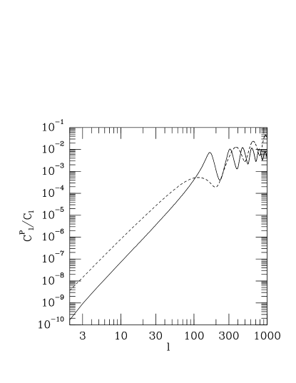
FIG. 2.: Polarization angular power spectra for gravity waves (broken) and density perturbations (solid). The polarization of the CBR anisotropy is roughly $\sqrt{C_{l}^{P}/C_{l}}$ (courtesy of M. White and U. Seljak).

Due to sampling variance $T/S$ must be greater than about 0.1 to ensure that the tensor signature of CBR anisotropy can be detected [12]. In principle, polarization is more promising – $T/S$ as small as 0.02 could be detected [12]. In practice, approaching this limit would be extremely difficult, requiring the polarization of the anisotropy to be measured with 0.01% precision on large-angular scales. Further, the polarization on these scales is very sensitive to the ionization history of the Universe.

FIG. 3.: Spectral energy density in gravity waves produced by inflation; for $T/S=0.018$, $dn_{T}/d\ln k=-10^{-3}$, 0, $10^{-3}$. $T/S=0.18$ (heavy curve) maximizes the energy density at $f=10^{-4}\,$Hz. Curves are from Eq. (6) using $H_{0}=60{\rm km\,s^{-1}\,Mpc^{-1}}$, $\Omega_{0}=1$, and $g_{*}=3.36$.

Direct Detection The inflation-produced background of gravity waves offers at least one advantage – the energy per logarithmic frequency interval is roughly constant for $f=10^{-15}\,$Hz to $10^{15}\,$Hz (see Fig. 3),

$${d\Omega_{\rm GW}\over d\ln k}={\Omega_{0}^{2}\,(V_{*}/m_{\rm Pl}^{4})\,\over(k/H_{0})^{2-n_{T}}}\left[1+{4\over 3}{k\over k_{\rm EQ}}+{5\over 2}\left({k\over k_{\rm EQ}}\right)^{2}\right],$$ (6)

where $k_{\rm EQ}=6.22\times 10^{-2}\,{\rm Mpc^{-1}}\,(\Omega_{0}h^{2}/\sqrt{g_{*}/3.36})$, is the scale that entered the horizon at matter-radiation equality, $\Omega_{0}$ is the fraction of critical density in matter (the balance of critical density is assumed to be in vacuum energy), $\Omega_{\rm GW}$ is the fraction of critical density in gravity waves, wavenumber $k=2\pi f$, the Hubble constant $H_{0}=100h\,{\rm km\,s^{-1}\,Mpc^{-1}}$, and $g_{*}$ counts the effective number of relativistic degrees of freedom (3.36 for the CBR and three massless neutrino species). The factor in square brackets in Eq. (6) is a numerical fit to the transfer function for gravitational waves, which accounts for the evolution of gravity-wave modes after they re-enter the horizon (see Ref. [13] for details).

The relationship between the tensor spectral index and the overall amplitude can be used to rewrite Eq. (6) in terms of $n_{T}$ (or $T/S$) alone. Using the fact that the variance of the CBR quadrupole is given by the sum of the scalar and tensor contributions ($Q=T+S$) and the COBE measurement, $Q\simeq 4.4\times 10^{-11}$ [14], it follows that on the “long plateau” ($k\gg k_{\rm EQ}$, $f\gg 10^{-15}\,$Hz)

$${d\Omega_{\rm GW}h^{2}\over d\ln k} = 5.1\times 10^{-15}\,(g_{*}/3.36)\,{n_{T}\over n_{T}-1/7}$$ (7)

$$\times \exp[n_{T}N+{1\over 2}N^{2}(dn_{T}/d\ln k)],$$ (8)

where $N\equiv\ln(k/H_{0})\simeq 33+\ln(f/10^{-4}{\rm Hz})+\ln(0.6/h)$. Note, if there are additional seas of relativistic particles beyond the photons and three neutrino species ($g_{*}>3.36$), as has been advocated to improve the agreement between the cold dark matter scenario and observations of large-scale structure [15], the energy density in gravity waves is increased, perhaps by a factor of three [16].

FIG. 4.: The range of $T/S$ probed (interval interior to parabola) as a function of energy sensitivity for $f=10^{-4}\,$Hz (solid curves) and $f=100\,$Hz (broken curves). The “pessimistic” (left) parabola assumes $dn_{T}/d\ln k=-10^{-3}$ and the “optimistic” (right) parabola assumes $dn_{T}/d\ln k=10^{-3}$. Also shown are the limiting sensitivity of CBR anisotropy and polarization.

Since the spectrum is normalized at the Hubble scale ($k=H_{0}$) and extrapolated to frequencies that are some 15 orders of magnitude larger we have included the first correction for the variation of the power-law index with scale. The “running” of $n_{T}$ is given by [17],

$${dn_{T}\over d\ln k}=-n_{T}[(n-1)-n_{T}]=-n_{T}\,{m_{\rm Pl}^{2}\over 4\pi}\left({V_{*}^{\prime}\over V_{*}}\right)^{\prime}.$$ (9)

Typically, $dn_{T}/d\ln k\approx-10^{-3}$ [17]; it can be of either sign or even zero [18]. On a very optimistic note, a CBR determination of $T/S$ and a laser interferometric determination of the average spectral index (${\bar{n}_{T}}=n_{T}+0.5Ndn_{T}/d\ln k$) would allow the inference of $dn_{T}/d\ln k$.

An important feature of Eq. (7) is the amplitude – tilt relationship: $n_{T}$ increases the prefactor, but tilts the spectrum so as to decrease the amplitude at high frequencies. At fixed frequency, the energy density is maximized for $n_{T}=-\left(\sqrt{1+28/N}-1\right)/14\approx-0.025$ ($f=10^{-4}\,$Hz). Values for $n_{T}$ of this order are realized in several models of inflation, e.g., chaotic inflation.

The energy density in a stochastic background of gravitational waves can be expressed in terms of the rms strain, $h_{rms}^{2}(k)\equiv k^{3}|h_{\bf k}|^{2}/2\pi^{2}$,

$${d\Omega_{\rm GW}\over d\ln k} = {2\pi^{2}\over 3}\,\left({f\over H_{0}}\right)^{2}\,h_{rms}^{2}(k)$$ (10)

$$= 6.3h^{-2}\times 10^{-7}\,(f/{\rm Hz})^{2}\,(h_{rms}/10^{-21})^{2}.$$ (11)

For fixed strain sensitivity, the energy-density sensitivity varies with the square of the frequency because $\rho_{\rm GW}\propto h_{rms}^{2}f^{2}$, and so prospects for detection improve as $1/f^{2}$.

The range of $T/S$ accessible to a gravity-wave detector operating at $f=10^{-4}\,$Hz and $f=100\,$Hz is shown as a function of energy sensitivity in Fig. 4. For either frequency, a sensitivity of $d\Omega_{\rm GW}h^{2}/d\ln k\sim 10^{-15}$ is needed for a serious search for inflation-produced gravity waves. (The curves in Fig. 4 were computed from Eq. (7) with $\Omega_{0}=1$ and $g_{*}=3.36$; for $\Omega_{0}<1$, only the labeling of the ordinate changes, as the relation $T/S=-7n_{T}$, used to obtain the $T/S$ values, is modified slightly [19].)

LIGO and the other detectors now being built will operate at frequencies from 10 Hz to several kHz, with initial strain sensitivities of around $10^{-21}$, improving to $10^{-24}$ (at $f=10^{2}\,$Hz) [20]. Eq. (7) tells the sad story: Even the most optimistic estimate for LIGO’s energy sensitivity misses the mark by four orders of magnitude. While Earth-based detectors cannot operate at lower frequencies because of seismic noise, space-based detectors can. Early estimates indicated that a strain sensitivity of slightly better than $h_{rms}=10^{-21}$ might be achieved at a frequency of $10^{-4}\,$Hz [21], implying an energy sensitivity $d\Omega_{\rm GW}/d\ln k\sim 10^{-16}$, sufficient to probe $T/S\sim 0.01$. However, the design study for LISA indicates an energy sensitivity of around $d\Omega_{\rm GW}h^{2}/d\ln k\sim 10^{-13}$, which misses by two orders of magnitude [22]. (There is also a worrisome background of coalescing white-dwarf binaries, which could dominate inflation at frequencies greater than around $10^{-4}\,$Hz [21].)

Summary Gravity waves are an important prediction of inflation. The CBR is sensitive to the longest-wavelength gravity waves ($10^{26}\,$cm to $10^{28}\,$cm), but is fundamentally limited by sampling variance. The high-resolution ($l=2-2000$) anisotropy maps that will be made by two future satellite experiments, MAP and COBRAS/SAMBA, might reach the sampling-variance limit, $T/S\sim 0.1$. Improving this by polarization measurements does not look promising. Laser interferometers are sensitive to much shorter wavelengths ($10^{8}\,$cm to $10^{13}\,$cm). An energy sensitivity $d\Omega_{\rm GW}h^{2}/d\ln k\sim 10^{-15}$ is required to search for the inflation-produced gravity-wave background; a sensitivity of $10^{-16}$ opens the window wide, perhaps allowing $T/S$ smaller than $0.01$ to be detected. While Earth-based laser interferometers are not likely to achieve this, there is some hope that space-based detectors operating at low frequencies ($<10^{-4}\,$Hz) might.

We should temper our conclusions, which are based upon the most accurate predictions available, with acknowledgment of their limitations and our possible ignorance. Assumptions have been made: one-field, slow-rollover inflation with a smooth potential. Nature could be more interesting. If inflation ends with the nucleation of bubbles there is an additional potent source ($\Omega_{\rm GW}\sim 10^{-6}$) of gravitational waves in a narrow frequency range [23]; pre-big-bang models predict a spectrum of gravity waves that rises with frequency, making detection far more promising [24]; Grishchuk [25] has long emphasized the production of gravitational waves during the earliest moments in a variety of scenarios. Even if a sensitivity of $d\Omega_{\rm GW}h^{2}/d\ln k\sim 10^{-15}$ cannot be achieved, it is still worth searching – there could be surprises!

We thank M. White for useful discussions. This work was supported by the DoE (at Chicago and Fermilab) and by the NASA (at Fermilab by grant NAG 5-2788).

REFERENCES

- [1] See e.g., E.W. Kolb and M.S. Turner, The Early Universe (Addison-Wesley, Redwood City, CA, 1990), Ch. 8. Not all agree that is a robust prediction of inflation; see e.g., M. Bucher A.S. Goldhaber, and N. Turok, Phys. Rev. D 52, 3314 (1995); J.R. Gott, Nature 295, 304 (1992).
- [2] A. H. Guth and S.-Y. Pi, Phys. Rev. Lett. 49, 1110 (1982); S. W. Hawking, Phys. Lett. B 115, 295 (1982); A. A. Starobinskii, ibid 117, 175 (1982); J. M. Bardeen, P. J. Steinhardt, and M. S. Turner, Phys. Rev. D 28, 697 (1983).
- [3] V.A. Rubakov, M. Sazhin, and A. Veryaskin, Phys. Lett. B 115, 189 (1982); R. Fabbri and M. Pollock, ibid 125, 445 (1983); A.A. Starobinskii, Sov. Astron. Lett. 9, 302 (1983).
- [4] See e.g., C.J. Copi, D.N. Schramm and M.S. Turner, Science 267, 192 (1995).
- [5] See e.g., G. Blumenthal et al., Nature 311, 517 (1984)
- [6] S. Dodelson, E. Gates and M.S. Turner, astro-ph/9603081.
- [7] E.J. Copeland, E.W. Kolb, A.R. Liddle, and J.E. Lidsey, Phys. Rev. Lett. 71, 219 (1993); Phys. Rev. D 48, 2529 (1993); M.S. Turner, ibid, 3502 (1993); ibid 48, 5539 (1993).
- [8] One opinion has it that inflation-produced gravity waves are undetectably small in any reasonable model of inflation (D. Lyth, hep-ph/9606387).
- [9] All formulae are given to lowest order in the deviation from scale invariance and are strictly applicable to single-field models with smooth potentials; see A.R. Liddle and M.S. Turner, Phys. Rev. D 50, 758 (1994).
- [10] R. Davis et al., Phys. Rev. Lett. 69, 1856 (1992); F. Lucchin, S. Mattarese, and S. Mollerach, Astrophys. J. 401, L49 (1992); D. Salopek, Phys. Rev. Lett. 69, 3602 (1992); A. Liddle and D. Lyth, Phys. Lett. B 291, 391 (1992); J.E. Lidsey and P. Coles, Mon. Not. R. astron. Soc. 258, 57p (1992); T. Souradeep and V. Sahni, Mod. Phys. Lett. A 7, 3541 (1992).
- [11] Isotropy in the mean implies that ; the gaussian nature of the inflationary metric fluctuations implies that the multipole amplitudes have gaussian distributions, fully specified by their predicted variances.
- [12] L. Knox and M.S. Turner, Phys. Rev. Lett. 73, 3347 (1994).
- [13] M.S. Turner, J.E. Lidsey and M. White, Phys. Rev. D 48, 4613 (1993).
- [14] K. Gorski et al., Astrophys. J., in press (1996). The normalization depends upon both and ; for the accuracy needed here, this complication can be ignored.
- [15] S. Dodelson, G. Gyuk, and M.S. Turner, Phys. Rev. Lett 72, 3578 (1994); J.R. Bond and G. Efstathiou, Phys. Lett. B 265, 245 (1991).
- [16] This is simple to understand: the drop in energy density from the Hubble scale to the plateau is given by the redshift of matter – radiation equality, which is inversely proportional to the energy density in radiation.
- [17] A. Kosowsky and M.S. Turner, Phys. Rev. D 52, R1739 (1995).
- [18] Given the inflationary potential the gravity-wave spectrum can be computed without assuming a power law; we have done this for chaotic inflation models, , to judge the accuracy of our approximation. It is typically better than 33%. In addition, since there is no standard model of inflation, the use of and to extrapolate the gravity-wave spectrum from very large scales offers the advantage of generality.
- [19] M.S. Turner and M. White, Phys. Rev. D 53, 6822 (1996).
- [20] See e.g., A. Abramovici et al., Science 256, 325 (1992) and in Particle and Nuclear Astrophysics and Cosmology in the Next Millennium, eds. E.W. Kolb and R.D. Peccei (World Scientific, Singapore, 1995), p. 398;N. Christensen, Phys. Rev. D 46, 5250 (1992); B. Allen, qr-gc/9604033.
- [21] K.S. Thorne, in 300 Years of Gravitation, eds. S.W. Hawking and W. Israel (Cambridge Univ. Press, Cambridge, 1987), p.330.
- [22] Pre-phase A Design Study for LISA.
- [23] A. Kosowsky, M.S. Turner, and R. Watkins, Phys. Rev. Lett. 69, 2026 (1992).
- [24] R. Brustein, M. Gasperini, M. Giovannini, and G. Veneziano, Phys. Lett. B 361, 45 (1995).
- [25] S.P. Grishchuk, Zh. Eksp. Teor. Fiz. 67, 825 (1974) [Sov. Phys. JETP 40, 409 (1975)].