AGAPE: a search for dark matter towards M 31 by microlensing effects on unresolved stars

Abstract

M 31 is a very tempting target for a microlensing search of compact objects in galactic haloes. It is the nearest large galaxy, it probably has its own dark halo, and its tilted position with respect to the line of sight provides an unmistakable signature of microlensing. However most stars of M 31 are not resolved and one has to use the “pixel method”: monitor the pixels of the image rather than the stars. AGAPE is the implementation of this idea. Data have been collected and treated during two autumns of observation at the 2 metre telescope of Pic du Midi. The process of geometric and photometric alignment, which must be performed before constructing pixel light curves, is described. Seeing variations are minimised by working with large super-pixels ($2.1\arcsec$) compared with the average seeing. A high level of stability of pixel fluxes, crucial to the approach, is reached. Fluctuations of super-pixels do not exceed 1.7 times the photon noise which is 0.1% of the intensity for the brightest ones. With such stable data, 10 microlensing events are expected for a full “standard halo”. With a larger field, a regular and short time sampling and a long lever arm in time, the pixel method will be a very efficient tool to explore the halo of M 31.

1 The background of the AGAPE search

1.1 Dark matter in galaxies

The presence of a large amount of unseen matter is a very old astrophysical problem (Oort [1932], Zwicky [1933]) but its importance was widely recognised only in the seventies (Ostriker, Peebles & Yahil [1974], Faber & Gallagher [1979]). Actually there are several “dark matter problems” on different scales: stellar systems, individual galaxies, clusters and superclusters of galaxies, up to cosmological scales. Dark matter appears also necessary to understand large structures formation. For a recent review on these subjects, see Dolgov ([1995]). Many observations suggest that spiral galaxies are embedded in massive dark haloes (Kormandy & Knapp [1987], Trimble [1987]). The most conspicuous evidence for such haloes is the rotation curve of galactic disks, which does not decrease near the outskirts of galaxies. If the mass density and surface brightness profiles were similar, the rotation curve should fall according to Kepler’s law.

From the rotation curves of spiral galaxies, one can estimate the amount of dark matter within 2 Holmberg radii to be larger by one order of magnitude than the amount of luminous matter, but the shape of dark haloes is unknown. Several lines of argument point towards a more or less spherical distribution, such as the existence of galaxies with a rapidly rotating polar ring, the stability of the disk of spiral galaxies against bar formation (Ostriker & Peebles [1973]) or the distribution of the globular clusters (Harris & Racine [1979]). The sphere seems often flattened in the direction of the rotation axis (for a recent review, see Sackett [1995] and references therein).

The nature of dark haloes remains also unknown. Many candidates have been proposed, either baryonic or not, ranging from light neutrinos to very heavy black holes of 10${}^{6}\;M_{\odot}$, but it is out of the scope of this paper to review them extensively (for recent reviews, see for instance Dolgov [1995] and Griest [1995]) . Nevertheless, we can mention some unconventional views, such as the modified Newton dynamics (Bekenstein & Milgrom [1984]), or cold molecular hydrogen as the constituent of dark haloes of spiral galaxies (Pfenniger, Combes & Martinet [1994]).

1.2 Baryonic dark matter

Although the subject of primordial abundances has recently become rather confused, Big Bang Nucleosynthesis indicates that the density of baryonic matter in the universe is probably around 10 times larger than that seen as stars or interstellar gas (for a recent discussion, see for instance Cardall & Fuller [1996] and references therein). But the Cosmological Standard Model gives no hint as to the location of this baryonic matter and its relative distribution between galactic haloes and intergalactic medium in clusters of galaxies.

It has been suggested that galactic dark matter could be essentially made of compact baryonic objects such as low mass stars or brown dwarfs. Brown dwarfs are stars too light ($M<0.08M_{\odot}$) for the gravitational pressure to fire nuclear reactions and are a natural candidate for the constituent of galactic haloes (Carr, Bond & Arnett [1984]). It is considered that they should be heavier than 10${}^{-7}M_{\odot}$ lest they would evaporate too quickly (De Rújula, Jetzer & Massó [1992]). Such objects should most easily be seen in the red and infrared bands (Kerins & Carr [1991]). A few may have been in fact observed, some orbiting brighter compagnons: GD 165B (Zuckerman & Becklin [1988]) and Gl229B (Nakajima et al. [1995], Allard et al. [1996]), as well as others free flying in the Pleiades cluster: PPl 15 (Stauffer, Hamilton & Probst [1994]), Teide 1 (Rebolo, Zapaterio Osorio & Martín [1995]) and Calar 3 (Zapaterio Osorio, Rebolo & Martín [1996]). Both PPl 15 and Teide 1 have residual Lithium, and Calar 3 resembles Teide 1 like a twin. (Basri, Marcy & Graham [1996], Martín, Rebolo & Zapaterio Osorio [1996]).

1.3 Gravitational microlensing

Direct searches for brown dwarfs can at best explore the solar neighbourhood. To detect them further out, it was proposed a few years ago by Paczyński ([1986]) to search for dark objects through gravitational lensing. When a compact object passes near the line of sight of a background star, the luminosity of this star will be temporarily increased in a characteristic way.

Several experiments have been implementing this idea since 1990 and have indeed seen microlensing events. Two groups have been looking towards the Magellanic Clouds: the EROS collaboration (Aubourg et al. [1993], Ansari et al. [1995a], Milsztajn [1996]) and the MACHO collaboration (Alcock et al. [1993, 1995a], Bennett [1996]). Microlensings have also been searched for in the direction of the galactic bulge by three groups: OGLE (Udalski et al. [1993, 1994]), MACHO (Alcock et al. [1995b], Sutherland [1996]) and DUO (Alard, Mao & Guibert [1995], Alard [1996]), who have observed a large number of events. The microlensing phenomenon can now be considered as established.

However, the number of events towards the Large Magellanic Cloud (LMC) is lower than expected, 50% or less of what one would expect with a standard spherical halo (Bennett [1996], Milsztajn [1996]), but statistics remain very poor. Moreover, with only one line of sight, it is very difficult to disentangle the various parameters which enter in a galactic halo model: density, velocity distribution, mass distribution, flattening.

MACHO will continue for two more years and the upgrade of EROS (Couchot [1996]) will start operation soon. However, the “classical” technique used in these experiments does not allow to explore other directions through the halo, because the two Magellanic Clouds are the only possible targets with enough resolved stars.

1.4 Going further, the “pixel method”

It is thus tempting to look at rich fields of stars further out, such as the M 31 galaxy. But most stars of M 31 are not resolved and a new technique must be developed. Such a technique, the “pixel method”, has been proposed and implemented by us (Baillon et al. [1992, 1993], Ansari et al. [1995b]). A similar idea, relying on image subtraction, has been independantly proposed by (Crotts [1992]), and implemented by the Columbia-VATT collaboration (Tomaney & Crotts [1994], Tomaney [1996]).

The method we propose is the following: in a dense field of stars, many of them contribute to each pixel. However if one unresolved star is sufficiently magnified, the increase of the total flux of the pixel will be large enough to be detected. Therefore, instead of monitoring individual stars, we propose to follow the luminous intensity of the pixels of the image. Then all stars in the field, and not the only few resolved ones, are candidates for a micro-lensing, so that the event rate is potentially much larger. Of course, only the brightest stars will be amplified enough to become detectable above the fluctuations of the background, unless the amplification is very high and this occurs very seldom. In a galaxy like M 31, however, this is compensated for by the very high density of stars, and indeed various evaluations (Baillon et al. [1993], Jetzer [1994], Colley [1995], Han & Gould [1996]) show that a fair number of events should be detectable.

This paper is devoted to the description of AGAPE (Andromeda Gravitational Amplification Pixel Experiment), which implements this idea in the direction of M 31, on data taken in autumns 1994 and 1995 at the 2 metre telescope Bernard Lyot (TBL) at Pic du Midi Observatory in the French Pyrénées.

In section 2, after recalling the principles of the method, (introduced in Baillon et al. [1992] and [1993]), we give analytic evaluations of the number of events expected. Although these analytic estimates can at best be very rough, they provide useful qualitative insights. To get reliable estimates in the true observational conditions, we resort to Monte-Carlo simulations.

In section 3 we describe the telescope, the detector, the conditions and the course of the observations. Section 4 is devoted to the geometric and photometric alignments of successive images and to the absolute photometry. In section 5 we show that the high level of stability reached on the average super-pixel (a group of $7\times 7$ elementary pixels) allows us to detect variable objects that would have been very difficult to see otherwise. The detailed analysis of the variations we detect will be the subject of separate publications.

The pixel method should also give interesting results in the bar of the LMC, and we have started to analyse the data of the EROS collaboration in this framework (Melchior [1995]). The results will also be published elsewhere.

2 The pixel method

The photon flux of an individual star, $F_{\mathrm{star}}$, is spread among all pixels of the seeing disk and only part of this light, the seeing fraction $f$, reaches the pixel nearest to the centre of the star:

$$F_{\mathrm{star,\;pixel}}=f\times\ F_{\mathrm{star}}.$$ (1)

In a crowded field such as M 31, the light flux $F_{\mathrm{pixel}}$ on a pixel comes from the many stars in and around it, plus the sky background.

$$F_{\mathrm{pixel}}=F_{\mathrm{neighbouring\ stars}}+F_{\mathrm{skybackground}}$$ (2)

If the luminosity of a particular star is amplified by a factor $A$, the pixel flux increases by:

$$\Delta F_{\mathrm{pixel}}=(A-1)\ f\ F_{\mathrm{star}}\,.$$ (3)

The amplification of the star luminosity can be detected if the flux on the pixel nearest to its centre rises sufficiently high above the rms fluctuation $\sigma_{\mathrm{pixel}}$:

$$\Delta F_{\mathrm{pixel}}>Q\ \sigma_{\mathrm{pixel}}\,.$$ (4)

Of course, to be detected, a lensing event should be visible on several exposures. One therefore typically requires that condition (4) be verified for at least 3 consecutive pictures with $Q=3$ and with $Q=5$ for at least one of the three.

Seeing variations induce unwanted fluctuations of the pixel fluxes. To minimise this problem, and to collect most of the light of any varying object, we replace each elementary pixel by a “super-pixel” centered on it. Each super-pixel is a square of $n\times n$ elementary pixels. The size of the square is chosen large enough to cover the whole seeing disk in most cases, but also not too large, to avoid dilution of a variable signal when it occurs. We have also tried to replace each pixel by an average of the neighbouring pixels weighted with the point spread function (PSF), as it is known to maximize the signal to noise ratio at the center of a star on a given image. However, for this very reason, it turns out that this procedure amplifies considerably the fluctuations in time due to seeing variations and therefore it is not appropriate for our method.

2.1 Microlensing tests

All of the classical tests can be applied to discriminate microlensing events against other sources of light variations.

Uniqueness

The probability of a microlensing occurring twice on stars contributing to the same pixel is very weak, and it is safe to reject all non unique events.

Symmetry

Except in the case of a multiple lens or star, the light curve should be symmetric in time around the maximum amplification.

Achromaticity

Gravitational lensing is an achromatic phenomenon. However, the lensed star has not, in general, the same colour as the background and only the luminosity increase is achromatic (assuming constant seeing):

$$\frac{\Delta F_{\mathrm{pixel}}^{\,\mathrm{red}}}{\Delta F_{\mathrm{pixel}}^{\mathrm{\,blue}}}=\frac{F_{\mathrm{star}}^{\,\mathrm{red}}}{F_{\mathrm{star}}^{\,\mathrm{blue}}}=\mbox{constant in time}$$ (5)

A specific signature: forward-backward asymmetry

It has been pointed out by Crotts (1992) that M 31 provides a unique test of microlensing. As this galaxy is tilted with respect to our line of sight, the rate of microlensing should be higher for those regions of its disk which are on the far side, because they lie behind a larger fraction of the halo of M 31 and should undergo microlensing more often. Therefore, one expects a forward-backward asymmetry in the distribution of microlensing events, which cannot be faked by intrinsically variable objects.

2.2 Expected number of events

Most basic formulae can be found in Griest ([1991]) and De Rújula, Jetzer & Massó ([1991]). We only recall those few that we shall explicitly need.

The amplification $A$ is related to the distance of the lens to the line of sight $u\,R_{E}$ ($R_{E}$ is the Einstein radius) by the relation:

$$A=\frac{u^{2}+2}{u\sqrt{u^{2}+4}}$$ (6)

We detect the variation with the time $t$ of this amplification when a lens passes near the line of sight with a transverse velocity $v_{\perp}$. Then

$$u(t)=\sqrt{\left(\frac{t-t_{0}}{t_{E}}\right)^{2}+u_{0}^{2}},$$ (7)

where $t_{0}$ and $u_{0}$ are the time and distance of maximum amplification, and the Einstein time, $t_{E}=R_{E}/v_{\perp}$, is the time it takes for the lens to cover one Einstein radius.

The rate of events where the amplification is larger than a definite value $A$ is proportional to the amplification radius $u(A)$ (obtained by inversion of equation (6))

$$\Gamma=\Gamma_{0}\,u(A)\,,$$ (8)

where $\Gamma_{0}$ is the rate of events for which the impact parameter gets smaller than the Einstein radius and the amplification exceeds 1.34. Note that the rate $\Gamma$ is linear in the amplification radius $u(A)$, because it counts the number of stars that enter the area inside $u(A)$ per unit of time.

Lenses in the Milky Way halo

The simple evaluations that follow can only be made for lenses in the halo of our Galaxy. We consider a “standard” spherical halo (Bahcall & Soneira [1980], Caldwell & Ostriker [1981])

$$\rho(r)=\rho_{\odot}\frac{r_{\odot}^{2}+a^{2}}{r^{2}+a^{2}}$$ (9)

cut at a distance of 100 kpc, where the density in the solar neighbourhood is $\rho_{\odot}\simeq 0.008M_{\odot}/\mathrm{pc}^{3}$ (Flores [1988]), the core radius $a$ ranges from 2 kpc (Bahcall & Soneira [1980]) to 8 kpc (Caldwell & Ostriker [1981]), and the distance from the sun to the galactic centre is $r_{\odot}=8.5$ kpc. Assuming an isotropic distribution for the transverse velocity $V_{\bot}$ of halo objects, the value of $\Gamma_{0}$ in the direction of M 31 is:

$$\Gamma_{0}^{\mathrm{M}~{}31}\simeq 7\times 10^{-6}\;{\mathrm{y}ear}^{-1}\;\frac{<V_{\perp}>}{\mathrm{2}00\;km/s}\;\left[\frac{0.1\;M_{\odot}}{M_{\mathrm{b}d}}\right]^{1/2}\ ,$$ (10)

taking into account only lenses of the halo of our galaxy.

The amplification $A$ required for detection depends on the magnitude $m$ of the star and on the surface magnitude $\mu$ of the background at the pixel position. The number of photoelectron/s actually counted by the CCD on our reference image, from a star of magnitude $m$ is:

$$F_{\mathrm{star}}=F_{0}\;10^{-0.4m}\ .$$ (11)

We measure $F_{0}=(1.5\pm 0.1)\ 10^{9}$ photoelectron/s with the Gunn r filter and $F_{0}=(1.9\pm 0.1)\ 10^{9}$ photoelectron/s for the Johnson B filter (see Eqs. (22-24) below, remembering that the gain of the CCD is 9.4).

To compare with other instruments, note that effective fluxes are related to photon fluxes ${\cal F}$ (in $\mathrm{cm}^{-2}\,s^{-1}$) outside the atmosphere by:

$$F=\frac{\pi\,{\cal F}\,\Delta^{2}}{4\,\epsilon_{\mathrm{CCD}}\,P}.$$ (12)

Here $\Delta$ is the diameter of the telescope, $\epsilon_{\mathrm{CCD}}$ is the quantum efficiency of the CCD camera, and $P$ is a variable loss factor, both atmospheric and instrumental, which is typically about 3.

Neglecting the night sky background (this is justified near the bulge of M 31), the number of photoelectron/s counted per square arcsecond from the background is:

$$F_{\mathrm{galaxy}}=F_{0}\;10^{-0.4\mu}$$ (13)

Since the light of the galaxy is nothing but the integrated light of all stars, we get the very useful relation:

$$\int 10^{-0.4m}\phi(m)\mathrm{d}m=10^{-0.4\mu}$$ (14)

where $\phi(m)$ is the luminosity function of the galaxy (here defined as the number of stars of magnitude between $m$ and $m+\mathrm{d}m$ per arcsec²). When the star is microlensed, the signal in a pixel is, if the exposure time $t_{\mathrm{exp}}$ remains small compared to $t_{E}\times u_{0}$:

$$\mathrm{Signal}=(A-1)\,F_{\mathrm{star}}\;f\;t_{\mathrm{exp}}$$ (15)

where the seeing fraction $f$ is the fraction of the star flux that reaches the pixel. We estimate that our level of noise is approximately twice the statistical photon fluctuation (see section 4.3):

$$\mathrm{Noise}=2\,\left(F_{\mathrm{galaxy}}\;\Omega_{\mathrm{pixel}}\;t_{\mathrm{exp}}\right)^{1/2}$$ (16)

where $\Omega_{\mathrm{pixel}}$ is the angular surface of the pixel, in arcsec². If one wants that the signal to noise ratio be larger than $Q$, then the lens must approach the line of sight of the lensed star nearer than

$$u(m)=\frac{10^{-0.4\,m}}{10^{-0.2\,\mu}}\frac{f}{2\,Q}\left[\frac{F_{0}\,t_{\mathrm{exp}}}{\Omega_{\mathrm{pixel}}}\right]^{1/2},$$ (17)

where we have used the fact that, when the amplification is large, $A-1\,\simeq\,1/u$. We have neglected finite size effects, which would decrease the number of events for small mass lenses ($<10^{-3}M_{\odot}$) in the halo of M 31. The total number of events with a signal to noise ratio above Q is then:

$$N_{\mathrm{events}}=t_{\mathrm{obs}}\,\Omega_{\mathrm{tot}}\,\Gamma_{0}\,\int u(m)\,\phi(m)\mathrm{d}m,$$ (18)

where $t_{\mathrm{obs}}$ is the total duration of the observation, and $\Omega_{\mathrm{tot}}$ is the total solid angle covered. Taking into account Eqs. 14 and  17, the shape of the luminosity function $\phi(m)$ drops out and one finally gets:

$$N_{\mathrm{events}}=t_{\mathrm{obs}}\,\Omega_{\mathrm{tot}}\,\Gamma_{0}\,10^{-0.2\,\mu}\frac{f}{2\,Q}\left[\frac{F_{0}\,t_{\mathrm{exp}}}{\Omega_{\mathrm{pixel}}}\right]^{1/2}$$ (19)

Using eq. 19 with $Q=5$, in the conditions of AGAPE (described below in section 3), where the total observation period is 190 days, the total solid angle covered is $8\arcmin\times 8\arcmin$, the super-pixel size is $2.1\arcsec$, and the mean surface magnitude lies around $\mu=19$, we expect about 8 events from Milky Way lenses with a mass of $0.08M_{\odot}$. However, this evaluation is an overestimate, because it only requires that one point of the light curve reaches a signal to noise ratio above 5, disregarding whatever happens at the preceeding and following points.

M 31 lenses

Lenses in M 31 and its halo act on point-like sources in the same way as those of the Milky Way because, if one neglects the angular size of the source, the lensing phenomenon is symmetric between observer and source. The contribution of the lenses in M 31 cannot be evaluated in the same simple way, for two reasons. i) For low mass lenses in M 31 or in its halo, the angular Einstein radius is not much larger than the angular radius of most bright stars, which can no more be considered as point-like. As a result, the amplification is limited by finite size effects and seldom becomes large enough to be detectable. In fact lenses lighter than $10^{-4}M_{\odot}$ around M 31 produce nearly no detectable microlensing. ii) On the contrary, for high masses, one expects lenses around M 31 to dominate, because M 31 is roughly twice as massive as the Milky Way, and because bulge-bulge lensing should be important in the central region we are looking at (Han & Gould [1996]). The distribution of M 31 lenses, and therefore their contribution to the lensing rate, strongly depends on the region of the galaxy one considers. As a matter of fact, this is an advantage, because (Crotts [1992]) it provides a signature of the lensing phenomenon, and it will allow to make a map of the distribution of M 31 lenses if one achieves enough statistics.

Numerical simulation

To give ourselves the possibility: i) to take into account the lenses of M 31, ii) to put into our evaluations the real event selection criteria and to change them, iii) to work with the true observation conditions, such as the varying seeing and the real distribution in time of the observation nights, iv) to play with the distributions, still poorly constrained, of the lenses and source stars both in the Milky Way and in M 31, we have built a Monte-Carlo simulation. Typical inputs for the simulation are as follows. The halo of our galaxy is taken “standard” (Eq. 9) with a core radius $a$ of 5 kpc, the halo of M 31 is taken twice as large. An event is called detected if the light curve shows a series of at least three consecutive points with a signal to noise ratio above 3 and above 5 for one of these points. With these assumptions, the number of expected events is about 3 from the Milky Way halo, and 8 from the M 31 halo. Bulge-bulge lensing in M 31 has not yet been included in our simulations but, according to Han & Gould ([1996]), should contribute as much as lensing by the M 31 halo. One must,however, emphasise that the number of events one expects depends on the detailed process of analysis and on the event selection, which are not settled at this stage.

It is interesting to compare qualitatively the Monte-Carlo simulations with the analytic expressions above which, although crude numerically, show some interesting features.

1. As can be seen from Eq. 19, the lensing rate does not depend on the shape of the luminosity function $\phi(m)$ of M 31. This is quite welcome since this function is largely unknown (except for the brightest resolved stars) and moreover it changes from the centre to the outskirts of M 31. Our Monte-Carlo simulation indeed confirms that the rate depends only weakly on the shape $\phi(m)$

2. The lensing rate scales with the galactic surface brightness as 10^-0.2μ as a result of the competition between the number of source stars and the photon noise. Our Monte-Carlo simulation confirms this behaviour. This scaling in $\mu$ is related to the statistical nature of the fluctuations, which is proportional to the square root of the number of photons. It is certainly wrong when the statistical error is very small, then we know that other sources of fluctuations, such as the Tonry-Schneider surface brightness fluctuations (Tonry & Schneider [1988]), and the residuals of the geometric alignment, take over. We take into account this fact in our Monte-Carlo simulations by setting a lower bound on the relative fluctuation. As we shall see in section 4.3, this bound is not higher than 0.1% in our data. This lowest level of fluctuation is of crucial importance: if we were only able to reach 0.2%, the expected number of events would drop by a factor of 3.

Figure 1: Simulated distributions of the effective duration$t_{\mathrm{eff}}$ and twice the Einstein time $t_{E}$, for “detectedevents”.

The monte-carlo simulation allows to predict the distribution of various quantities that characterise microlensing events. In Fig. 1 the distributions of two time scales are compared: i) the effective duration of the events $t_{\mathrm{eff}}$, i.e. the time during which an event is effectively detected with a signal to noise ratio higher than 3; ii) twice the Einstein time $t_{E}$ (twice because, in comparing with the effective time, the diameter rather than the radius of the Einstein ring is relevant to the total duration of an event). The two distributions are very different. The absence of events with an effective duration $t_{\mathrm{eff}}$ between 100 and 240 days is related to the distribution of our observation periods: first 60 days in 1994, then a 240 days gap, and finally 150 days in 1995.

Figure 2: Simulated distributions of the absolute V magnitudeof the lensed star and of the maximum amplification, for“detected” events.

Figure 2 displays the distributions of the absolute V magnitude of lensed stars, and of the amplification at maximum in the conditions of the real observation. As expected, the stars involved in detectable microlensing events are giants, and the amplifications are high, with a mean value of about 13.

In Fig. 3

Figure 3: Light curves of simulated “detected” microlensing events. The solid lines are the theoretical Paczyński curves.

are displayed super-pixel light curves of simulated microlensing events satisfying our detection criteria, in the real observation conditions.

3 The experiment

3.1 Observational settings

Data were taken on the 2 metre telescope TBL, during a 2 months period in 1994 (September 28 to November 24), and during 93 nights scattered over 6 months (July to December) in 1995. Observations were only carried out when M 31 was higher than 35^∘ above the horizon.

Optical device

We observe at the f/25 Cassegrain focus behind a focal reducer “ISARD” that brings the aperture to f/8, in a $4.5\arcmin\times 4\arcmin$ field where the image quality is compatible with the 0.3sampling of the CCD camera.

Filters

To be able to test achromaticity, we use two well separated filters: Johnson B and Gunn r.

CCD Camera

The camera is a 1024$\times$1024 Tektronix CCD camera. Pixels are 24 $\mu$m wide, which corresponds to an angular size of $0.3\arcsec$. The effective field covered by ISARD is only 900$\times$780 pixels. The chip is thin and its quantum efficiency remains above 70% in the two bands we use. The array is very clean with very few bad pixels. The readout noise is $12\,e^{-}$ and the gain, or conversion factor is $9.4\,e^{-}/ADU$.

Exposure time

20 minutes in red and 30 minutes in blue.

Runs

For various reasons, and in particular because the telescope we use is not dedicated, the focal reducer ISARD must often be dismounted and remounted. After such an operation, the positions of the mirrors and the camera are never exactly the same as before. We call a session between two dismounting-mounting of ISARD a “run”. Our exposures were taken over a total of 10 runs in our two autumns of observation, each of which is identified by a letter a,b,c …

3.2 Observations

As the field of ISARD is small, we were led to cover the M 31 bulge with 6 fields (fields A, B, C, D, E and F of Fig. 4). An additional field, Z, centred on the nucleus of M 31 was taken at the beginning of each night, as a reference to help in the pointing of the telescope.

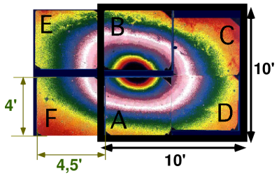
Figure 4: Approximate position of fields A to F with respect to M31.

It turned out that it was impossible to monitor all the fields in both colours each night. We decided to put a priority on the first four fields, with an emphasis on red exposures. Blue images, which require longer exposure times, were less regularly taken. Fields E and F were poorly sampled. We had altogether 76 nights of good weather over the two periods of observation. The number of images taken in each field during the whole survey is summarised in Table 1.

Table 1: Number of pictures taken for each field in both colours, over the two periods of observation.

Field	A	B	C	D	E	F	Z
Red	76	66	60	56	40	32	83
Blue	32	31	24	19	10	8	32

3.3 Pre-processing

Raw data were processed at Pic du Midi during the observation sessions using MIDAS. Mean bias images have been constructed for each night, from a median combination of typically 10 frames, and show a good stability. Mean flat-fields have been made for each run and they correct most of the differences between runs. We come back on this point later.

4 Data reduction

Because observing conditions are never the same for two successive exposures, three corrections have to be applied to the images before pixel light curves can be extracted:

1. A pixel light curve makes sense only if a definite pixel always covers the same part of the sky on all successive pictures to a very high degree of precision (within $0.1\arcsec$). This is never the case for raw data to such an accuracy, and we correct for that by software. We call the corresponding correction geometric alignment.

2. Atmospheric conditions are never the same. In particular, the absorption of light and the sky background change significantly from one exposure to the other (in particular with the moon). The corresponding correction is called photometric alignment.

3. Seeing changes from night to night and this must also be corrected for. However, when dealing with large enough super-pixels far from bright stars it can be neglected in a first step.

Reference image

To apply geometric and photometric alignment, one must choose a reference image. We have chosen images taken on October 26 1994, because observing conditions were good and all fields A to F were available in both colours.

4.1 Star detection and seeing

Figure 5: The seeing for the 1994 and 1995 runs.

To find out a maximum of stellar objects on our pictures, we used an adapted version of the program PEIDA, developed by one of us within the EROS collaboration (Ansari [1994]), which is optimised to process quickly a large number of images. The main changes we had to implement concern the small number of resolved stars (around 50 per field) and the strong gradient of the background, which compelled us to rethink the star detection.

This treatment left us with 56 stellar objects on the reference image of the A field. Each object plus its background was then fitted by a two-dimensional Gaussian PSF plus a plane ($9$ parameters altogether). In this way we get the value of the full width at half maximum (FWHM) for each object.

The next step was to distinguish the “real” stars from other types of objects such as globular clusters, which would artificially increase the average seeing of the picture. We did so using the following discriminating method: if on most pictures the FWHM of an object was significantly above the average, it was removed from the average estimate, and the process was iterated. After this treatment, we ended with a total of 32 “real” stars in each of our pictures of the A field.

This procedure allowed us to discard a few bad images, where the $\chi^{2}$ of the PSF fit was poor for most of the 32 stars. We were left with 64 exposures of good quality for the A field, for which the average seeing for the 1994 runs was $1.5\pm 0.4\,\arcsec$, and $1.6\pm 0.4\,\arcsec$ for the 1995 runs. Fig. 5 shows the evolution with time of the seeing in 1994 and 95, and the distribution of the seeing for both years combined.

Seeing is highly variable and this is a major problem. As mentioned earlier, we cope with these seeing variations by working with super-pixels $2.1\arcsec$ wide obtained by replacing each elementary pixel by the square of $7\times 7$ elementary pixel centered on it. Far from bright stars, this is sufficient for seeings smaller than $1.8\arcsec$, even if we expect to do better in the future.

4.2 Geometric alignment

Figure 6: Dispersion of the difference of star positions between two images after geometric alignment

Geometric alignment involves a two steps procedure:

1. On the reference and the current images, one detects as many bright stars as possible, one identifies them on the two frames, and one computes the general linear transformation in two dimensions, sometimes called the “Turner tranformation”, that corrects for any translation, rotation and scale change between the current and the reference images.

2. The Turner transformation of the current image to the reference image is implemented by linear interpolation. In general, this can become very complicated as each pixel is not only translated but also scaled and rotated. However, rotations and scale transformations are very small and, although they are important for the position of the transformed pixel, the changes they induce on the pixel orientation, size and shape may be neglected.

This geometric alignment is quite successful as can be seen in Fig. 6. The dispersion of the differences in star positions on two images, after alignment, is of the order of 0.3 pixel, that is $0.1\arcsec$. However this dispersion is dominated by the uncertainty on the determination of the position of each star, therefore the precision of the geometric alignment is better than $0.1\arcsec$

a

b

Figure 7: The matching of pixel histograms before (a) and after (b) photometric alignment

4.3 Photometric alignment

In general, photometric alignment is performed assuming that all differences in instrumental absorption between runs have been removed by the correction for flat fields. In this case one may assume the existence of a linear relation (supposing identical seeing) between the intensity in corresponding pixels of the current and reference images:

$$F^{\mathrm{reference\ image}}_{\mathrm{pixel}}=a\,F^{\mathrm{current\ image}}_{\mathrm{pixel}}+b\ .$$ (20)

Here $a$ is the ratio of absorptions (due to variations of the atmospheric transmission and/or airmass effects) and $b$ the difference of sky backgrounds (due to moon phases, and/or variations of the atmospheric diffusion) between the reference and the current image.

The usual way to evaluate $a$ is to compare the total intensities of corresponding stars on the two pictures. However, we cannot get in this way a precision better than a few percent on the factor $a$, because the photometry can be done only on about 50 stars and is difficult on each star, because they are faint and the background is very steep. For this reason, we devised an original global statistical approach to tackle the problem, global in the sense that we take into account all pixels, and not only a few resolved stars. The two methods give equivalent results, but the statistical approach allows to push the precision to about 0.5%.

Statistical approach

Assuming relation (20), the variance $\sigma^{2}$ and the mean value $<\!\mathrm{image}\!>$ of the histograms of pixel intensities on the two images are related by:

$$\sigma^{2}_{\mathrm{reference\ image}} = a^{2}\,\sigma^{2}_{\mathrm{current\ image}}$$ (21-a)

$$b = <\mathrm{reference}>-\,a<\mathrm{current}>.$$ (21-b)

Relations (21-a,21-b) are valid only when the main cause of variance is the gradient of the surface brightness of M 31. The photon noise and fluctuations due to seeing variations can in principle invalidate equation (21-a). However, in our case, the luminosity gradient of the bulge of M 31 largely supersedes all other causes of variations. The efficiency of this procedure is illustrated in Fig. 7: pixel histograms, for four pictures, that look very different before treatment coincide down to small structures after photometric alignment, using only the two parameters $a$ and $b$.

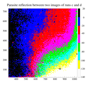
Figure 8: The residual gradient between runs c and d

4.4 Filtering out of large spatial scale variations

Reflected light

After photometric alignment, there remains a slight gradient in the difference between two images of different runs. This is particularly obvious between runs c and d, when we had to take ISARD down and tune its mirrors. This resulted in a substantial gain of luminosity but introduced a significant gradient between images of runs c and d (Fig. 8).

We think that this residual gradient is due to reflected light for the following reasons. i) It is not cured by the usual debiassing and flat-fielding procedures. ii) Its shape depends on the field but seems constant for each field in a given run. iii) Its intensity seems proportional to the overall luminous intensity.

Median background image

To cope with the problem, we construct for each frame a background image where the stars are removed using a median filter. We take a $41\times 41$ window for the median filter, that is with a surface much larger than that of the largest seeing disk, therefore all stars but the very brightest completely disappear. We then subtract from each frame its background image and add that of the reference frame.

High spatial passband filter

This procedure filters out variations of low spatial frequencies: it insures that, relative to the reference image, all variations on scales larger than 40 pixels are very strongly suppressed whereas variations on scales smaller than 20 pixels are fully preserved. The only remaining differences between images come either from short scale fluctuations (seeing variations around stars and around surface brightness fluctuations, or photon noise) or from varying stellar objects.

Residual gradient and the alignment coefficient $a$

Because of this residual gradient, the sky backgrounds of two images do not stricly satisfy Eq. (20). This introduces a systematic error on $a$ when comparing different runs. This error, however, remains smaller than the error arising from matching resolved stars. As all images have been brought to have the same median background, the error on $a$ only affects the difference of the super-pixel intensity with this background and not the total super-pixel intensity. In other word, the systematic uncertainty on $a$ does not alter our ability to detect variations, but it limits our precision on the time evolution of a variation, once detected.

The pixel stability in time achieved after the processing presented above is described in section 5

4.5 Absolute photometric calibration

Absolute photometric calibration is, strictly speaking, not necessary for microlensing searches which rely solely on the detection of relative luminosity variations in time. Nonetheless, to study the nature of the variable objects we detect, it is necessary to know their absolute magnitude.

We took images of the Palomar-Green PG1657+078 calibration field from Green et al. (1986) on 28 July 1995 (calibration day). To determine the flux of reference stars reported in Landolt ([1992]) UBVRI photoelectric observations, we used the same procedure as for the study of seeing (see section 4.1) except that the fit with a gaussian plus a plane is used only to determine the plane that fits the background, the flux of the star is then obtained by subtracting the estimated background to the observed total flux under the star. The photometry obtained in this way turns out to be much more stable among different images. The colour equations for the Johnson R and B magnitudes, denoted $m_{R}$ and $m_{B}$, are:

$$\begin{array}[]{cll}m_{R}&=&\alpha+r+\beta(b-r)\\ m_{B}-m_{R}&=&\gamma+\delta(b-r),\end{array}$$ (22)

where $r$ and $b$ are the instrumental magnitudes with the Gunn r and Johnson B filters:
$r\mbox{ or }b=-2.5\log F_{\mathrm{star}}^{\mathrm{red\ or\ blue}}$.
We find, using a $\chi^{2}$ minimisation:

$$\begin{array}[]{llllll}\alpha&=&21.29\pm 0.02,&\beta&=&0.05\pm 0.02\\ \gamma&=&0.23\pm 0.03,&\delta&=&0.89\pm 0.03.\end{array}$$ (23)

We then have to transform our results for $\alpha$ to the reference day where atmospheric absorption was different. The final value is:

$$\alpha=20.50\pm 0.05$$ (24)

and the other coefficients are not affected.

5 Light curves

The pixel method relies on the inspection of pixel light curves.

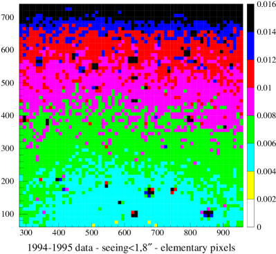
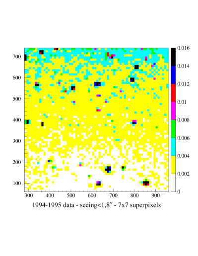
Figure 9: Maps of the relative fluctuation on field A for $(0.3\arcsec)^{2}$ elementary pixels (upper map), and $(2.1\arcsec)^{2}$ super-pixels (lower map).

Light curves are graphs of the variation of pixel intensities. Elementary pixels are small ($0.3\arcsec$), which is very useful to get a good geometric alignment. However, elementary pixels undergo strong fluctuations due to seeing variations that hamper detection of truly variable stellar objects. For this reason we replace each pixel by a super-pixel, as explained in section 2. A convenient size for the super-pixel, in vue of the average seeing of $1.5\arcsec$, turns out to be $2.1\arcsec$, wich corresponds to super-pixels built with $7\times 7$ elementary pixels.

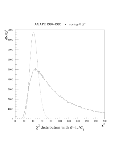
Figure 10: The distribution of $\chi^{2}$ along light curves of field A

Using super-pixels provides a substantial gain in stability. Figure 9 shows maps of the relative fluctuation along the light curve of elementary $0.3\arcsec$ wide pixels, and of $2.1\arcsec$ wide $7\times 7$ super-pixels of field A (Notice that there are as many super-pixels as elementary pixels). On elementary pixels, the dispersion is below 1% on most of the field. For super-pixels, the dispersion drops down to 0.3% in average and even reaches a level below 0.1% in the most stable regions, as announced earlier. It remains everywhere around twice the photon noise.

To compare in more detail the super-pixel fluctuation to the photon noise, we have computed along the light curve of each super-pixel the $\chi^{2}$ of the difference between the intensity on the current image and its average in time. In Fig. 10, we display the distribution of this $\chi^{2}$ for the super-pixels of field A, using two different seeing selections. The error $\sigma$ entering the $\chi^{2}$ is chosen in such a way that the maximum of the distribution of the $\chi^{2}$ coincides with that of the ideal Poisson law. This is achieved for $\sigma\simeq 1.7\sigma_{\gamma}$ where $\sigma_{\gamma}$ is the statistical photon noise. The true distribution shows non-poissonian tails. Clearly there are non-statistical contributions to the fluctuations and a comparison between Fig. 10a and Fig. 10b shows that they are largely due to seeing variations. Further work is in progress to cope with the latter. This non poissonian behaviour is also responsible for the fact that, in going from pixels to super-pixels, one gains less than the factor 7 expected if fluctuations were of pure statistical origine.

We have made the same study replacing super-pixels by a PSF weighted average. The fluctuation is twice larger than with super-pixels, and the tails due to seeing variations in the $\chi^{2}$ distribution are much larger.

Figure 11 illustrates the considerations above with the light curve of a stable super-pixel, keeping only the frames with seeing between $1.1\arcsec$ and $1.8\arcsec$. Super-pixel intensities are in ADU/s (1 ADU/s on a 2.1$\arcsec$ super-pixel corresponds to a surface magnitude $\mu_{R}=22.1$). The R.M.S fluctuation along

Figure 11: The light curve of a stable $2.1\arcsec$ super-pixel. The intensity per super-pixel is in ADU/s ($1.1<\mathrm{seeing}<1.8$).

Figure 12: An example of a variable object.

the light curve is 0.045 ADU/s, to be compared with the average photon noise which is around 0.04 ADU/s. If one keeps all points, irrespective of the seeing, the RMS fluctuation becomes 0.065 ADU/s. The error bars correspond to 1.7 $\sigma_{\gamma}$, that is around 0.07 ADU/s in average.

With this level of stability, we are able to clearly see variations at the level of a few percent as is apparent from Fig. 12. Let us stress the following features of this figure.

1. This light curve shows two clear variations, it is a variable star, not a microlensing.

2. On graph (b), only points corresponding to a seeing between $1.1\arcsec$ and $1.8\arcsec$ have been retained and the light curve appears much smoother than on graph (a).

3. After seeing selection (graph (b)), the first variation can clearly be seen, because of its coherence in time, although it is only about 0.5 ADU/s, that is about 5 times the average error bar in this period.

We see that the the selection criteria we have introduced in our Monte-Carlo simulation in section 2.2 (3 points above $3\sigma$ and one of them above $5\sigma$ ) are indeed realistic. However our present thresholds are much higher, because these criteria would be sufficient if microlensing were the only possible source of variations. This is of course not the case and variable stars are far more numerous. If we used only the criteria of our simulation, we would be swamped by variable objects. Therefore, to isolate microlensing events we have to build filters which reject most of the variable objects but not the microlensing events satisfying our criteria. There are many conditions that can be added, such as:

• the usual conditions of unicity, symmetry and achromaticity

• the quality of fits by a Paczyński curve

• limits on the duration of events expected from MACHO’s with reasonable masses compared with what is expected from simulations (see figure 1).

We are working on that. We will be in a better position after the 30 observation nights we shall have in autumn 1996. Although these nights will be too few and too scattered to allow detection of new events, they will allow to constrain efficiently fits of events that occured in 1994 and 1995

Even events that overshoot by far our criteria would have been extremely difficult to detect by monitoring resolved stars.

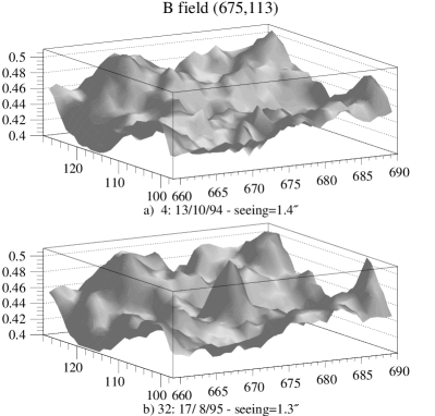
Figure 13: Appearance of a star. The vertical scale is the intensity per elementary pixel, in ADU/s

This is illustrated in Fig. 13. The two dimensional surface plots (a) and (b) map the intensities of elementary pixels around the centre of a detected variation. Plot (a) corresponds to the minimum of the light curve and plot (b) to the maximum. Most structures appear similar on the two plots, which means that they correspond to real structures of M 31. They are the surface brightness fluctuations of Tonry & Schneider ([1988]). At the centre however, a tiny bump, barely visible on graph (a), has grown into a clear PSF-shaped peak on (b). This tells us that we are really looking at a varying stellar object, barely detectable as a resolved star.

Variable stars are interesting in their own right. Numerous variable objects such as the preceding ones have been detected, but we are only beginning to analyse their nature.

Figure 14: Likely cepheid and nova.

Figure 14 shows the light curves of two objects, one of which is probably a cepheid, and the other a nova. We have a host of other cepheid candidates and five novae with peak magnitude and rate of decrease similar to the one shown on Fig. 14, and very similar to the M 31 novae quoted in Hodge [1992].

We also see variations compatible with microlensing (about 20). However at this stage, we are not in a position to claim that we have seen microlensing events for several reasons. First, our lever arm in time is not sufficient to be sure that the variations do not repeat, and even in some cases, to be sure that events are really symetric. The situation will improve with the 30 nights we expect in autumn 1996. Second, we have not yet analyzed the blue light curves, therefore we cannot yet test achromaticity. Figure 15 shows one of these light curves.

Figure 15: A possible microlensing event. The solid horizontal line is the basis level of the super-pixel intensity (in ADU/s), the dashed line lies $3\sigma$ above and the dotted line $5\sigma$ above.

The Paczińsky curve on Fig. 15 corresponds to a star of absolute magnitude M=-2 amplified by a factor 6 at maximum and with an Einstein time scale $t_{E}=65$ days. These number are not well determined because of a parameter degeneracy for high amplification events (see for instance Gould [1995]), which is the case of most events we can detect. A time scale and a maximum amplification twice as large associated with a star twice fainter would fit just as well. However the time scale cannot be much shorter, because the star should be brighter and would be seen more clearly before the lensing begins. The effective time $t_{\mathrm{eff}}$ is 19 days if one measures it between real points of observation where the signal to noise ratio is higher than 3, and 40 days if one refers to the time during which the Paczińsky curve remains at 3 $\sigma$ above the background. This effective time is a powerful mean to eliminate fake microlensing events: our simulation tells us that $t_{\mathrm{eff}}$ should be smaller than 60 days for lenses with masses around 0.08 $M_{\odot}$. The numerous time gaps we have in the observations make it difficult to find short events, and it is important to our approach to have as few gaps as possible in the time sampling.

6 Conclusion

On the basis of data taken during two autums at the 2 metre telescope Bernard Lyot at Pic du Midi, AGAPE has proven that the pixel method works. Super-pixels, taken $2.1\arcsec\times 2.1\arcsec$ large to minimise the effect of seeing variations, have a level of fluctuation not larger than 1.7 times the photon noise. On the brightest super-pixels this fluctuation is not more than 0.1% of the photon background. With such a stability, our simulations predict that we should see around 10 events in the direction of M 31 for lenses with $0.08M_{\odot}$ masses, an event beeing called detectable if its light curve remains 3 $\sigma$ above the background for at least 3 consecutive points and reaches 5 $\sigma$ at one of them. Such variations are clearly detectable from their time coherence, even if more work is needed to separate microlensing events from other kind of variations. We are already detecting hundreds of variable stellar object in M 31, in particular cepheids and novae. They are currently beeing analysed.

To exploit the full power of our method, we are exploring the possibilities of launching an observation with a wide field camera on an instrument were we could get a very regular and short time sampling, and a lever arm of several years. We would then be able to make a map of the halo of M 31, which would be of considerable interest for halo model builders.