A new family of non–linear filters for background subtraction of wide–field surveys

Abstract

In this paper the definitions and the properties of a newle dedicated set of high-frequency filters based on smoothing-and-clipping are briefly described. New applications for reduction of wide–field 2048$\times$2048 CCD spectral and direct images of a new deep survey KISS are also presented.

1 Introduction

The reduction of 2D astronomical images requires a proper subtraction of the night sky. Even a perfect flat-field may correct only chip inhomogeneities or optical vignetting on the CCD frames but there are many other sources of additive noise that can not be removed with flat-fielding; thus, there is a general problem of building a correct background which includes such additive noise. Sometimes it is possible to use a 2D polynomial approximation or other fittings to take into account a small gradient across the field, but, in general, such methods do not help much, and this task can not be solved by the usual methods incorpoprated within standard reduction systems such as IRAF or MIDAS.

The possible sources of the additive noise include a gradient throughout a large field ($\geq 1^{\circ}$) due to vicinity of the Moon, traces of light clouds when the weather is not perfect, faults of the electronics, optical ghosts inside telescope optics, etc. All these effects create large-scale features up to the size of whole frame. Some known extra problems rise when a Schmidt telescope and an objective prism are used; one can see many reflections from bright stars out of a studied field, scattered and reflected by many optical surfaces light. Of course, they can not be removed with flat-fielding because of their additive nature. On the other hand, an application of an adaptive filter requires good flat frames without any gradients (Lorenz et al. 1993). Usually a threshold is applied in order to create a correct mask for a reasonable estimate of the noise.

In 1994, two of the authors (A.K. and V.L.) ran into these severe problems processing data from a new survey KISS (KPNO International Spectral Survey (Salzer et al 1994). KISS is a newly dedicated spectral survey. It utilizes the Burrel Schmidt telescope with a 2^∘ objective prism, 2048$\times$2048 CCD, and a special 4800$\div$5500 Å filter blocking strongest lines of the night sky. KISS aims to search for emission-line galaxies in the region of the Century Survey in a 1^∘ slice going through the Northern Galactic Pole.

There are several known ways how to build a background or to avoid it during processing. They may use wavelet transformation, adaptive filtering, median filtering, etc. (cf. Bijaoui, 1980; Slezak et al., 1990; Coupinot et al., 1992; Lorenz et al., 1993). Good results for removing some large-scale features had been achieved with fast 2D median filter (and filters based on any other order statistics) (Pasian, 1991). Nevertheless, these algorithms are very time consuming due to 2D nature when large features should be removed. We consider the problem of background fitting as a problem of robust estimation of an average value in the window where objects of interest are mixed up with all other sources from the background noise.

The authors use another approach called the smoothing-and-clipping algorithm (SAC), considering any image as a set of independent rows or columns, filtering them as 1D structures, and combining them after the filtering. Initially this algorithm had been used for reduction of 1D radio data for the detection of weak sources during the deep survey conducted with the RATAN–600 radiotelescope (Erukhimov, Vitkovsky and Shergin, 1990; Verkhodanov et al. 1992, 1993) in the Special Astrophysical Observatory. The algorithm has been modified by the authors for the application to 2D optical images and 1D optical spectra.

For radio data a signal consists of the positive sources detected above a certain background level plus noise. Data processing is then a removal of such a background and the robust estimation of the remaining sources. There is a certain similarity between a single row (column) of CCD (with superimposed stars and galaxies) and a radio record. The reflections of a bright star inside the telescope optics form a background, which is an additive signal, that should be removed when processed. There are some differences between optical and radio data. The latter are always supposed to have a constant noise level. CCD data, on the other hand, may have a variable noise. For example, observations with noticeable vignetting after flat-fielding have a quite different noise over the field, and this fact has to be taken into account to get the correct S/N value.

This approach might be applied to optical spectra to fit the optical continuum as some sort of background. But such spectra are more complicated due to possible emission and/or absorption lines and to the more sophisticated shape of the real spectral continuum. So, for optical range there is always a variable noise along the spectrum because of variable spectral sensitivity and may be also be other effects. They required us to modify our algorithms to include a variable noise, their description will be publushed elsewhere, this paper deals with the processing of 2D images.

2 Description of the algorithm

In general we mean not single but a family of such SAC algorithms and all of them specified by two main steps: smoothing and clipping, repeated iteratively.

Consider some definitions before the algorithm description:

• Array S(x) is an inputed 1D spectrum or initial data (row or column); define it as $\overline{S}$.

• Let there be $\lambda$ a window width of the smoothing algorithm. We suppose $\lambda$ is larger than any source width (emission or absorption line width for a spectrum).

• Clipping procedure of the algorithm deals with the noise level $\sigma(x)$. In the general case it changes from point to point for input data and we define it as a vector $\overline{\sigma}$.

• $\overline{W}_{n}$ is a vector of weights for the n-th iteration smoothing. The initial value $\overline{W}_{0}=1$, and $\overline{W}_{0}$ runs in the range from 1 to 0. The weight vector shows a relative contribution of each point during smoothing.

Then SAC algorithm performs following steps for every iteration:

1. Calculates an input vector $\overline{C}_{i}$ for the $\bf i-th$ iteration of smoothing as:

   $$\overline{C}_{i}={\cal F}(\overline{S},\overline{W}_{i-1})$$ (1)

   The index $\bf i$ is the number of the iteration. $\overline{W}_{i-1}$ is a vector of weights calculated in the previous iteration. In the simplest case the function $\cal F$ is calculated as a product of each vector component – ${\cal F}_{k}=S_{k}*W_{k}$, where $k$ is the $k$-component.

2. Smoothes $\overline{C}_{i}$. Define $\Lambda_{i}(\lambda)$ as the smoothing operator. Index $\bf i$ shows that generally $\Lambda_{i}(\lambda)$ may depend on iteration number. Obviously the operator $\Lambda_{i}(\lambda)$ depends on the input parameter $\lambda$. The result of such an operation upon input vector $\overline{C}_{i}$ is:

   $$\overline{B}_{i}=\Lambda_{i}(\lambda)\>\overline{C}_{i}$$ (2)

   For the first iteration, $\overline{C}_{1}=\overline{S}$, according to definition.

3. Subtracts $\overline{B}_{i}$ from the input data vector $\overline{S}$:

   $$\overline{D}_{i}=\overline{S}-\overline{B}_{i}$$ (3)

4. Calculates a new function of weights as a non-linear transformation $\Phi_{i}(\overline{\sigma})$, which is a function of input noise $\overline{\sigma}$ and the number of the iteration in a general case:

   $$\overline{W}_{i}=\Phi_{i}(\overline{\sigma})\>\overline{D}_{i}$$ (4)

5. Goes to the next iteration. SAC algorithm does not converge as a rule; thus, one should choose when to stop the procedure.

As was aforementioned, SAC presents a family of filters. There are several possible smoothing and weighting methods. In practice we explored the following methods for smoothing:

• simple boxcar average;

• median average (Erukhimov, Vitkovski and Shergin 1990);

• convolution with Gaussian–like expanding profile;

• weighted least squares polynomial approximation of 1$\div$15 degrees.

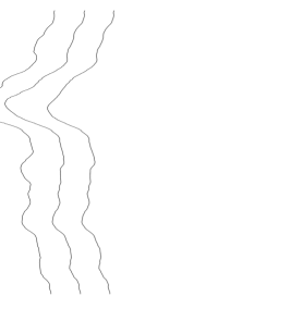
To calculate the weights some empirical transformations are used. They may be specialized to cut emission, absorption or both. The authors employ their own empiric function plotted in Figure 1 for all smoothing methods. We should make two notes: a) there is a known problem of smoothing on edges; this problem should be solved in any particular case, b) for optical data the noise may be variable throughout the image (spectrum); thus, our program has been modified for such a case.

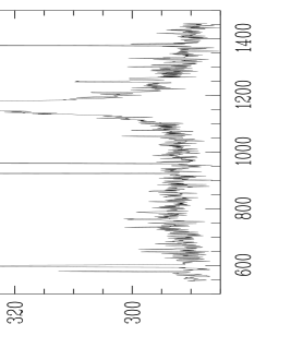
Figure 2 illustrates some iterations for 1D data (a single row from KISS CCD data). It is clear that the result the after 5-th iteration is quite satisfied.

Figure 1: Empirical transformation (weighting) used by authors. Abscissa value is a difference between initial data and background estimation for the i-th iteration in terms of input noise for the k-th element of the vector.

Figure 2: An example of SAC filter with a Gaussian smoothing window, $\lambda=60$ pixels (the bar in the up–left corner shows the smoothing window size). The upper figure is a portion of an extracted CCD row in pixels, the bottom figure shows the 1-st (simple convolution of the data with Gaussian profile), 2-nd, 5-th and 10-th iterations, all plots shifted arbitruary along the ordinate axis. It is evident that after the 5-th iteration the results practically do not change. All features smaller than a window size are smoothed very quickly. The bright saturated star, chosen on the upper right part of Figure 3, has a profile width somewhat larger than $\lambda$ and te algorithm clips only the narrow part of this profile

3 Application and tricks

The developed software is available both as a C subroutine and as an installed MIDAS environment command (see Appendix).

This software is used to process KISS CCD direct images and taken with an objective prism. Figure 3 presents a quite successful result of SAC cleaning for a direct image. It is evident that all imperfections — such as noticeable jump of the background due electronic ”gliters” during CCD read-out, the halos of bright stars and a gradient in the low left corner pof the frame were corrected to an accuracy better of greater than 0.1%.

The authors tested the program with different platforms. Their experience showed that, thanks to the 1D approach, SAC may be used even with small PC computers installed with MIDAS. The total time does not depend on the window size for simple boxcar average, and the typical time is only about a few minutes for a 2K$\times$2K frame. For Gaussian smoothing, the time depends strongly on window size $\lambda$. Table 1 sums up typical times for two sizes, 2K$\times$2K images, and 3 different computers. For polynomial smoothing, the procedure time is about 4 times quicker than for Gaussian.

Table 1: Typical time of SAC performance on different platforms

Platform	RAM	Time for	Time for
	size	$\lambda=60$ pixels	$\lambda=90$ pixels
(1)	(2)	(3)	(4)
SUN–server NOAO	128 Mb	55 min	2.5 hours
Sparc–20	64 Mb	45 min	2 hours
Convex	900 Mb	2 hours	5 hours

Some tricks of SAC perfomance include:

1. The fastest algorithm is boxcar averaging but this method is the roughest. The compromise may be reached using boxcar averaging as a start and Gaussian smoothing in the end. The polinomial smoothing has a intermediate quality comparing with the others.

2. For a 2D frame there are two sizes for a source; thus, one may chose the direction, X or Y, to smooth the image. For instance, objective prism spectral images of stellar objects with have typical sizes 5x45 pixels; thus, it may be recommended to smooth across the dispersion.

3. When there are some artifacts like spikes of bright stars, it is better to select the dominant direction to remove them. In a unique case, such as tracks of a satellite or a plane, we recommend to rotate a frame along such tracks and then apply SAC.

4. The program needs only an innitial estimate of the noise, not a precise value. The usefull of this feature was shown in Figure 3 where different image parts has different amount of noise (difference was about 20%).

The authors (A.K. and V.L.) are grateful to the staff of the Astrophysical Institute Potsdam for their hospitality and the possibility to use their Convex computer to process KISS data.

Figure 3: KISS direct image for field $\alpha=14^{h}45^{m}$ before (upper) and after (lower) SAC cleaning. The small jump on the upper image of about 1.3% was caused by an elecronics failure during read–out. The noise value is a little different for two parts of initial image ($\sigma_{up}$=6.49, $\sigma_{down}$=7.78), but the SAC does not need it to be precise. For an initial value $\sigma_{aver}$ was taken for the SAC program.

Appendix A MIDAS procedure of SAC

The command works both for versions 2D image and for real 1D spectra. For 2D images the parameter for spectrum type should be ”both”. The working version of this command had been installed in SAO on PC computers and Sparc 20 and in AIP on the Convex machine.

@s contin  inp_image  out_image  smooth_wnd  noise_level
Ψ   iter_numb  bgd_and_out_type  smooth_mode  smooth_step

where:     inp_image   - input frame
Ψ   out_image   - output frame
Ψ   smooth_wnd  - width of smoothing window
Ψ   noise_level - noise estimation
Ψ   iter_numb   - number of iterations
Ψ   bgd_and_out_type - two characters (default - "bb") :
Ψ      bgd_type   -   a/e/b (for "absorbtion" or "emission" or "both")
Ψ      out_type   -   r - residuals    b - background itself
Ψ   smooth_mode   -  <0 - quick-rough mode, boxcar averaging
ΨΨΨ    =0 - slow mode, convolution with Gaussian window
ΨΨΨ    >0 - fitting polynom power (< 15)
Ψ   fitting_step-  step of fitting polynom locations (< smooth_wnd/2)

Ψ   Type "help" as the first parameter to get short help

References

- [1] Bijaoui A., 1980, Astron.Astrophys., 84, 81
- [2] Coupinot A., Hecquet J., Auriere M., Futaully R., 1992, Astron.Astrophys., 259, 701
- [3] B.L.Erukhimov, V.V.Vitkovskij, V.S.Shergin, 1990, Preprint SAO RAS, 50
- [4] Lorenz H., Richter G.M., Cappaciolli M., Longo G., 1993, Astron.Astrophys., 277, 321
- [5] Fabio Pasian, 1991, 3-rd ESO/ST-ECF Data Analysis Workshop, p.57
- [6] Verkhodanov O.V., Erukhimov B.L., Monosov M.L., Chernenkov V.N., Shergin V.S., 1993, Izvestiya SAO, Astrofiz. Issl, (Bulletin of SAO, Russia), 36, 132
- [7] Verkhodanov O.V., Erukhimov B.L., Monosov M.L., Chernenkov V.N., Shergin V.S., 1992, Preprint SAO RAS, 87
- [8] Salzer J., Lipovetsky V.A., Boroson T., Kniazev A.Yu., Thuan T.X., Izotov Yu.I., Moody J., 1994, BAAS, 26, 916
- [9] Slezak E., Bijaoui A., Mars G., 1980, Astron.Astrophys., 227, 301