Sub-degree Scale Microwave Anisotropies from Cosmic Defects

Abstract

If current ideas about unified field theories are correct, macroscopic cosmic defects may well exist. The observation of such an entity would have enormous significance for our understanding of fundamental physics. This paper points out a novel observable signature of cosmic texture and global monopoles, namely strong hot spots in the cosmic microwave anisotropy pattern on subdegree scales. This signal should be readily detectable by the next generation of anisotropy mapping experiments. The signature arises from overdensities in the photon-baryon fluid generated by the gravitational attraction of the defects. The angular power spectrum of the anisotropy fluctuations on subdegree scales is also calculated, for cosmic string, global monopoles, and texture.

The prospect of accurate maps of the temperature fluctuations on the cosmic microwave sky gives us hope of resolving one of nature’s most profound questions, the origin of large scale structure in the universe. The recently approved COBRAS-SAMBA and MAP satellites, the Very Small Array interferometer, and other experiments, promise to provide cosmological data of unparallelled quality and quantity.

Cosmic defects have been of fascination to theorists ever since it was realised that their presence was generic in unified field theories of high energy physics [1]. Indeed, if current ideas about the unification of forces are correct, cosmic defects in one form or another are almost unavoidable. Two such defects occur in standard model physics - namely electroweak textures and skyrmions, formed as a result of the breakdown of the electroweak and strong chiral symmetries respectively. Neither of these is relevant to the problem of structure formation, but analogous defects formed through the breakdown of symmetries at much higher, grand unification energy scales, do give rise to interesting theories of structure formation in the universe [2]. Cosmic strings are the best known of these, but global monopoles and textures are also promising candidates [3]. A period of inflation can, but does not necessarily, dilute the defects to unobservably low densities. For example, recent work has has shown that they may be efficiently produced during the reheating process following inflation [4]. The imminent maps of the microwave anisotropy offer a unique observational window on cosmic defects, and the possibility of discovering whether any of these relics of unification have survived within our observable universe.

As mentioned, macroscopic cosmic defects provide a possible mechanism for structure formation which is a valuable alternative to the more popular scheme based on inflation. The two theories could hardly be more different - where the inflationary scheme is inherently quantum mechanical, the cosmic defect mechanism is purely classical. The formation of fluctuations during inflation involves linear physics, whereas the defect theories are highly nonlinear. Related to this, the inflationary fluctuations take the form of Gaussian random noise, whereas the defect induced fluctuations are highly non-Gaussian.

Recent work has emphasised further fundamental differences. First, the defect theories are highly constrained by causality, so that the fluctuations are completely uncorrelated beyond the horizon scale at all times [5], [7], [8], [9]. And second, the nonlinearity of the theories means that the evolution of each Fourier mode $\vec{k}$ in the perturbations is different, and cannot be predicted on the basis of the initial conditions of that mode alone, because all the modes are coupled. This property is referred to as ‘incoherence’ - modes of the same wavenumber $k$ do not follow identical time evolution [7]. This has the effect of smearing the ‘Doppler’ peaks in the angular power spectrum of the anisotropies, caused acoustic oscillations in the photon-baryon fluid just prior to recombination.

Advances in computer power have recently made possible realistic calculations of microwave anisotropy maps in the defect theories. Following the COBE satellite results, several groups have reported calculations for the large angle cosmic microwave anisotropy patterns [10], [11], [12], [13]. Unfortunately, the information available in a map with 7 degree resolution, such as the COBE 4 year maps, appears too limited to meaningfully discriminate between the inflationary and defect theories - all these theories are compatible with the COBE measurements.

The first realistic computations of degree-scale CMB anisotropy from cosmic defects were reported some time ago [14]. These were performed assuming a fully ionised universe, mainly for technical simplicity. The present paper shall consider instead the case of standard recombination, in which much more small scale structure is visible, on scales down to 10 arc minutes. Below this scale, even with standard recombination, photon diffusion on the last scattering surface begins to blur the anisotropy pattern.

At early times, redshifts $Z>>1100$, photons are tightly coupled to ionised matter, forming the photon-baryon-electron fluid. As the universe cools, the electrons and baryons undergo ‘recombination’ forming neutral atoms, and the plasma quickly becomes transparent. In the approximation that recombination happens instantaneously, the microwave anisotropy seen in a direction ${\bf n}$ on the sky is given by

$$\frac{\delta T}{T}({\bf{n}})=\frac{1}{4}\delta_{\gamma}(i)-{\bf{n\cdot v_{\gamma}}}(i)-\frac{1}{2}\int_{i}^{f}d\tau\dot{h}_{ij}{\bf n}^{i}{\bf n}^{j}$$ (1)

where $\tau$ is conformal time, $\delta_{\gamma}$ is the photon fluid density contrast, and ${\bf v}_{\gamma}$ the velocity of the photon-baryon fluid on the spherical shell representing the ‘surface of last scattering’. The term ${1\over 4}\delta_{\gamma}$ is the intrinsic temperature contrast, and the second term is the Doppler effect. The last term involves the time derivative of the metric perturbation $h_{ij}$, and represents the change in the proper path length due to a time-dependent gravitational field along the line of sight. This is the Sachs-Wolfe effect[15].

Equation (1) is written in the synchronous gauge, sometimes criticised in the literature because it possesses residual gauge freedom. However, this gauge is well suited to the cosmic defect theories discussed here. In these theories, the universe is assumed to be perfectly smooth before the symmetry breaking phase transition which produced the defects. The perturbation variables can therefore all be set to zero. This choice, called initially unperturbed synchronous gauge has no residual gauge freedom. The nice property of this gauge is that the Einstein equations are then completely causal, with the value of all perturbation variables at a given spacetime point being completely determined by initial conditions within the point’s backward light cone. Gauges like the Newtonian gauge suffer from the problem that perturbations due to anisotropic stresses, which are generally present in these theories, propagate acausally [16].

In initially unperturbed synchronous gauge, all the variables in equation (1) have an unambiguous physical meaning. The contrast $\delta_{\gamma}$ in the photon density is that observed by a local freely falling observer (for example a cold dark matter particle). Likewise $\bf{v_{\gamma}}$ is the velocity of the photon-baryon fluid with respect to cold dark matter. There is an additional Doppler term which may be attributed to the peculiar motion of the dark matter, but that arises from an integration by parts of the last term [14].

The split represented in equation (1) is useful in a causal theory, because the first two terms are completely determined by the source for perturbations within the backward sound cone, with comoving radius $\int_{0}^{\tau_{rec}}c_{s}(\tau)d\tau$, with $\tau_{rec}$ the conformal time at recombination and $c_{s}<1/\sqrt{3}$ the speed of sound in the photon-baryon fluid. The last term depends on the perturbation source over a much larger region of spacetime, filling the backward light cone of each point on the photon’s trajectory. Apart from the earliest contributions to the integral, in the vicinity of the last scattering surface, there is little correlation between the first two terms in (1) and the Sachs Wolfe integral. Furthermore, the latter produces an approximately scale invariant angular power spectrum, monotonically falling, and with no ‘Doppler’ peaks (see ref. [14]). It is therefore unlikely to be important in influencing the position of the peaks in the power spectrum produced from the first two terms, and is a subdominant effect in the height of the peaks. I have checked this explicitly in the texture model of reference [5], where the approximation of ignoring the Sachs-Wolfe integral in (1) yields a primary peak in the angular power spectrum higher than the full result, but only by 20 per cent. Note that this approximation is certainly not good for a theory like inflation, where there are large correlations on superhorizon scales.

In this paper I report on calculations of the first two terms alone, which dominate the anisotropy on scales from a degree down to several arc minutes. Including the Sachs-Wolfe integral is certainly a goal for future work, but the memory and CPU requirements would have severely compromised the resolution available. The calculational technique involves an improved nonlinear sigma model code in which local stress energy conservation holds to an accuracy of a few per cent, and is quadratically convergent in the timestep. This is coupled to a three dimensional leapfrog code for the dark matter (taken to be ‘cold’ dark matter), neutrinos (treated as a fluid with viscosity), and the photon-baryon-electron fluid, with a time-varying speed of sound. For strings, the flat spacetime code of ref. [14] is employed, with the modification that an extra fluid (with $c_{s}^{2}=1/3$) is introduced to account for the energy and momentum lost by the strings due to a) the expansion of the universe, and b) the emission of small loops and gravitational waves. This ensures exact local conservation of the source stress energy tensor. Whilst the string network used is reasonably realistic, having for example similar scaling density to that reported in expanding universe codes, the string results have considerably larger systematic uncertainties than those for texture and monopoles.

Simulations were performed for $256^{3}$ boxes, with the horizon at last scattering representing 45 grid spacings. Tests of the source stress energy tensor indicate that the fluctuating part achieves scaling form after as little as 5 grid spacings, which is still significantly before matter-radiation equality. At the instant of recombination, slices across each box were taken at intervals of 32 grid spacings (no correlation was apparent between neighbouring slices), with the Doppler and intrinsic terms stored separately. This produced 8 maps per simulation. The maps are available via ftp from the author.

The four colour Figures show representative maps for strings, global monopoles, textures and standard cold dark matter. The maps are 10^o square, and have been smoothed with a Gaussian of FWHM 12” (5 grid spacings), to simulate the effect of Silk damping. The maps show the temperature contrast $(\delta T/T)$ in units of one standard deviation, arising from the first two terms of equation (1). In each case the cosmological parameters used were $\Omega=1$, $\Omega_{B}=0.05$, $h=0.5$, $\Lambda=0$. As mentioned above, because the Sachs Wolfe integral has been omitted, these maps have slightly less power than they should on scales above one degree or so. But the most striking features in the maps occur on smaller scales, and these should be accurately represented.

There are two ways in which the theories studied are manifestly different. First, the scale of the structure present in the maps increases as one goes from strings to monopoles, textures and standard inflation. This is a reflection of the differences in angular power spectra, and in particular the shift in the primary peak in the power spectrum (Figure 5). Second, the texture and monopole maps show clear ‘hot spots’ in excess of 5 or 6 $\sigma$, which would be highly improbable in a Gaussian theory. The fact that hot spots, and no cold spots are seen, is a simple result of the fact that the defects themselves represent localised concentrations of energy, which attract the photon-baryon fluid, and cause a local rise in the local density and temperature. Localised defects, like unwinding textures or annihilating monopole-antimonopole pairs, do so more effectively than extended objects like strings. After a hot spot is produced, I have established that it is the presence of the somewhat diffused surviving defect stress energy in the region that prevents the photon density from oscillating negative and producing a cold spot.

Let us now discuss quantitative measures of these differences. The first is the angular power spectrum, defined as the ensemble average $C_{l}=<|a_{lm}|^{2}>$, where the temperature on the sky is expanded in spherical harmonics as $(\delta T/T)(\theta,\phi)=\Sigma a_{lm}Y_{lm}(\theta,\phi)$. In Figure 5, the quantity $l(l+1)C_{l}$, constant for a perfectly scale invariant spectrum, is plotted against $l$. Multipole index $l$ is converted into an angular scale by noting that on small scales, the sky is nearly flat, and $l$ is effectively the two dimensional wavenumber. Modes with index $l$ have a wavelength on the sky of $\Delta\theta=(2\pi/l)$. Figure 5 shows the ensemble averaged power spectra for the four theories considered here. Each has been normalised to the COBE 4 year data, using the results of [11] for monopoles and texture, and [14] for strings [18]. The curves show the average of 3,4 and 6 runs (producing 8 maps each) for strings, monopoles and textures respectively. The fractional statistical error in the power at each $l$ is $\pm\sqrt{2/N}$ for $N$ uncorrelated maps - for the available ensembles this works out at approximately 20 per cent for textures, 25 per cent for monopoles, 30 per cent for strings. The dashed line shows the result for the standard inflationary model.

The solid line shows the result for the texture model calculation presented in [5], when it is used to compute the same contributions to the anisotropy studied here. The $C_{l}$’s from the model have been multiplied by a factor 0.6 after COBE normalisation (this correction is consistent with the estimated systematic errors quoted in [5]) - it appears that model overestimates the height of the primary peak by this factor. The position of the primary peak is however in excellent agreement with the predictions of refs. [5], [6]. Note that the approximation employed here of neglecting the Sachs-Wolfe integral significantly underemphasises the second peak (at $l\sim 650$), but not the third, which also appears visible in the full texture simulations.

The higher peaks do appear to be present in texture simulations at the locations expected from the model of [5], but the statistics so far obtained are inadequate to fully resolve them. One should also worry about effects due to the non-scaling initial conditions, and other sources of noise which would tend to smear the peaks. The techniques used here are not ideal for quantitatively determining the extent of the decoherence of the defect-induced perturbations (nor indeed the $C_{l}$’s themselves), for which a Fourier space approach would be preferable. Nevertheless, secondary peaks are apparently visible in the intrinsic temperature term alone (dashed lines). There are also hints of secondary peaks in the cosmic string theory (the spacing between the spikes, $\Delta l\sim 280$ is what one expects for coherent acoustic oscillations - one has $\Delta(c_{s}k\tau_{rec})\sim\pi$, and $\Delta l\sim\Delta(k\tau_{0})\sim 50\Delta(k\tau_{rec})$ ), but the statistics are again insufficient for any firm conclusion. It is notable that the power spectra for individual maps frequently show very clear peaks, with the appropriate spacing $\Delta l\sim 280$, but these are displaced from map to map in such a way that the ensemble average is smoother. This seems to be a clear signal of decoherence [7].

The calculations reported here, as mentioned above, significantly underestimate the total power at lower values of $l$. The scale invariant plateau produced by the Sachs-Wolfe integral is at $l(l+1)C_{l}\sim 7\times 10^{-10}$. For $300<l<2000$ or so for textures and monopoles, and $400<l<2000$ for strings, the $C_{l}$’s shown include the dominant effects, but the Sachs-Wolfe integral may add $\sim 20-40$ per cent to the power. Above $l\sim 2000$, at least in the case of strings, the structure of the defect-induced Sachs-Wolfe signatures produced after last scattering start to contribute, leading to a tail of high $l$ power which is unaffected by Silk damping [19]. It is interesting to compare results with Bouchet et. al. [20], who calculated only the Sache-Wolfe integral for strings, in a Minkowski-space approximation. They concluded that the contribution was roughly scale invariant, and the rms anisotropy from the interval $[Z,2Z]$ was $\sim 6G\mu$, with $G$ Newton’s constant and $\mu$ the string tension. Here I find the rms from the the intrinsic and Doppler terms to be larger, $\sim 13G\mu$. Thus the contributions studied here are likely to mask the linear signatures of the strings, at least on angular scales above 10 arc minutes. These conclusions are consistent with model calculations of the string anisotropy power spectrum [17].

The number of maxima and minima of height $\nu\sigma$, where $\sigma$ is the standard deviation, provides a simple quantitative test of the nonGaussianity of the maps. For a Gaussian theory, the number of peaks and minima per unit area, $dN/d\nu$ is straightforwardly calculable in terms of moments of the power spectrum [21]. In this case the curves for maxima and minima are simply related by the replacement $\nu\rightarrow-\nu$. Figure 6 shows the number of maxima and minima for the theories studied here. While the curves for minima take a form very similar to what one expects for a Gaussian theory, the curves for maxima show a clear excess of high peaks, especially marked in the monopole and texture theories. Note that this skewness was not present in the maps made by Coulson et. al. [14] of the Sachs-Wolfe contribution, it is entirely an effect of the ‘intrinsic temperature’ and ‘Doppler’ terms studied here.

One can read off from Figure 6 how much sky coverage is needed in order to see one of these extreme events. For example, there is approximately one peak in excess of $5\sigma$ in the texture theory in each 300 square degrees, and in the monopole theory in each 100 square degrees. By contrast, the inflationary theory predicts on average less than one such peak on an entire sky. The apparently skew shape of the texture and monopole maxima curves near the peak may also be a useful discriminator.

In conclusion, the prospects for distinguishing between the inflationary and defect theories appear excellent. The power spectra of fluctuations are very different, with the defect theories having the primary peak in the angular power spectrum shifted to smaller angular scales. And the nonGaussianity of the defect maps, with an excess of high peaks on scales of order 20 arc minutes, should be readily detectable by the VSA experiment or the COBRAS-SAMBA satellite.

Acknowledgements

I thank A. Albrecht, C. Barnes, R. Caldwell, G. Efstathiou, M. Hobson, J. Magueijo and A. Lasenby, A. Sornberger and P.Shellard for useful comments. I thank R. Crittenden and P. Ferreira for collaboration in developing the string and fluid codes. I thank M. Hobson for supplying the standard inflation map. This work was supported by grant number AST960003P at the Pittsburgh Supercomputing Center, startup funds from Cambridge University, grants from PPARC, UK, NSF contract PHY90-21984, and the David and Lucile Packard Foundation.

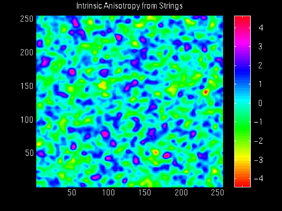
FIG. 1.: A ten degree square patch of the microwave sky according to the cosmic string theory for structure formation. The colour scale shows the temperature contrast $\delta T/T$ in units of one standard deviation. The numbers along the sides of the Figure are grid units. The standard deviation for the string maps, adopting the COBE normalisation of ref. [14], but with a sky rms [18] on $10^{o}$ of 35 $\mu K$, is $\sigma=2.5\times 10^{-5}$.

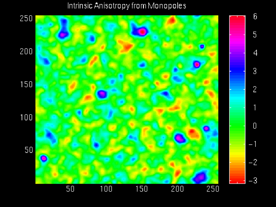
FIG. 2.: As in Figure 1, but for global monopoles. The standard deviation for the monopole maps, adopting the COBE normalisation of ref. [11], but with a sky rms [18] on $10^{o}$ of 35 $\mu K$, is $\sigma=2.2\times 10^{-5}$.

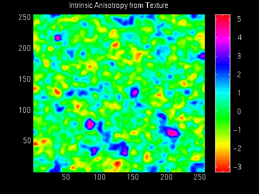
FIG. 3.: As in Figure 1, but for texture. The standard deviation for the texture maps, adopting the COBE normalisation of ref. [11], but with a sky rms [18] on $10^{o}$ of 35 $\mu K$, is $\sigma=2.3\times 10^{-5}$.

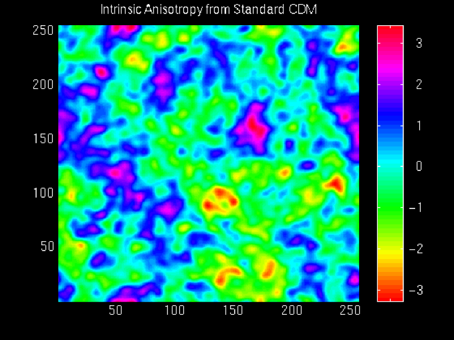
FIG. 4.: As in Figure 1, but for standard inflation.

FIG. 5.: The angular power spectrum of intrinsic CMB anisotropies in the cosmic defect theories. The anisotropy is expanded in spherical harmonics, $(\delta T/T)=\Sigma a_{lm}Y_{lm}(\theta,\phi)$, and $C_{l}$ is defined as $<|a_{lm}|^{2}>$. The solid red, green and blue lines, linking crosses, triangles and boxes respectively, show the numerically determined power spectra for cosmic strings, global monopoles and textures, when the theories are normalised to COBE according to the results of refs. [11] and [14]. The dashed lines show the contribution from the intrinsic temperature term $(\delta T/T)_{i}$ alone (see text). The solid black curve shows the results for the texture model of reference [5], scaled down by a factor of 0.6 after normalising to COBE at low $l$. The dashed line shows the full $C_{l}$ spectrum for the ‘standard’ inflationary theory.

FIG. 6.: The differential number of maxima and minima of the temperature maps in a given range of $(\delta T/T)=\nu\sigma$, measured in units of the standard deviation $\sigma$. The solid red, green and blue lines, linking crosses, triangles and boxes respectively, show the results for maxima for cosmic strings, monopoles and textures. The dashed lines show the number of minima plotted against the negative of the height in the same theories. In a Gaussian theory, the curves for maxima and minima are identical, and are computable from the power spectra $C_{l}$ [21]. The curves shown for minima resemble those for a Gaussian random field, whilst the curves for maxima are clearly nonGaussian, most markedly so for monopoles and textures.

REFERENCES

- [1] T.W.B. Kibble, J. Phys. A9, 1387-1398, (1976).
- [2] A. Vilenkin and E.P.S. Shellard, Cosmic Strings and other Topological Defects, Cambridge University Press, 1994.
- [3] N. Turok, Phys. Scr. T36, 135-141 (1991).
- [4] L. Kofman, A. Linde and A.A. Starobinsky, Phys. Rev. Lett. 76, 1011-1014, (1996).
- [5] R. Crittenden and N. Turok, Physical Review Letters 75, 2642 (1995).
- [6] R. Durrer, A. Gangui and M. Sakellariadou, Phys. Rev. Lett. 76, 579 (1996).
- [7] A. Albrecht, D. Coulson, P. Ferreira and J. Magueijo, Phys. Rev. Lett. 76, 1413-1416 (1996); MRAO preprint 1917 (1996), astro-ph 9605047.
- [8] N. Turok, DAMTP preprint, astro-ph 9604172 (1996).
- [9] W. Hu, D.N. Spergel and M. White, IAS preprint (1996) astro-ph/9605193.
- [10] D.P. Bennett and S.H. Rhie, Ap. J. 406, L7-L10, (1993).
- [11] U. Pen, D. Spergel and N. Turok, Phys. Rev. D 49, 692-729, (1994).
- [12] R. Durrer and Z.H. Zhou, Phys. Rev. D 53, 5394-5410,(1996).
- [13] B. Allen, R. Caldwell, E.P.S. Shellard, A. Stebbins and S. Veeraraghavan, Phys. Rev. Lett., submitted (1996).
- [14] D. Coulson, P. Ferreira, P. Graham and N. Turok, Nature 368, 27-31 (1994).
- [15] R.K. Sachs and A.M. Wolfe, Ap. J. 147, 73-95 (1967).
- [16] S. Veeraraghavan and A. Stebbins, Ap. J. 365, 37-66, (1990)
- [17] J. Magueijo, A. Albrecht, D. Coulson and P. Ferreira, Phys. Rev. Lett. 76, 2617-2620, (1996).
- [18] I thank K. Gorski for help in this.
- [19] R. Battye, Imperial College preprint, Phys. Rev. D, Rapid Communications, submitted (1996).
- [20] F. Bouchet, D.P. Bennett and A. Stebbins, Nature 335, 410-414, (1988).
- [21] J.R. Bond and G. Efstathiou, Mon. Not. Roy. Ast. Soc., 226, 655-687, (1987).