X-rays from superbubbles in the Large Magellanic Cloud IV:
The Blowout Structure of N44

Abstract

We have used optical echelle spectra along with ROSAT and ASCA X-ray spectra to test the hypothesis that the southern portion of the N44 X-ray bright region is the result of a blowout structure. Three pieces of evidence now support this conclusion. First, the filamentary optical morphology corresponding with the location of the X-ray bright South Bar suggests the blowout description (Chu et al. 1993). Second, optical echelle spectra show evidence of high velocity ($\sim$90 km sec^-1) gas in the region of the blowout. Third, X-ray spectral fits show a lower temperature for the South Bar than the main superbubble region of Shell 1. Such a blowout can affect the evolution of the superbubble and explain some of the discrepancy discussed by Oey & Massey (1995) between the observed shell diameter and the diameter predicted on the basis of the stellar content and Weaver et al.’s (1977) pressure-driven bubble model.

1 Introduction

Interactions between massive stars and the interstellar medium (ISM) are among the dominant mechanisms involved in the chemical and dynamical evolution of galaxies. Massive stars deposit thermal and kinetic energy into the ISM through their energetic winds and eventual supernova explosions. One incarnation of these interactions is the “superbubble,” a large ($\sim$100-200 pc diameter), roughly spherical interstellar shell around one or more OB associations. A superbubble shell consists of interstellar material swept up by the stellar winds and supernova ejecta. The shell interior contains hot (10⁶ K), shocked wind and ejecta with density of $\sim 0.01$ cm^-3 surrounded by the cooler, denser gas of the shell (Castor, McCray, & Weaver 1975; Weaver et al. 1977).

A large number of superbubbles have been identified in Local Group galaxies. The Large Magellanic Cloud (LMC) is a nearly ideal laboratory in which to study the detailed physics of these interstellar structures, as the LMC has a low foreground interstellar extinction and a small inclination angle of $\sim$40^∘ (Feast 1991), minimizing confusion along the line-of-sight. At the LMC distance of 50 kpc, 1^′ corresponds to 15 pc, allowing us to study the gas portions of these structures in great detail with a variety of instruments, as well as to resolve the bulk of the individual massive stars with ground-based telescopes. Dozens of superbubbles are known in the LMC, giving many examples for study.

N44 is among the most luminous H ii complexes in the LMC, and consists of three OB associations and several regions of optical nebulosity (Henize 1956; Lucke & Hodge 1970). A variety of H$\alpha$-bright structures are seen in N44, and identifications of the components, both bright knots and large filamentary arcs, have been made by Henize (1956) with labels N44 A – N and Davies, Elliott, & Meaburn (1976) with labels DEM L140 – 170. Figure 1a shows an H$\alpha$ CCD image of the region with the major emission regions marked. Meaburn & Laspias (1991) detected the expansion of the two of the large shells, DEM L140 and DEM L152, confirming their description as superbubbles.

Diffuse X-ray emission from various portions of the N44 region was detected by the Einstein Observatory (Chu & Mac Low 1990; Wang & Helfand 1991). Observations of the region with ROSAT (Chu et al. 1993, hereafter C93) allowed for a more detailed comparison between the X-ray and H$\alpha$ morphologies, and showed several distinct features. C93 used the X-ray morphology to define five regions of particular interest: Shells 1 – 3, the South Bar, and the North Diffuse region. Among the three brightest regions, Shell 1 was identified as an X-ray-bright superbubble, the South Bar was suggested to be a “blowout structure” from the superbubble, and Shell 3 was identified as a previously unknown supernova remnant (SNR). These three bright X-ray features are marked in Figure 2a, a ROSAT Position Sensitive Proportional Counter (PSPC) image overlaid with H$\alpha$ contours. The North Diffuse region is outside of the bounds of this picture and Shell 2 is not shown and will not be discussed further in this paper. Shell 1 corresponds primarily with the interior of the optical shell DEM L152.

The stellar content of DEM L152 has recently been discussed by Oey & Massey (1995 – hereafter OM95), who make model comparisons between the observed expansion velocities and the expected energy input from the stellar winds. Two important results are drawn from their study. First, the stellar content interior to the shell is generally older than the population immediately exterior to the shell ($\sim 10$ Myr vs. $<$5 Myr), suggestive of sequential star formation. Second, their superbubble evolution models, adopting stellar wind and supernova energy inputs implied by realistic stellar contents, over-predict the shell diameter. Several possible reasons for this size discrepancy are given by OM95; however, we believe that part of the discrepancy may be caused by significant energy/pressure lost via the blowout shown in C93.

In this paper, we have combined newly-obtained H$\alpha$ CCD images, high-resolution echelle spectroscopy and ASCA X-ray observations, along with the existing ROSAT observations to test the hypothesis that the South Bar is the result of a blowout.

2 Optical Echelle Spectra

We have used optical spectroscopy to explore the velocity field in the vicinity of the proposed blowout region of the X-ray South Bar. We obtained high-dispersion spectra at the Cerro Tololo Inter-American Observatory (CTIO) using the echelle spectrograph with the long-focus red camera on the 4m telescope. We used the instrument as a single-order, long-slit spectrograph by inserting a post-slit interference filter and replacing the cross-dispersing grating with a flat mirror so that a single echelle order around H$\alpha$ and [N II] $\lambda\lambda$6548 Å, 6583 Å could be imaged over the entire slit. The 79 l/mm grating was used for these observations, and the data were recorded with a Tek 2048$\times$2048 CCD using Arcon 3.6 read-out. With a pixel size of 24$\mu$m pixel^-1, this CCD provided a sampling of $\sim$0.082 Å (3.75 km s^-1) along the dispersion and 0^′′.267 on the sky. Spectral coverage was effectively limited by the bandwidth of the interference filter to 125 Å. Coverage along the slit was 220^′′, including an unvignetted field of $\sim$2^′.5 The instrumental profile, as measured from Th-Ar calibration lamp lines, was 16.1 $\pm$ 0.8 km s^-1 FWHM. The ranges include variations in the mean focus and variations in the focus over a single spectrum. Spatial resolution was determined by the seeing, which was $\sim$1^′′.

The data were bias subtracted at the telescope. Flat-fielding, wavelength calibration, distortion correction, and cosmic ray removal were performed using standard IRAF routines. Wavelength calibration and curvature correction were performed using Th-Ar lamp exposures taken in the beginning of each night. To eliminate velocity errors due to flexure in the spectrograph, the absolute wavelength scale in each spectrum was referenced to the telluric H$\alpha$ airglow feature.

Figure 1 shows the echelle spectrum along with our recent H$\alpha$ CCD image. The CCD image was taken at the Curtis Schmidt telescope at CTIO. This image, along with several other filter images, was taken on February 18, 1994, using the Thompson 1024$\times$1024 CCD. With this setup, the CCD has 1.^′′835 pixels, giving a field of view of 31.^′3. Further details of the Curtis Schmidt observations can be found in Smith et al. (1994). The location of the echelle slit used for the spectrum is indicated on the CCD image. The star labeled “Star 1” shows up clearly at the center of the spectrum. Several cuts in the velocity direction are plotted below the spectrum, and the heliocentric velocity scale is given to the left. The most important feature in this spectrum is the variation in the range of velocities seen. The regions to the east of Star 1 have only a small range of velocities, roughly $-30$ to $+40$ km sec^-1, while to the west, there is clear evidence of significantly blue-shifted material, with velocity offsets up to $\sim-90$ km s^-1. The region with this high-velocity feature coincides with the brightest part of the X-ray South Bar. Also in this area, optical filaments can be seen which extend away from the main optical shell of DEM L152. The high-velocity feature is not detected elsewhere in N44 (Meaburn & Laspias 1991; Hunter 1994), except at another position within the X-ray South Bar (Figure 15 of Hunter 1994). Therefore, the high-velocity gas lends further support to the blowout nature of this region.

3 X-ray Observations

If the South Bar is indeed a blowout structure, with the gas escaping into a region of lower pressure beyond the superbubble shell, it is expected that the temperature of the hot escaping gas should drop as it undergoes adiabatic expansion. To test this hypothesis, we have used X-ray observations from both the ROSAT and ASCA X-ray observatories to compare the temperatures in Shell 1 and the South Bar.

The ROSAT PSPC observations have been discussed in some detail in C93. We present here a brief summary: The observations were performed March 7 – 9, 1992, and are archived under observation number RP500093. For these observations, N44 was centered in the PSPC, where the angular resolution was $\sim$30^′′. The PSPC is sensitive in the energy range of 0.1 – 2.4 keV and has an energy resolution of $\sim$43% at 1 keV. The total effective exposure time was 8871 seconds.

Our ASCA observations were performed March 1, 1995. The ASCA observatory has been discussed by Tanaka et al. (1994). Briefly, the satellite carries four imaging thin-foil grazing incidence X-ray telescopes. Two of the telescopes are focused on solid-state CCD imaging spectrometers, called SIS 0 and SIS 1. The other two telescopes use gas imaging spectrometers (GIS) as the detectors. In this paper, we have only used the SIS data because of the low sensitivity of the GIS for energies below $\sim$1 keV, where our objects are the brightest, and the substantially lower energy resolution compared with the SIS. The SIS detectors have an energy resolution of $\sim$2% at 6 keV and cover the energy range 0.4 – 10 keV, with reduced throughput near the ends of the band. The spatial resolution is poor compared to the ROSAT PSPC, with a narrow core of $\sim$1^′ diameter and a half-power radius of 3^′. Both of the SIS detectors are composed of 4 separate CCDs. Not all CCDs must be run for a given observation, and the presence of “hot” and “flickering” pixels, which fill the telemetry with false signals, have made it necessary to use only a subset of each detector for many observations.

Because of the telemetry limitations, our observations were performed in two-CCD mode, with the South Bar placed at the standard point source location, near the center of the focal plane on SIS0, chip 1 (SIS1 chip 3; see Figure 2b). The observations were performed in faint mode when allowed by the telemetry, and converted to bright mode on the ground for analysis. Using the standard processing software (ascascreen & ftools), we removed bad time periods using the following selection criteria: aspect deviation $<$0.01^∘, angle to bright earth $>$20^∘, elevation $>$10^∘, minimum cutoff rigidity of 6, PIXL rejection of 75. We also removed hot and flickering pixels. After screening, a total of 32,964 sec of usable data remained. We included high, medium, and low bit rate data. Although low bit rate data have been seen to have difficulties in the past, we did not reject them as they constituted $<$1% of our total integration time.

We extracted spectra from the ROSAT and ASCA data using regions which were designed to be as similar as possible to those used in C93. The background was chosen in a different location because the region used by C93 lies outside of the ASCA SIS field of view. The background regions were chosen to exclude point sources and obvious diffuse emission which would contaminate the spectra. The background was taken from a source-free region on chip 0 of SIS0 (chip 2 of SIS1) because there was no region on chip 1 of SIS0 (chip 3 of SIS1) large enough to make a useful measurement. A comparison between a small source free region on chip 1 of SIS0 (chip 3 of SIS1) showed no significant difference with the background we have used. It was necessary to use a local background region in the field because much of the background is contributed by diffuse emission from the LMC itself, in addition to the usual sources of background, such as charged particles, scattered solar light, and cosmic X-ray background. A comparison with the archive background fields shows significant excess emission in the local background field: 0.029 cts sec^-1 for the local background vs 0.018 for the same region of the chip in the archive background field.

For the ASCA data, spectra were extracted from both SIS0 and SIS1. The datasets from both SIS telescopes and the PSPC cannot be simply combined directly (i.e., added together) as the three telescopes have distinct response matrices. Instead, the three spectra were fit jointly to the same models using XSPEC. The normalizations were allowed to fit separately to allow for differences in spatial and spectral resolution. Spectral bins for all three instruments were add together in order to give sufficient counts in each spectral bin that the $\chi^{2}$ statistics would be valid. Optically thin thermal spectra from Raymond & Smith (1977, hereafter RS) and Mewe-Kaastra (Mewe et al. 1985; Kaastra 1992, hereafter MEKA) were used. The abundances of all elements except Fe were set to 30%, consistent with the LMC abundances. Because of some discrepancies in certain Fe line ratios, we allowed the Fe abundance to float to the best fit value, and fixed it at that value to determine the temperature confidence contours. In all fits, the Fe abundances were in the range 1.5% to 7.9% solar, improving the fit substantially over models with the Fe abundance set to 30%. We also experimented with letting other elemental abundances float, but no single element improved the fits substantially. We found that both RS and MEKA models with low Fe abundances were in reasonable agreement with the observed spectra. Derived parameters from the two models were in good agreement with each other.

Figure 3 presents the results of the spectral fits for Shell 1 and the South Bar using the MEKA model. The confidence contours and best-fit spectra are shown. Figure 4 shows the confidence contours and best-fit spectra for Shell 3. The contours suggest that the expected temperature difference between Shell 1 and the South Bar is present: The blowout region (South Bar) has a 99% confidence range for the temperature of 0.29 – 0.49 keV, while the main superbubble (Shell 1) has a 99% confidence range of 0.49 – 0.57 keV, with no overlap of the 99% confidence contours between the two fits. The supernova remnant proposed by C93, Shell 3, does not show a significantly higher temperature as previously claimed – the 99% confidence interval is 0.24 – 0.46 keV. However, this does not refute the identification of this structure with an SNR, and is perhaps more consistent with the observed size of the structure (30 pc) and correspondingly large estimated age ($\sim$1.8 $\times$ 10⁴ yr) reported by C93. The South Bar and Shell 1 have a low absorption, $\sim$10²¹ cm^-2, consistent with the optical and radio measurements of the hydrogen column density (see discussion in C93). The best fit absorption for Shell 3 is 3.8 $\times$ 10²¹ cm^-2. Although the error contour for Shell 3 does not constrain the extinction strongly (1.2 – 6.5 $\times$ 10²¹ cm^-2), it is worthwhile to note that the somewhat higher extinction of Shell 3, compared with Shell 1 and the South Bar is not unreasonable given the presence of faint dust lanes visible across Shell 3 in the H$\alpha$ images.

While these measurements appear to show quite a strong difference in the temperatures of the South Bar and Shell 1, we caution the reader that the confidence contours do not completely describe the true errors involved. In particular the fact that, without allowing the Fe abundance to float, the model spectra deviate systematically from the observed spectra is a point for concern. The problem of poorly-fitting Fe lines has been noted already and blamed on errors in the atomic physics (see e.g., Fabian et al. 1994; Liedahl et al. 1995). Several groups are currently working on updated model calculations incorporating newer atomic data in an effort to improve the situation. Nonetheless, even without such improved models, the relative temperatures of the South Bar and Shell 1 determined with the MEKA and RS models are quite believable. One particular concern of the fits presented here is that there can be a small correlation between the Fe abundance for a fit and the temperature. To show the effect of this correlation, which also plot confidence contours for the fit to the South Bar, keeping the Fe abundance fixed to the best fit value for Shell 1 (gray contours). The significance of the resulting temperature difference is reduced, but still present – now there is overlap between the 99% contours, but the 90% confidence contours do not touch.

4 Discussion

We have used optical echelle spectra along with ROSAT and ASCA X-ray spectra to test the hypothesis that the southern portion of the N44 X-ray bright region is the result of a blowout structure. Three pieces of evidence now support this conclusion. First, the filamentary optical morphology corresponding with the location of the X-ray bright South Bar suggests the blowout description (C93). Second, optical echelle spectra show evidence of high velocity ($\sim$90 km sec^-1) clouds in the region of the blowout. Third, X-ray spectral fits show a lower temperature for the South Bar than the main superbubble region of Shell 1. If the South Bar were the result of escaping gas expanding adiabatically into the surrounding region of lower pressure gas, the temperature would be expected to drop, as is observed. The combination of the optical and X-ray morphology, the high velocity gas seen in the echelle spectra, and these tentative X-ray temperature determinations give strong support to the interpretation of this structure of the South Bar as a blowout from the main shell of the superbubble as suggested by C93.

Such a blowout may explain the discrepancies discussed by OM95 between the observed shell diameter and the diameter predicted on the basis of the stellar content and Weaver et al.’s (1977) pressure-driven bubble model. Below we will discuss N44’s superbubble energetics and the effects of the blowout.

First we use OM95’s stellar content to estimate the total energy input to Shell 1 of N44. OM95 have derived an age of 10 Myr for the stars within the superbubble and 5 Myr for the stars on the exterior. These ages will be used as references. We have integrated the stellar wind power implied by the stellar content (Figure 11 of OM95), and obtained a total stellar wind energy input of 3.2$\times 10^{51}$ erg over the first 5 Myr, and 3.5$\times 10^{51}$ erg over the first 10 Myr. Apparently, the stellar wind input during the second 5 Myr is only about 10% that of the first 5 Myr. The initial mass function of the stars in N44 implies that 1 – 4 supernovae have occurred in the past 10 Myr. It is likely that supernovae dominate the energy input in the second 5 Myr as each explosion deposits $\sim$10⁵¹ erg. The total energy input from the stellar winds and supernovae is probably in the range of $(4-7)\times 10^{51}$ erg.

We may use the model fits derived from the ASCA SIS and ROSAT PSPC data to determine more accurately the thermal energy in the superbubble interior. Using a log N_H of 21.0 and a kT of 0.55 keV for the superbubble interior, the observed ROSAT flux gives a normalization factor log (N${}_{e}^{2}$V/4$\pi$D²) = 11.05 in cgs units, where N_e is the electron density, V is the X-ray emitting volume, and D is the distance to the LMC (50 kpc). We use the ROSAT flux since the better angular resolution of the PSPC implies that fewer photons are lost due to high-angle scattering. If we assume that the X-ray emitting volume is only 1/2 of the superbubble volume (1.2 $\times$ 10⁵ pc³), we derive an N_e of 0.14 cm^-3, a mass of 194 M_⊙, and a thermal energy of 2$\times$10⁵⁰ erg. If the X-ray emitting volume is only 1/100 of the superbubble volume, because of a small filling fraction, then N_e is increased to 1.0 cm^-3, the mass is reduced to 28 M_⊙, and the thermal energy is reduced to 3$\times$10⁴⁹ erg.

In Weaver et al.’s (1977) pressure-driven wind-blown bubble model, the thermal energy in the hot interior should be about 5/11 of the total stellar wind energy input. We see clearly that the thermal energy derived from our X-ray observations is at least an order of magnitude lower than expected. Assuming the input energy from stellar winds and supernovae is correct, this energy discrepancy can be caused by two effects – energy leakage through the blowout and energy loss via radiation. To test the effect of energy loss via cooling, we note that the cooling timescale is roughly (1/N_e) Myr. For the possible range of N_e values, the cooling timescale would be a few Myr; therefore, we may expect a reduction of the thermal energy by a factor of 2, or a few at most. Another mechanism must account for the rest of the lost energy – one possibility is the blowout.

The amount of energy lost in the blowout can be roughly estimated from the X-ray data. Using the ASCA SIS model fit of the blowout region, log N_H = 21.0 and kT = 0.41 keV, we obtain a normalization factor log (N${}_{e}^{2}$ V / 4$\pi$D²) = 10.85 in cgs units. If we assume that the depth of the X-ray emission is the same as the width, the emitting volume is 4$\times$10⁴ pc³, N_e is 0.13 cm^-3, the thermal energy is 1.0$\times 10^{50}$ erg, and the mass is 133 M_⊙. Note that the X-ray emitting volume could be overestimated by a factor of 2 or more, then the N_e would be a factor of $\sqrt{2}$ higher, and the thermal energy and the mass would be a factor of $\sqrt{2}$ lower. This amount of thermal energy, lost from the superbubble, is similar in magnitude to the thermal energy remaining in the superbubble. The largest uncertainty in this comparison is in the determinations of the emitting volume in the superbubble interior and the blowout. Future High Resolution Imager images may help reduce the uncertainties.

We now examine the thermal energy conversion problem with the blowout and radiative cooling taken into consideration. If we use the low estimates for the electron density, we obtain high estimates for the thermal energies in the superbubble interior and the blowout, 2$\times$10⁵⁰ erg and 1$\times 10^{50}$ erg, but also high estimates for the radiative cooling timescale. Applying the Weaver et al. (1977) model, a total energy input of $(4-7)\times 10^{51}$ erg should have $(2-3)\times 10^{51}$ erg converted to thermal energy in hot gas. The observed thermal energy in the superbubble interior and the blowout together is only 3$\times$10⁵⁰ erg. Even if we assume that 1/2 of the thermal energy has been radiated away (thereby ignoring the high estimate for the cooling timescale), there is still a discrepancy by a factor of 3-5. If we use the high estimates for the density, we would have much lower estimates for the thermal energies, and the discrepancy between observed and expected thermal energies would be even larger. Therefore, we conclude that either the Weaver et al. (1977) model is drastically wrong or the stellar wind energy input must have been over-estimated – we consider the latter to be more likely. A similar conclusion has been reached by García-Segura & Mac Low (1995) in their modeling of the single-star wind-blown bubble NGC 6888; they suggest that stellar wind strengths could have been over-estimated by a factor of $\geq 3$ because stellar winds are clumpy (Moffatt & Robert 1994).

Besides the interior thermal energy, another important reservoir of energy in a superbubble is the expansion of the cool H ii shell. The radius of N44 superbubble is 30 pc, and the expansion velocity is $\sim$40 km s^-1 (Meaburn & Laspias 1991). The density in the shell is unfortunately in the low-density regime for the [S ii] doublet, so it is necessary to follow the procedure outlined by Chu et al. (1995) to derive a rms density from the peak emission measure along the shell rim. The shell thickness is calculated assuming an isothermal shock into a photo-ionized interstellar medium. For a peak emission measure of 1500 – 4000 cm^-6 pc along the rim of the shell (C93), we derive a shell thickness of 0.5 pc, a rms electron density of 12 – 20 cm^-3 in the H ii shell, an ambient density of 0.6 – 1.0 cm^-3, a shell mass of $1,600-2,800$ M_⊙, and a shell kinetic energy of $(2.6-4.4)\times 10^{49}$ erg. This kinetic energy is at least an order of magnitude lower than expected from Weaver et al.’s model assuming a total energy input of $(4-7)\times 10^{51}$ erg. This discrepancy may also be caused by the energy leakage and radiation losses, or by an over-estimate of the stellar wind strengths as discussed above.

The presence of a significant blowout in N44, and the resulting effect on the evolution of the superbubble, has important implications for the hot phase of the ISM and model calculations of superbubbles in galaxies. It is interesting to note that the blowout in N44 is probably within the gaseous disk, instead of into a halo. This assumption is based on the small size of N44 compared with the the scale height of the H i layer, as well as the apparent interaction with the H ii regions to the south. If such blowouts are common in superbubbles in general, theoretical estimates of superbubble sizes will be systematically too large. Such an error would affect model predictions of the ISM distribution in galaxies. It is reasonable to conclude that blowouts of this nature may be common: the blowout discussed in this paper is not trivial to detect, and depended upon the X-ray morphology information. Since N44 is the brightest superbubble in X-rays in the LMC, the blowout in this case is relatively easy to detect. For fainter superbubbles, such blowouts could be common and may simply have gone unnoticed so far. Future work to search for evidence of other, similar blowout structures should be performed.

Figure Captions

Figure 1: top) H$\alpha$ image of the N44 complex with ROSAT X-ray contours overlaid. The major regions of nebulosity are labeled (Henize 1956; DEM). The location of the echelle slit is noted, along with the position of Star 1. bottom) The echelle spectrum, including five representative cuts in the spectral direction. The velocity axis is at the left, showing the heliocentric velocity. In this figure, the contours are draw in pairs, with a white line at a slightly lower value than the black line. This allows the reader to distinguish positive and negative contours.

Figure 2: top) ROSAT X-ray image, with H$\alpha$ contours from our CCD image overlaid. The image has been smoothed with a Gaussian with a FWHM of 45^′′. Four of the features described by Chu et al., (1993) are labeled, and the regions from which spectra were extracted are marked. bottom) ASCA X-ray image, with H$\alpha$ contours overlaid. This image is at the same scale and orientation as (a), and has also been smoothed with a Gaussian with a FWHM of 60^′′. In both figures, the contours are draw in pairs, with a white line at a slightly lower value than the black line. This allows the reader to distinguish positive and negative contours.

Figure 3: Comparison of Shell 1 and South Bar. top) Confidence contours for the spectral fits for Shell 1 (thick, black line) and the South Bar (thick, gray line) in which the Fe abundance is fixed at the best fit value. Also plotted is the confidence contours for the spectral fit for the South Bar, using the best-fit Fe abundance value for Shell 1. The three sets of contours represent 68%, 90%, and 99% confidence levels. bottom) Observed spectra (error bars) and MEKA fits (histograms) for Shell 1 (left) and the South Bar (right). In both of the figures, we have included data from ASCA SIS 0 (thick line), SIS 1 (thin line), and ROSAT PSPC (medium weight line).

Figure 4: left) Confidence contours for the spectral fits for Shell 3 in which the Fe abundance is fixed at the best fit value. The three sets of contours represent 68%, 90%, and 99% confidence levels. right) Observed spectra (error bars) and MEKA fits (histograms) for Shell 3. In this figures, we have included data from ASCA SIS 0 (thick line), SIS 1 (thin line), and ROSAT PSPC (medium weight line).

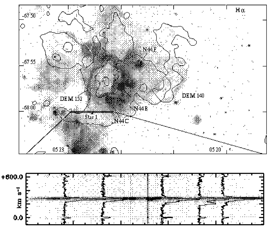
Figure 1:

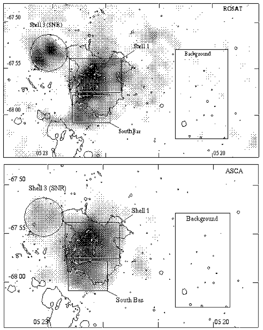
Figure 2:

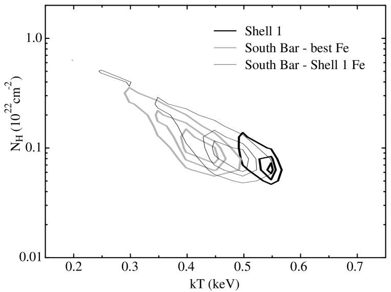
Figure 3:

Figure 4:

References

- (1)
- (2) Castor, J., McCray, R., & Weaver, R. 1975, ApJ 200, L107
- (3) Chu Y.-H., Chang H.-W., Su Y.-L., & Mac Low M.-M. 1995, ApJ 450, 157
- (4) Chu Y.-H. & Mac Low M.-M. 1990, ApJ 365, 510
- (5) Chu Y.-H., Mac Low M.-M., Garcia-Segura G., Wakker B., & Kenicutt R. C. 1993, ApJ 414, 213 (C93)
- (6) Davies R. D., Elliott K. H., & Meaburn J. 1976, MNRAS 81, 89
- (7) Fabian A. C., Arnaud K. A., Bautz M. W., & Tawara Y. 1994, ApJ 436, L63
- (8) Feast M. W. 1991, in IAU Symp. 148, The Magellanic Clouds, ed. R. Haynes & D. Milne (Dordrecht: Kluwer), 1
- (9) García-Segura G. & Mac Low, M.-M. 1995, ApJ 455, 145
- (10) Henize K. G. 1956, ApJS 2, 315
- (11) Kaastra J. S. 1992, An X-ray Spectral Code for Optically Thin Plasmas (SRON-Leiden Report). (MEKA)
- (12) Liedhal D. A., Osterheld A. L., & Goldstein W. H. 1995, ApJ 338, L115
- (13) Lucke P. B. & Hodge P. W. 1970, AJ 75, 171
- (14) Meaburn J. & Laspias N. V. 1991, A&A 245, 635
- (15) Mewe R., Gronenschild E. H. B. M., & van den Oord G. H. J. 1985, A&A 62, 197 (MEKA)
- (16) Oey M. S. & Massey P. 1995, ApJ 452, 216
- (17) Raymond J. C. & Smith B. W. 1977, ApJS 35, 419 (RS)
- (18) Smith R. C., Chu Y.-H., Mac Low M.-M., Oey M. S., & Klein U. 1994, AJ 108, 1266
- (19) Tanaka Y., Inoue H., & Holt S. S. 1994, PASJ 46, L37
- (20) Wang Q. & Helfand D. J. 1991, ApJ 373, 497
- (21) Weaver R., McCray R., Castor J., Shapiro P., & Moore R. 1977, ApJ 218, 377
- (22)