Molecular abundances in the Magellanic Clouds

Abstract

Nine H ii regions of the LMC were mapped in ¹³CO(1–0) and three in ¹²CO(1–0) to study the physical properties of the interstellar medium in the Magellanic Clouds. For N113 the molecular core is found to have a peak position which differs from that of the associated H ii region by 20. Toward this molecular core the ¹²CO and ¹³CO peak $T_{\rm MB}$ line temperatures of 7.3 K and 1.2 K are the highest so far found in the Magellanic Clouds. The molecular concentrations associated with N113, N44BC, N159HW, and N214DE in the LMC and LIRS 36 in the SMC were investigated in a variety of molecular species to study the chemical properties of the interstellar medium. $I$(HCO⁺)/$I$(HCN) and $I$(HCN)/$I$(HNC) intensity ratios as well as lower limits to the $I$(¹³CO)/$I$(C¹⁸O) ratio were derived for the rotational 1–0 transitions. Generally, HCO⁺ is stronger than HCN, and HCN is stronger than HNC. The high relative HCO⁺ intensities are consistent with a high ionization flux from supernovae remnants and young stars, possibly coupled with a large extent of the HCO⁺ emission region. The bulk of the HCN arises from relatively compact dense cloud cores. Warm or shocked gas enhances HCN relative to HNC. From chemical model calculations it is predicted that $I$(HCN)/$I$(HNC) close to one should be obtained with higher angular resolution ($\la$ 30) toward the cloud cores. Comparing virial masses with those obtained from the integrated CO intensity provides an H₂ mass-to-CO luminosity conversion factor of $1.8\times 10^{20}$ mol cm^-2 (${\rm K\,km\,s}^{-1}$)^-1 for N113 and $2.4\times 10^{20}$ mol cm^-2 (${\rm K\,km\,s}^{-1}$)^-1 for N44BC. This is consistent with values derived for the Galactic disk.

1 Introduction

The Large Magellanic Cloud (LMC) and the Small Magellanic Cloud (SMC), the two galaxies closest to the Milky Way, provide unique opportunities to study astrophysical processes (e. g. Westerlund 1991). In regard to the interstellar medium, there are three outstanding properties which motivate detailed investigations: (1) the Magellanic Clouds consist of material characterized by a smaller metallicity than the Milky Way; (2) their UV radiation fields are stronger than in the solar neighborhood; (3) they provide a large number of targets at a well determined distance. The first two properties have far reaching consequences for the astrophysical conditions of the interstellar medium: an absence of dust and extinction in the molecular cloud envelopes results in reduced shielding against the intense UV radiation and decreases the sizes of molecular clouds relative to atomic gas components (e. g. Lequeux et al. 1994). The low metallicities are also expected to have consequences on molecular abundances.

The ESO-SEST Key Programme (e. g. Israel et al. 1993) included observations of the ¹²CO(1–0) and ¹³CO(1–0) spectral lines toward IRAS sources and H ii regions in the LMC and the SMC. With the Australia Telescope Compact Array in Narrabri, Hunt & Whiteoak (1994) discovered a second 4.8 GHz compact radio component in the LMC H ii region N159 (hereafter N159HW), where no H$\alpha$ emission had been found. This detection motivated our search for ¹³CO(1–0) cores offset from the centers of some of the most prominent H ii regions. In order to determine the position of brightest emission in molecular clouds, we thus mapped nine H ii regions in the LMC, which have particularly strong ¹²CO(1–0) and ¹³CO(1–0) line intensities according to the ESO-SEST Key Programme. Toward peaks of three of these sources and N159HW we also made 3 mm multiline studies to elucidate the chemical and physical conditions of the cloud cores.

The SMC is even more metal poor than the Large Magellanic Cloud. Hence a comparison of molecular data from a variety of environments like the inner and outer Galactic disk and the LMC also has to include the SMC. This widens the range of covered metallicities by a factor of 3. In previous studies, the molecular line observations toward the SMC were confined to ¹²CO and ¹³CO transitions (Rubio et al. 1993a,b). We therefore observed LIRS 36, which shows the brightest ¹²CO(1–0) and ¹³CO(1–0) emission peaks observed with the ESO-SEST Key Programme, in a variety of molecular transitions.

Table 1: Positions and velocities for observed objects

Galaxy	Object	$\alpha_{1950}$	$\delta_{1950}$	${v_{\rm LSR}}$
		[${}^{\rm h\ m\ s}$]	[∘  ]	[${\rm km\,s}^{-1}$]
SMC	LIRS 36	0 44 50.5	$-$73 22 33	126.1
LMC	N79	4 52 09.5	$-$69 28 21	233.5
	N83A	4 54 17.0	$-$69 16 23	245.0
	N11	4 55 35.5	$-$66 38 48	279
	N105A	5 10 05.6	$-$68 57 00	241.6
	N113	5 13 40.2	$-$69 25 37	234.8
	N44BC	5 22 10.6	$-$68 00 32	283.0
	N55A	5 32 30.0	$-$66 29 21	290
	N159HW	5 40 04.4	$-$69 46 54	238.3
	N160	5 40 09.0	$-$69 40 13	238.9
	N214DE	5 40 36.3	$-$71 11 30	228.9

Table 2: Summary of observed transitions in $\lambda$ $\approx$ 3 mm range.

Molecule			Frequency		Beamwidth
& Transition			[GHz]		[]
C3H2	$J$=2${}_{1,2}-$10,1		85.	338890	61
HC2	$N$=1–0,       $J$=3/2–1/2	$\left\{\makebox{\rule[-4.30554pt]{0.0pt}{4.30554pt}}\right.$ $F$=2–1 $F$=1–0	87. 316925   87. 328624		60
HCN	$J$=1–0	$\left\{\makebox{\rule[-8.61108pt]{0.0pt}{8.61108pt}}\right.$ $F$=1–1 $F$=2–1 $F$=0–1	88. 630416   88. 631847 88. 633936		59
HCO+	$J$=1–0		89.	188518	58
HNC	$J$=1–0		90.	663543	57
CH3OH	$J$=2–1		96.	741420	54
CS	$J$=2–1		97.	980968	53
C18O	$J$=1–0		109.	782160	47
13CO	$J$=1–0		110.	201353	47
C17O	$J$=1–0		112.	358780	46
CN	$N$=1–0,       $J$=3/2–1/2	$\left\{\makebox{\rule[-8.61108pt]{0.0pt}{8.61108pt}}\right.$ $F$=3/2–1/2 $F$=5/2–3/2 $F$=1/2–1/2	113. 488140 113. 490982 113. 499639		46
12CO	$J$=1–0		115.	271204	45

Figure 1: ¹³CO contour maps observed toward a) N79 (contour levels: 0.30 to 2.30 by 0.40 ${\rm K\,km\,s}^{-1}$, integration between 239 and 252 ${\rm km\,s}^{-1}$ (${v_{\rm LSR}}$)), b) N83A (contour levels: 0.45 to 2.25 by 0.30 ${\rm K\,km\,s}^{-1}$, integration between 239 and 252 ${\rm km\,s}^{-1}$), c) N11 (contour levels: 0.50 to 2.00 by 0.25 ${\rm K\,km\,s}^{-1}$, integration between 274 and 286 ${\rm km\,s}^{-1}$), d) N105A (contour levels: 0.40 to 1.90 by 0.30 ${\rm K\,km\,s}^{-1}$, integration between 237 and 246 ${\rm km\,s}^{-1}$), e) N55A (contour levels: 0.50 to 1.70 by 0.20 ${\rm K\,km\,s}^{-1}$, integration between 282 and 294 ${\rm km\,s}^{-1}$), f) N160 (contour levels: -0.30 to 2.10 by 0.30 ${\rm K\,km\,s}^{-1}$, integration between 231 and 243 ${\rm km\,s}^{-1}$). Typical r.m.s. values are between 0.1 and 0.2 ${\rm K\,km\,s}^{-1}$.

Figure 2: Contour maps of N113 in a) ¹²CO(1–0), where the contour levels are 0 to 50 by 5 ${\rm K\,km\,s}^{-1}$ with the integration between 230 and 242 ${\rm km\,s}^{-1}$ in ${v_{\rm LSR}}$; b) ¹³CO(1–0), where the contour levels are 0.3 to 5.8 by 0.5 ${\rm K\,km\,s}^{-1}$ with the integration between ${v_{\rm LSR}}$ = 231 and 240 ${\rm km\,s}^{-1}$. Typical r.m.s. values are 0.4 and 0.15 ${\rm K\,km\,s}^{-1}$, respectively.

Figure 3: Contour maps of N44BC in a) ¹²CO(1–0), where the contour levels are 0 to 54 by 6 ${\rm K\,km\,s}^{-1}$ with the integration between 276 and 290 ${\rm km\,s}^{-1}$ in ${v_{\rm LSR}}$; b) ¹³CO(1–0), where the contour levels are 0.4 to 7.6 by 1.2 ${\rm K\,km\,s}^{-1}$ with the integration between ${v_{\rm LSR}}$ = 276 and 290 ${\rm km\,s}^{-1}$. Typical r.m.s. values are 0.4 and 0.13 ${\rm K\,km\,s}^{-1}$, respectively.

Figure 4: Contour maps of N214DE in a) ¹²CO(1–0), where the contour levels are 0 to 35 by 5 ${\rm K\,km\,s}^{-1}$ with the integration between 220 and 240 ${\rm km\,s}^{-1}$ in ${v_{\rm LSR}}$; b) ¹³CO(1–0), where the contour levels are 0 to 5 by 1 ${\rm K\,km\,s}^{-1}$ with the integration between ${v_{\rm LSR}}$ = 220 and 240 ${\rm km\,s}^{-1}$. Typical r.m.s. values are 0.7 and 0.23 ${\rm K\,km\,s}^{-1}$, respectively.

2 Observations

Positions and radial velocities of the sources observed are displayed in Table 1. Using the 15-m Swedish-ESO Submillimetre Telescope (SEST) at La Silla, Chile, most of the $\lambda$ $\approx$ 3 mm measurements were carried out in September 1993, May 1994 and January 1995. Frequencies of observed transitions (taken from Lovas 1992) and correspondent antenna beamwidths are summarized in Table 2. A Schottky 3-mm receiver yielded overall system temperatures ($T_{\rm sys}$), including the sky, of order 400 K on a main-beam brightness temperature ($T_{\rm MB}$) scale. $T_{\rm sys}$ was significantly higher only for ¹²CO(1–0), reaching 800 K. In January 1996 a new SIS receiver was employed with $T_{\rm sys}$ $\approx$ 500 K for the $J$=1–0 transitions of ¹²CO and ¹³CO. The backend was an acousto-optical spectrometer with 2000 contiguous channels and a channel separation of 43 kHz (0.11 – 0.15 ${\rm km\,s}^{-1}$ for frequency range 115 – 85 GHz). The observations were carried out in a dual beam-switching mode (switching frequency 6 Hz) with a beam throw of 1140 in azimuth. ¹²CO(1–0) measurements were also carried out in a frequency-switching mode. A comparison of these two sets of data showed consistency in line shapes and intensities, confirming that insignificant emission was present at the reference positions. The on-source integration time of each spectrum varied from 8 minutes for ¹²CO to 260 minutes for HCN toward LIRS 36. All spectral intensities obtained were transformed to a $T_{\rm MB}$ scale, and corrected for a main-beam efficiency 0.74 (Dr. L.B.G. Knee priv. comm.). The pointing accuracy, obtained from measurements of SiO maser sources, was better than 10.

The software package CLASS was used for data reduction. In most cases a linear baseline correction was sufficient. A higher order baseline was occasionally needed for the spectra obtained in the frequency-switching mode, but in all cases the spectral lines were sufficiently narrow so that baseline removal posed no problems.

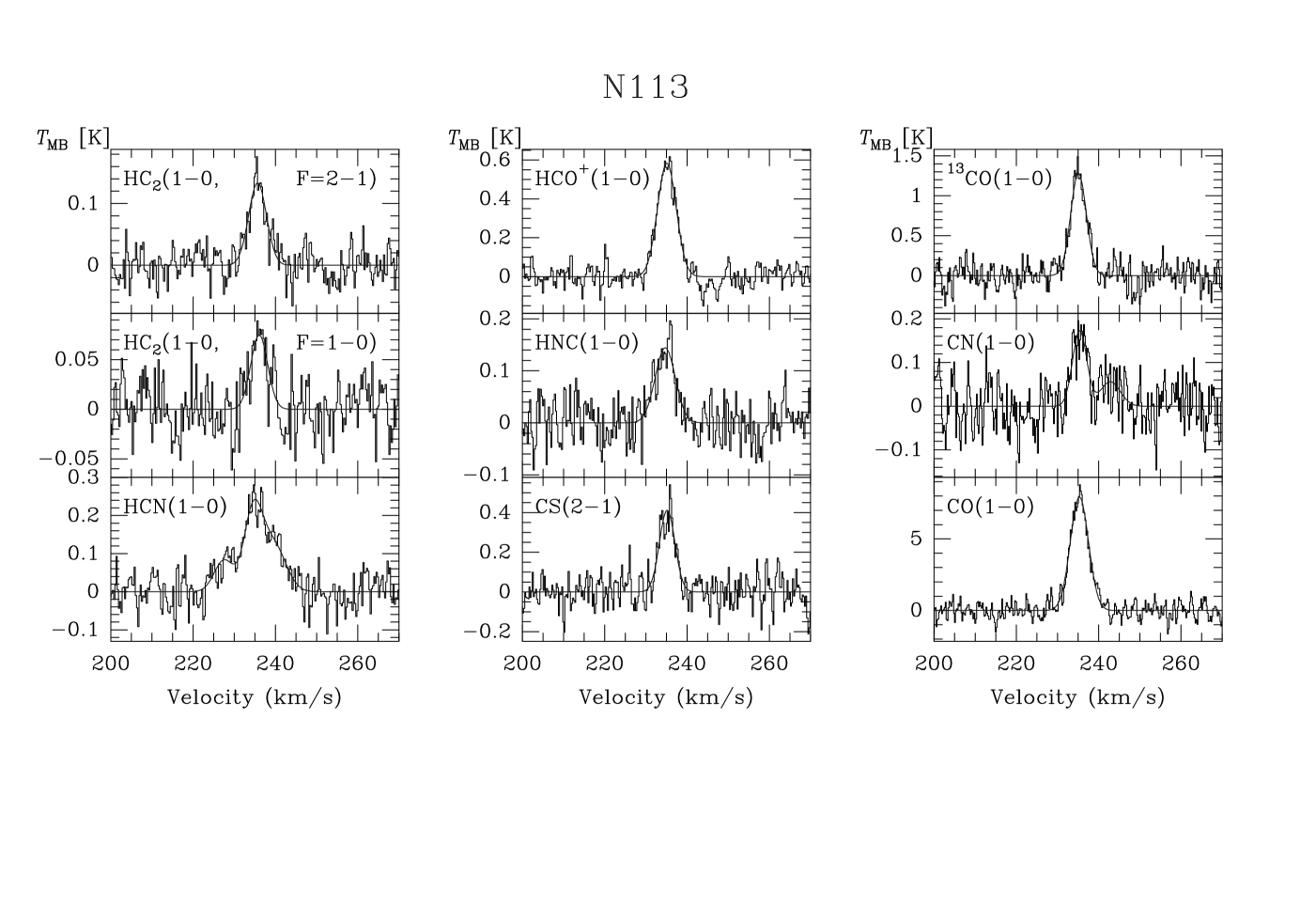
Figure 5: Molecular spectra toward the core of N113

Table 3: Parameters of the Observed Molecular Lines toward the core of N113

Molecule		$T_{\rm MB}$	r.m.s.	${v_{\rm LSR}}$	$\Delta v_{1/2}$	$\int$ $T_{\rm MB}$ d$v$			Velocity Range
& Transition		[K]	[mK]	[${\rm km\,s}^{-1}$]	[${\rm km\,s}^{-1}$]	[${\rm K\,km\,s}^{-1}$]			[${\rm km\,s}^{-1}$]
HC2	$N$=1–0 $J$=3/2–1/2 $\left\{\makebox{\rule[-4.30554pt]{0.0pt}{4.30554pt}}\right.$ $F$=2–1 $F$=1–0	0.133 0.075	27	235.7 236.1	5.1 4.8	0. 716 $\pm$ 0.036 0. 400 $\pm$ 0.034			(230,242) (230,241)
HCN a)	$J$=1–0 $\left\{\makebox{\rule[-8.61108pt]{0.0pt}{8.61108pt}}\right.$ $F$=1–1 $F$=2–1 $F$=0–1	0.124 0.202 0.083	46	234.6	7.2 5.2 5.6	2.	44 $\pm$	0.10	(220,252)
HCO+	$J$=1–0	0.583	53	235.1	5.4	3.	29 $\pm$	0.07	(229,241)
HNC	$J$=1–0	0.144	40	234.7	5.8	0.	867 $\pm$	0.055	(228,241)
CS	$J$=2–1	0.412	79	235.2	4.4	1.	94 $\pm$	0.10	(230,240)
13CO	$J$=1–0	1.28	158	235.1	4.5	6.	06 $\pm$	0.18	(230,241)
CN b)	$N$=1–0 $J$=3/2–1/2 $\left\{\makebox{\rule[-4.30554pt]{0.0pt}{4.30554pt}}\right.$ $F$=3/2–1/2 $F$=5/2–3/2	0.056 0.172	56	235.4	5.7 4.1	0. 319 $\pm$ 0.060 0. 753 $\pm$ 0.053			(231,239) (239,249)
12CO	$J$=1–0	7.92	570	235.3	5.2	44.	1 $\pm$	0.7	(230,242)

1. The three HCN hyperfine transitions ($F$=1–1, $F$=2–1, $F$=0–1) have been resolved by a gaussian fit. While $T_{\rm MB}$ values for each component are given, the total integrated line intensity refers to the entire line.

2. Only $J$=3/2–1/2 transitions of CN($N$=1–0) were covered by the high-resolution AOS backend; two of the hyperfine transitions ($F$=3/2–1/2 and $F$=5/2–3/2) were detected.

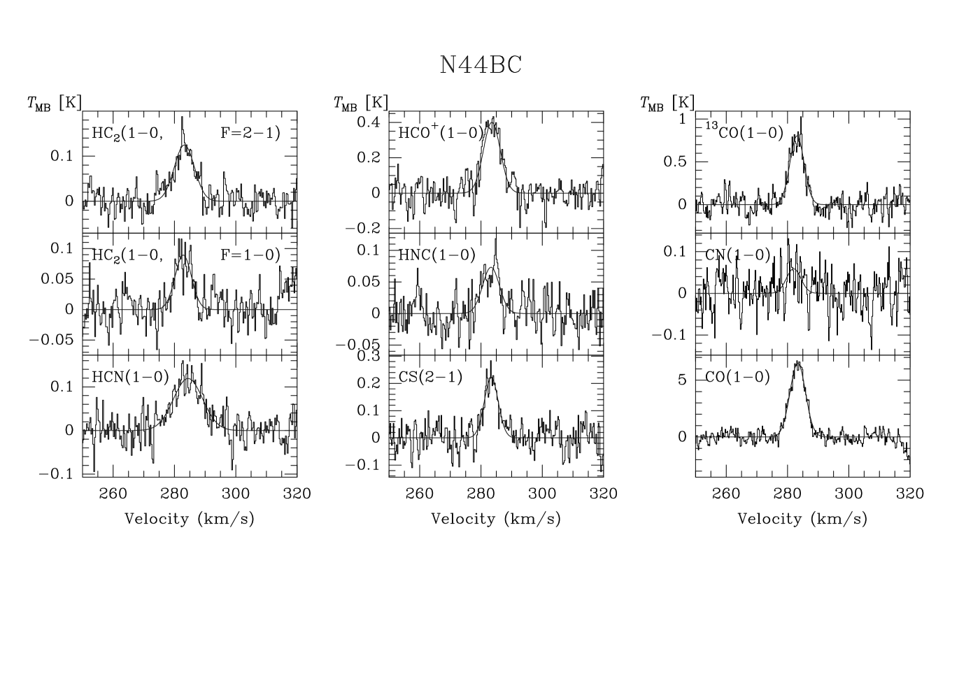
Figure 6: Molecular spectra toward N44BC

Table 4: Parameters of the Observed Molecular Lines toward N44BC

Molecule		$T_{\rm MB}$	r.m.s.	${v_{\rm LSR}}$	$\Delta v_{1/2}$	$\int$ $T_{\rm MB}$ d$v$			Velocity Range
& Transition		[K]	[mK]	[${\rm km\,s}^{-1}$]	[${\rm km\,s}^{-1}$]	[${\rm K\,km\,s}^{-1}$]			[${\rm km\,s}^{-1}$]
HC2	$N$=1–0 $J$=3/2–1/2 $\left\{\makebox{\rule[-4.30554pt]{0.0pt}{4.30554pt}}\right.$ $F$=2–1 $F$=1–0	0.125 0.089	26	283.2 282.9	7.7 6.3	1. 10 $\pm$ 0.04 0. 568 $\pm$ 0.040			(274,292) (275,291)
HCN a)	$J$=1–0	0.119	32	284.4	11.2	1.	36 $\pm$	0.06	(270,298)
HCO+	$J$=1–0	0.400	74	283.6	6.9	3.	06 $\pm$	0.11	(276,290)
HNC	$J$=1–0	0.073	27	283.3	6.5	0.	521 $\pm$	0.039	(276,290)
CS	$J$2–1	0.221	49	283.4	5.4	1.	32 $\pm$	0.07	(276,290)
13CO	$J$=1–0	0.802	112	283.1	5.5	4.	70 $\pm$	0.14	(276,290)
CN b)	$N$=1–0 $J$=3/2–1/2	0.059	47	282.0	5.6	0.	378 $\pm$	0.059	(276,290)
12CO	$J$=1–0	6.50	475	283.3	6.0	40.	2 $\pm$	0.6	(276,290)

1. The frequency of the main transition, HCN(1–0 $F$=2–1), is given. The three hyperfine transitions ($F$=1–1, $F$=2–1, $F$=0–1) remain unresolved. The relatively large spectral linewidth is caused by blending of these components.

2. Only $J$=3/2–1/2 transitions of CN($N$=1–0) were covered by the high-resolution AOS backend; the $F$=5/2–3/2 hyperfine transition was detected.

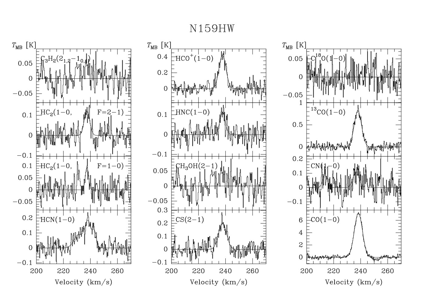
Figure 7: Molecular spectra toward N159HW

Table 5: Parameters of the Observed Molecular Lines toward N159HW

Molecule		$T_{\rm MB}$	r.m.s.	${v_{\rm LSR}}$	$\Delta v_{1/2}$	$\int$ $T_{\rm MB}$ d$v$			Velocity Range
& Transition		[K]	[mK]	[${\rm km\,s}^{-1}$]	[${\rm km\,s}^{-1}$]	[${\rm K\,km\,s}^{-1}$]			[${\rm km\,s}^{-1}$]
C3H2	$J$=2${}_{1,2}-$10,1	$<$ 0.05	32	…	…	$<$ 0.143 c)			(230,245)
HC2	$N$=1–0 $J$=3/2–1/2 $\left\{\makebox{\rule[-4.30554pt]{0.0pt}{4.30554pt}}\right.$ $F$=2–1 $F$=1–0	0.122 0.094	38	237.4 237.4	4.8 2.8	0. 634 $\pm$ 0.058 0. 283 $\pm$ 0.032			(230,245) (235,240)
HCN a)	$J$=1–0 $\left\{\makebox{\rule[-8.61108pt]{0.0pt}{8.61108pt}}\right.$ $F$=1–1 $F$=2–1 $F$=0–1	0.095 0.175 0.087	39	238.2	3.4 5.6 7.9	2.	16 $\pm$	0.08	(224,251)
HCO+	$J$=1–0	0.422	55	237.7	6.1	2.	93 $\pm$	0.08	(230,245)
HNC	$J$=1–0	0.114	38	237.7	4.7	0.	551 $\pm$	0.057	(230,245)
CH3OH	$J$=2–1	$<$ 0.05	32	…	…	$<$ 0.134 c)			(230,245)
CS	$J$=2–1	0.204	44	237.8	6.9	1.	37 $\pm$	0.06	(230,245)
13CO	$J$=1–0	0.814	61	237.9	6.4	5.	42 $\pm$	0.08	(230,245)
CN b)	$N$=1–0 $J$=3/2–1/2 $\left\{\makebox{\rule[-8.61108pt]{0.0pt}{8.61108pt}}\right.$ $F$=3/2–1/2 $F$=5/2–3/2 $F$=1/2–1/2	0.048 0.115 0.076	64	236.9	5.0 4.6 3.6	0. 267 $\pm$ 0.053 0. 512 $\pm$ 0.060 0. 241 $\pm$ 0.053			(242,249) (233,242) (210,217)
12CO	$J$=1–0	7.17	237	238.3	7.0	48.	4 $\pm$	0.3	(228,248)

1. The three HCN hyperfine transitions ($F$=1–1, $F$=2–1, $F$=0–1) have been resolved by a gaussian fit. While $T_{\rm MB}$ values for each component are given, the total integrated line intensity refers to the entire line.

2. Only $J$=3/2–1/2 transitions of CN($N$=1–0) were covered by the high-resolution AOS backend; three of the hyperfine transitions ($F$=3/2–1/2, $F$=5/2–3/2, and $F$=1/2–1/2) were detected.

3. For undetected molecular lines, upper limits of 3 $\times$ r.m.s. are given for $\int$$T_{\rm MB}$ d$v$.

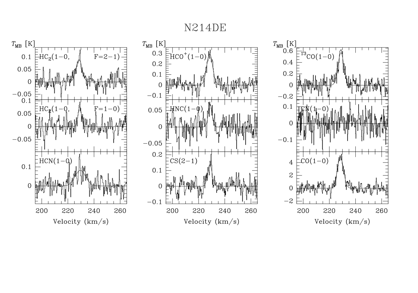
Figure 8: Molecular spectra toward N214DE

Table 6: Parameters of the Observed Molecular Lines toward N214DE

Molecule		$T_{\rm MB}$	r.m.s.	${v_{\rm LSR}}$	$\Delta v_{1/2}$	$\int$ $T_{\rm MB}$ d$v$			Velocity Range
& Transition		[K]	[mK]	[${\rm km\,s}^{-1}$]	[${\rm km\,s}^{-1}$]	[${\rm K\,km\,s}^{-1}$]			[${\rm km\,s}^{-1}$]
HC2	$N$=1–0 $J$=3/2–1/2 $\left\{\makebox{\rule[-4.30554pt]{0.0pt}{4.30554pt}}\right.$ $F$=2–1 $F$=1–0	0.090 0.079	23	228.5 229.1	5.5 3.0	0. 536 $\pm$ 0.033 0. 258 $\pm$ 0.030			(222,235) (224,235)
HCN a)	$J$=1–0	0.082	33	229.5	9.6	0.	831 $\pm$	0.055	(220,239)
HCO+	$J$=1–0	0.294	47	228.4	5.4	1.	75 $\pm$	0.06	(222,235)
HNC	$J$=1–0	0.069	27	228.8	3.5	0.	278 $\pm$	0.037	(222,235)
CS	$J$=2–1	0.138	38	228.6	4.1	0.	621 $\pm$	0.049	(222,235)
13CO	$J$=1–0	0.571	92	228.8	5.3	3.	36 $\pm$	0.11	(222,235)
CN b)	$N$=1–0 $J$=3/2–1/2	$<$ 0.06	59	…	…	$<$ 0.22 c)			(222,235)
12CO	$J$=1–0	4.86	566	228.5	5.5	29.	0 $\pm$	0.7	(222,235)

1. The frequency of the main transition, HCN(1–0 $F$=2–1), is given. The three hyperfine transitions ($F$=1–1, $F$=2–1, $F$=0–1) remain unresolved. The relatively large spectral linewidth is caused by blending of these components.

2. Only $J$=3/2–1/2 transitions of CN($N$=1–0) were covered by the high-resolution AOS backend; the $F$=5/2–3/2 hyperfine transition was detected.

3. For undetected molecular lines, upper limits of 3 $\times$ r.m.s. are given for $\int$$T_{\rm MB}$ d$v$.

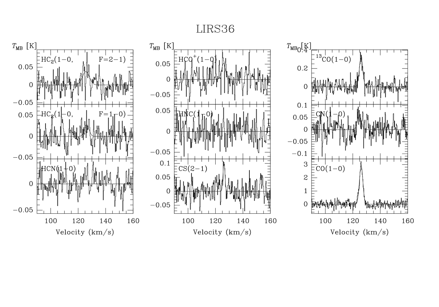
Figure 9: Molecular spectra toward LIRS 36

Table 7: Parameters of the Observed Molecular Lines toward LIRS 36

Molecule		$T_{\rm MB}$	r.m.s.	${v_{\rm LSR}}$	$\Delta v_{1/2}$	$\int$ $T_{\rm MB}$ d$v$		Velocity Range
& Transition		[K]	[mK]	[${\rm km\,s}^{-1}$]	[${\rm km\,s}^{-1}$]	[${\rm K\,km\,s}^{-1}$]		[${\rm km\,s}^{-1}$]
HC2	$N$=1–0 $J$=3/2–1/2 $\left\{\makebox{\rule[-4.30554pt]{0.0pt}{4.30554pt}}\right.$ $F$=2–1 $F$=1–0	0.038 0.027	21	125.6 126.3	6.0 4.0	0.223$\pm$ 0.027 0.093$\pm$ 0.024		(120,131) (122,131)
HCN	$J$=1–0	$<$ 0.02	18	…	…	$<$ 0.064 b)		(121,131)
HCO+	$J$=1–0	0.053	30	125.9	3.3	0.229$\pm$	0.036	(121,131)
HNC	$J$=1–0	$<$ 0.02	26	…	…	$<$ 0.092 b)		(121,131)
CS	$J$=2–1	0.105	30	126.2	1.6	0.276$\pm$	0.035	(121,131)
13CO	$J$=1–0	0.319	57	126.0	3.0	0.923$\pm$	0.061	(121,131)
CN a)	$N$=1–0 $J$=3/2–1/2	0.058	34	124.8	3.4	0.154$\pm$	0.037	(121,131)
12CO	$J$=1–0	2.90	213	126.1	3.0	9.26$\pm$	0.23	(121,131)

1. Only $J$=3/2–1/2 transitions of CN($N$=1–0) were covered by the high-resolution AOS backend; the $F$=5/2–3/2 hyperfine transition was detected.

2. For undetected molecular lines, upper limits of 3 $\times$ r.m.s. are given for $\int$$T_{\rm MB}$ d$v$.

Figure 10: The spectra of the observed carbon monoxide isotopomers CO, ¹³CO, C¹⁸O, and C¹⁷O toward a) N113, b) N44BC, c) N159HW, and d) LIRS 36.

Table 8: Line parameters of carbon monoxide isotopomers

Object	Molecule	$T_{\rm MB}$		r.m.s.	${v_{\rm LSR}}$	$\Delta v_{1/2}$	$\int$ $T_{\rm MB}$ d$v$			Velocity Range
		[K]		[mK]	[${\rm km\,s}^{-1}$]	[${\rm km\,s}^{-1}$]	[${\rm K\,km\,s}^{-1}$]			[${\rm km\,s}^{-1}$]
N113	12CO	7.	92	570	235.3	5.2	32.	4 $\pm$	0.3	(228,242)
	13CO	1.	28	158	235.1	4.5	4.	28 $\pm$	0.07	(228,242)
	C18O	0.	439	12	235.3	3.3	0.	169 $\pm$	0.014	(228,242)
	C17O	$<$ 0.	02	25	…	…	$<$ 0.096 a)			(228,242)
N44BC	12CO	6.	55	475	283.3	6.0	40.	2 $\pm$	0.6	(276,290)
	13CO	0.	802	112	283.1	5.5	4.	70 $\pm$	0.14	(276,290)
	C18O	$<$ 0.	02	25	…	…	$<$ 0.092 a)			(276,290)
	C17O	$<$ 0.	02	22	…	…	$<$ 0.085 a)			(276,290)
N159HW	12CO	7.	17	237	238.3	7.0	52.	4 $\pm$	0.4	(228,248)
	13CO	0.	814	61	237.9	6.4	5.	75 $\pm$	0.08	(230,245)
	C18O	$<$ 0.	03	29	…	…	$<$ 0.116 a)			(230,245)
LIRS 36	12CO	2.	90	213	126.1	3.0	9.	26 $\pm$	0.23	(121,131)
	13CO	0.	319	57	126.0	3.0	0.	923 $\pm$	0.061	(121,131)
	C18O	$<$ 0.	02	34	…	…	$<$ 0.110 a)			(121,131)

1. For undetected CO isotopomers, upper 3 $\sigma$ limits are given for $\int$$T_{\rm MB}$ d$v$.

3 Results

3.1 CO maps toward HII regions in the LMC

¹³CO maps defining the molecular clouds were obtained with a spacing of 30 toward the H ii regions N79, N83A, N11, N105A, N113, N44BC, N55A, N160, and N214DE (20 spacing) in the LMC. In addition, ¹²CO maps with the same spacing were obtained for N113, N44BC, and N214DE (see Table 1). The ¹³CO(1–0) transition is very effective for mapping molecular clouds in the Magellanic Clouds, because the emission providing direct information on column density is strong enough for short integration times. The contour maps are shown in Fig. 1, Fig. 2.b, Fig. 3.b, and Fig. 4.b. In most cases, the offsets of the ¹³CO peak from the H$\alpha$ center are within the pointing error of the SEST. Nevertheless, this is not the case for N113, N214DE, and N160, where right ascension and declination offsets are $\approx$ ($-$10, $-$20), $\approx$ ($-$15, 20), and $\approx$ ($-$35, $-$20), respectively. In N113 the position of the ¹³CO peak is confirmed by a ¹²CO map obtained with a spacing of 20 in the frequency-switching mode. The map shows a compact core which is similar to that observed in ¹³CO (Fig. 2.a). However, contour maps of N44BC and N214DE (Fig. 3 and Fig. 4) show quite different ¹²CO and ¹³CO distributions.

3.2 Multiline study of the Magellanic Clouds

Previously, a comprehensive molecular-line study of an individual Magellanic Cloud H ii region has been made only for N159 (Johansson et al. 1994). While interesting differences between the interstellar medium of the LMC and that of the Galaxy were found, results for one object may not be typical for the entire galaxy. Furthermore, differences in the properties of the rarer molecular species between the LMC and the SMC have not been studied. To further our understanding in these areas, we have observed a variety of $\lambda$=3 mm molecular transitions toward the molecular cores of N113, N44BC, N159HW, and N214DE in the LMC, and LIRS 36 in the SMC. The spectra are shown in Figs. 5 to 9, respectively. The corresponding line parameters of the molecular species, including HC₂, HCN, HCO⁺, HNC, CS, ¹³CO, CN, and ¹²CO, are summarized in Tables 3 – 7 (for the line frequencies and antenna beamwidths, see also Table 2). Toward some of the sources, individual hyperfine components of HCN and CN can be identified. While relative intensities of the CN features are consistent with Local Thermodynamic Equilibrium (LTE) and optically thin line emission, the HCN features show deviations from LTE which are discussed in Sect.4.2.2.

3.3 Observations of CO isotopomers in the Magellanic Clouds

To gain insight into the isotopic composition of the interstellar medium of the Magellanic Clouds, three carbon monoxide isotopomers (¹²CO, ¹³CO, and C¹⁸O) were observed toward the molecular cores of N113, N44BC, N159HW, and LIRS 36, and C¹⁷O was also measured toward N113 and N44BC. The spectra are shown in Fig 10. Table 8 displays the corresponding line parameters. Only upper limits could be obtained in C¹⁸O and C¹⁷O (see also Sect. 4.2.3).

4 Discussion

In the following, cloud stability, $N_{\rm H_{2}}/I_{\rm CO}$ conversion factors, cloud chemistry, and isotope ratios will be discussed for the molecular cores we have observed near prominent H ii regions.

Table 9: Cloud parameters and gravitational stability

Source	$\alpha_{\rm obs}$		$\alpha$		$D$ a)	$\Delta v_{1/2}$	$M_{\rm vir}$		$E_{\rm turb}$		$E_{\rm therm}$	$E_{\rm grav}$	$B_{\rm equi}$
	[]		[]		[pc]	[${\rm km\,s}^{-1}$]	[103 M⊙]		[1042 J]		[1039 J]	[1042 J]	[$\mu$G]
N79	90		78		19	5.3	64		0.	97	24	2.2	55
N83A	75		60		15	6.0	63		1.	2	23	2.8	92
N11	80		66		16	5.3	55		0.	82	20	1.9	65
N105A	80		66		16	7.2	101		2.	8	37	6.5	120
N113	100		89		22	4.5	53		0.	58	20	1.3	34
N44BC	120		111		27	5.6	102		1.	7	38	4.0	43
N55A	75		60		15	6.4	72		1.	6	27	3.7	104
N160	95		84		20	7.3	131		3.	7	48	8.7	98
N214DE	110		100		24	4.7	65		0.	77	24	1.8	34

1. The assumed distance to the LMC is 50 kpc.

4.1 Gravitational stability of the mapped clouds

For the molecular clouds which have been mapped in the ¹³CO(1–0) transition, we can estimate the virial mass, which depends only on the linewidth $\Delta v_{1/2}$ and the (intrinsic) cloud diameter $D$. Assuming a spherical cloud geometry and constant gas density in the clouds, $M_{\rm vir}$ can be obtained from

$$M_{\rm vir}=\frac{5}{8\,\sqrt{3}\,G\,\ln 2}\,D\,(\Delta v_{1/2})^{2}\ ,$$ (1)

where $G$ is the gravitational constant. In terms of astronomically convenient units, this relation becomes

$$M_{\rm vir}\,[{\rm M}_{\odot}]=121\ D\,[{\rm pc}]\ \Delta v_{1/2}\,[{\rm km\,s}^{-1}]\ ,$$ (2)

which is correct to within 10% also for a $1/r$ density profile, and to a factor of two if $n$(H₂) $\propto$ $1/r^{2}$ (e. g. MacLaren et al. 1988). The angular cloud diameter $\alpha$ can be calculated from the observed angular diameter $\alpha_{\rm obs}$ defined by the contour maps with

$$\alpha^{2}=\alpha_{\rm obs}^{2}-HPBW^{2}\ ,$$ (3)

where $HPBW$, the half power beam width, $\approx$ 45 at the frequency of the ¹³CO $J$=1–0 transition.

The stability of the clouds can be evaluated by comparing the turbulent kinetic, thermal, and gravitational energy (e. g. Harju et al. 1992). The turbulent kinetic energy $E_{\rm turb}$ can be estimated from

$$E_{\rm turb}=\frac{3}{2}M_{\rm vir}\sigma^{2}\ .$$ (4)

The one-dimensional turbulent velocity dispersion $\sigma$ is related to the (intrinsic) linewidth by

$$\sigma^{2}=\frac{\Delta v_{\rm int}^{2}}{8\ln 2}-\frac{kT}{m_{{}^{13}{\rm CO}}}\ ,$$ (5)

where $m_{{}^{13}{\rm CO}}$ is the mass of the ¹³CO molecule; $k$ is the Boltzmann constant, and $T$ is the kinetic temperature, assumed to be 30 K (see e. g. Figs. 2a and 5a of Lequeux et al. 1994). The intrinsic line width $\Delta v_{\rm int}$ is derived from the observed line width $\Delta v_{\rm obs}$ and the velocity resolution $\Delta v_{\rm res}$ (0.12 ${\rm km\,s}^{-1}$ for our ¹³CO(1–0) measurement) by:

$$\Delta v_{\rm int}^{2}=\Delta v_{\rm obs}^{2}-\Delta v_{\rm res}^{2}\ ;$$ (6)

or $\Delta v_{\rm int}\approx\Delta v_{\rm obs}$, if $\Delta v_{\rm obs}\gg\Delta v_{\rm res}$.

The thermal energy can be estimated from

$$E_{\rm therm}=\frac{3}{2}NkT\ ,$$ (7)

where $N$ is the total number of H₂ molecules. An upper limit for $N$ can be derived from $N$ = $M_{\rm vir}$/$m_{{\rm H}_{2}}$.

Assuming a homogeneous sphere, the gravitational energy can be expressed as:

$$E_{\rm grav}=\frac{6}{5}\,G\,\frac{M_{\rm vir}^{2}}{D}\ .$$ (8)

The cloud parameters of most of the mapped H ii regions are displayed in Table 9. The gravitational energy is larger than the turbulent kinetic energy and much larger than the upper limit of thermal energy, i. e., $E_{\rm grav}$ $>$ $E_{\rm turb}$ $\gg$ $E_{\rm therm}$. Thus all listed H ii regions seem to be gravitationally unstable. Taking the magnetic energy density $B^{2}/8\pi$ and assuming a uniform magnetic field strength, the magnetic fields required for cloud equilibrium are also given in Table 9. While the results can only be judged to be order of magnitude estimates, it is interesting to see that the calculated magnetic field strengths of several 10 to 120 $\mu$G are slightly larger than the observed magnetic fields in star-forming regions which only refer to the large scale magnetic component parallel to the line of sight (for a summary, see e. g. Fiebig & Güsten 1989; Heiles et al. 1993; Vallée 1995).

For the observed H ii regions the virial masses have been obtained and the gravitational stability has been checked (see Sect. 4.1 and Table 9). Since the ¹²CO(1–0) emission has also been measured toward N113 and N44BC, the H₂ mass-to-CO luminosity conversion factor can be derived with

$$M_{\rm gas}=1.36\,[N_{\rm H_{2}}/I_{\rm CO}]\,m_{\rm H_{2}}\,\sum_{i=1}^{n}\frac{I_{u,i}+I_{l,i}}{2}\,A_{i}\ ,$$ (9)

where 1.36 is the correction to include helium and metals (likely an overestimate but consistent with the value taken in other studies), $m_{\rm H_{2}}$ is the mass of an H₂ molecule, $I_{u,i}$ and $I_{l,i}$ are the integrated intensities of the upper and lower contours confining the area $A_{i}$ (in cm^-2; $n$: number of contours). $X=[N_{\rm H_{2}}/I_{\rm CO}]$ is the conversion factor between integrated ¹²CO $J$=1–0 intensity (in ${\rm K\,km\,s}^{-1}$) and H₂ column density (in cm^-2). For our Galactic disk $X=2.3\times 10^{20}$ mol cm^-2  (${\rm K\,km\,s}^{-1}$)^-1 is standard (Strong et al. 1988). This conversion factor was based on the CO survey by Dame et al. (1987). A re-evaluation of the calibration scheme at the Columbia telescopes (Bronfman et al. 1988) has shown that the CO intensity scale was too low by 22%, thus yielding a conversion factor $X_{\rm Gal}=1.9\times 10^{20}$ mol cm^-2 (${\rm K\,km\,s}^{-1}$)^-1. In the LMC $X_{\rm LMC}\approx 6\,X_{\rm Gal}$ was determined by Cohen et al. (1988). Assuming $M_{\rm gas}$ = $M_{\rm vir}$ we get conversion factors of $X_{\rm N113}=1.8\times 10^{20}$ mol cm^-2 (${\rm K\,km\,s}^{-1}$)^-1 and $X_{\rm N44BC}=2.4\times 10^{20}$ mol cm^-2 (${\rm K\,km\,s}^{-1}$)^-1, which are smaller than the value from Cohen et al. (1988), but close to that in the Galactic disk and that determined by Garay et al. (1993) for the 30 Doradus halo where a value of $2.8\times 10^{20}$ mol cm^-2 (${\rm K\,km\,s}^{-1}$)^-1 was determined. For the SMC Rubio et al. (1993b) found with $X_{\rm SMC}=9\times 10^{20}$  ($R$/10 pc)^0.7 mol cm^-2 (${\rm K\,km\,s}^{-1}$)^-1 a dependence on linear scale length (i. e., beam radius). It seems that the large H₂ mass-to-CO luminosity conversion factor determined by Cohen et al. (1988) for the LMC is caused by a similar scale length dependence. This can be explained by the fact that the molecular clouds are, in general, smaller than the beam size and that the interclump gas is mainly in an atomic phase, not contributing to the integrated CO emission. For compact molecular hot spots in the LMC, the conversion factor appears to be close to the Galactic disk value, in good agreement with the result of Johansson (1991).

4.2 Molecular intensity ratios

Table 10: Integrated $J$=1–0 or $N$=1–0 intensity ratios in the observed H ii regions, in Galactic molecular clouds and in some external galaxies. For IC 443 and W49N, we give abundance ratios. ^a)

Sources	$\frac{\hbox{HCO${}^{+}$}}{\hbox{HCN}}$		$\frac{\hbox{HCN}}{\hbox{HNC}}$		$\frac{\hbox{CN}}{\hbox{HCN}}$		$\frac{\hbox{HC${}_{2}$}}{\hbox{HCN}}$		$\frac{\hbox{CS}}{\hbox{CN}}$		$\frac{\hbox{${}^{12}$CO}}{\hbox{${}^{13}$CO}}$		$\frac{\hbox{${}^{13}$CO}}{\hbox{C${}^{18}$O}}$
N113	1.	35	2.	82	0.	44	0.	46	1.	81	7.	28	36
N44BC	2.	25	2.	61	0.	28	1.	22	3.	50	8.	56	$>$48
N159HW	1.	36	3.	90	0.	52	0.	42	1.	26	9.	12	$>$49
N214DE	2.	10	2.	99	$<$0.	26	0.	96	$>$2.	89	8.	64	…
LIRS 36	$>$3.	59	…		$>$2.	60	$>$5.	5	1.	66	10.	0	$>$8
N159 b)	2.	21	2.	97	0.	48	…		1.	75	8.	31	34
S138 b)	0.	67	3.	75	…		…		…		5.	59	10
M17SW c)	0.	16	1.	9	$\ll$ 1		…		…		4.	9	8	.3
IRC+10216 d)	…		8.	24	1.	24	…		0.	36	10.	8	…
IC 443 e)	1.	2	7.	0	1.	7	…		0.	5	…		…
W49N f)	1.	0	6.	0	0.	5	$>$25.	0	2.	0	…		…
NGC 253	0.	81 g)	1.	3 h)	1.	5 g)	0.	20 i)	0.	51 j)	16.	6 k)	4	.9 l)
IC 342	0.	51 m)	3.	3 h)	0.	79 n)	…		0.	32 o)	11.	1 k)	3	.9 l)
M 82	2.	1 p)	2.	0 h)	1.	4 n)	0.	46 q)	0.	68 o)	15.	9 k)	4	.5 l)
NGC 4945	0.	93 r)	2.	03 r)	1.	48 s)	0.	45 r)	0.	35 r)	14.	4 s)	2	.9 s)

1. Transitions are $J$=1–0 or $N$=1–0 for all molecular species except for CS. For CS, $J$=2–1 intensities were taken. CN line intensities refer to detected $N$=1–0 hyperfine components.

2. Johansson et al. (1994).

3. Baudry et al. (1980), Lada (1976), and Turner & Thaddeus (1977).

4. Nyman et al. (1993).

5. Ziurys et al. (1989).

6. Nyman & Millar (1989).

7. Henkel et al. (1993).

8. Hüttemeister et al. (1995).

9. Israel (1992).

10. CS data from Mauersberger & Henkel (1989), CN data from Henkel et al. (1993).

11. Sage & Isbell (1991).

12. Sage et al. (1991).

13. Nguyen-Q-Rieu et al. (1992).

14. CN data from Henkel et al. (1988), HCN data from Nguyen-Q-Rieu et al. (1992).

15. CS data from Mauersberger & Henkel (1989), CN data from Henkel et al. (1988).

16. Nguyen-Q-Rieu et al. (1989).

17. HC₂ data from Henkel et al. (1988), HCN data from Nguyen-Q-Rieu et al. (1989).

18. Henkel et al. (1990).

19. Henkel et al. (1994).

In Table 10 we present the observed integrated line intensity ratios for the LMC and the SMC. A comparison of these ratios with those from Johansson et al. (1994) for N159, Galactic H ii regions, the shocked molecular gas associated with the supernova remnant, IC 443, the diffuse absorbing gas toward W49N, and a sample of prominent nearby galaxies is also displayed. Most ratios from the sample of Magellanic Cloud sources show self-consistency but indicate significant differences when compared with other classes of objects.

In analyzing molecular line intensities and line shapes, it is often difficult to disentangle abundance variations from changes in excitation conditions. There are, however, ways to circumvent the problem. By observing molecular species with similar excitation properties (i. e. similar electric dipole moments and rotational constants) but with different chemical properties, changes in both chemical and physical conditions may be identified assuming common excitation properties. A good choice is a combined study of HCN, HCO⁺, and HNC in their ground rotational $J$=1–0 transitions. While optical depths cannot be directly determined for most of these species due to a lack of hyperfine splitting, relative intensities provide qualitative information on relative abundances. ¹²CO, ¹³CO, and C¹⁸O intensity ratios are also important for an estimate of ¹²CO opacities and to constrain ¹³CO/C¹⁸O abundance ratios.

In the following, intensity ratios between e. g. the $J$=1–0 transitions of HCN and HNC will be given as $I$(HCN)/$I$(HNC), while the column density ratio is denoted by $N$(HCN)/$N$(HNC).

4.2.1 HCO⁺ versus HCN

As mentioned before, HCO⁺ and HCN molecules have similar electric dipole moments and rotational constants. The observed $I$(HCO⁺)/$I$(HCN) intensity ratio thus reflects directly the abundance ratio, i. e., $N$(HCO⁺)/$N$(HCN) $>$ 1 if $I$(HCO⁺)/$I$(HCN) $>$ 1 and vice versa. Our observations indicate that the $I$(HCO⁺)/$I$(HCN) ratios in the LMC and SMC are higher than in the remainder of the sample given in Table 10 (with the notable exceptions of M82, e. g. Kronberg et al. 1985, and the cloud associated with the SNR IC 443). At low densities, HCO⁺ is produced by reactions of C⁺ with molecules such as OH, H₂O, and O₂ (Graedel et al. 1982). At high densities ($n_{\rm H_{2}}$ $>$ 10⁵ ${\rm cm}^{-3}$), the abundance of HCO⁺ decreases as it is lost in proton transfer reactions with abundant neutral molecules. Thus, HCO⁺ is difficult to detect in the densest cores associated with ultra-compact H ii regions (see, e. g. Heaton et al. 1993). If much carbon is initially in the form of C⁺ (as is expected in the case of the Magellanic Clouds with their strong interstellar UV radiation fields), shocks lead to an increase in HCO⁺ behind a shock front (Mitchell & Deveau 1983). Farquhar et al. (1994) have discussed the effects of enhanced cosmic-ray fluxes on molecular abundances. At a given density the increase of HCO⁺ is directly proportional to the enhancement of the ionization. We thus have reason to believe that the high $I$(HCO⁺)/$I$(HCN) ratios are caused by the intense ionization flux from supernovae, coupled with a large extent of the HCO⁺ emission, while the bulk of HCN emission arises from the dense compact cloud cores (see Sect. 4.2.2). Note that such high ionization fluxes are in contrast to results derived from gamma-ray observations, averaged over a far larger volume than our molecular line observations (Chi & Wolfendale (1993) deduced a flux of 15 $\pm$ 5% of the Galactic value in the LMC and less than 11% in the SMC). An analysis of the HCN hyperfine components (Sect. 4.2.2) is consistent with a confinement of HCN emission to the cloud cores. Combining this result with a high [C ii]/CO(1–0) ratio toward the 30 Dor nebula, the high $I$(HCO⁺)/$I$(HCN) ratios obtained from several Magellanic giant molecular clouds also suggest that the C⁺ abundance is considerably higher than that in Galactic molecular clouds (e. g. Stacey et al. 1991). This could be a result of higher UV fields and lower metallicity in the LMC and the SMC.

4.2.2 HCN and HNC

Both HCN and HNC have hyperfine structure due to the nuclear magnetic and quadrupole interaction from the spin of the nitrogen nucleus. While the HNC hyperfine components cannot be resolved, it is possible to resolve the HCN hyperfine components if linewidths are sufficiently narrow. The intensity ratios of the HCN hyperfine components, $R_{02}$ ($F$=0–1/$F$=2–1) and $R_{12}$ ($F$=1–1/$F$=2–1) are known to deviate from the LTE values. From the observations carried out toward our Galaxy, $R_{12}$ has been found to be smaller in giant molecular clouds than the (optically thin) LTE value 0.6. In cold dark clouds, on the contrary, $R_{02}$ is often large relative to the LTE value, 0.2, in the optically thin case (see e. g. Harju 1989).

To explain the detected deviations from the expected LTE values of the HCN hyperfine ratios, Guilloteau & Baudry (1981) have developed the thermal overlap model, originally presented by Gottlieb et al. (1975), which offers a reasonable explanation of the intensity ratios in warm clouds. According to this model, even at modest temperatures (30 K), the overlap of the $J$=2–1 hyperfine transitions leads to overpopulation of the state $J$=1 $F$=2, and the $J$=1–0 $F$=2–1 line intensity is increased at the expense of the other lines. With increasing temperature, first the ratio $R_{12}$ and then also the ratio $R_{02}$ becomes smaller than the LTE values. In dark clouds these ratios are, on the contrary, too large as compared with the LTE values, and the hyperfine ratios cannot be explained by the thermal overlap model.

On the other hand, Cernicharo et al. (1984) have considered a model according to which the relative intensities of the HCN hyperfine transitions are formed in a scattering process. The radiation emitted from the cloud clore is scattered in the surrounding envelope. The two optically thick lines, $F$=2–1 and $F$=1–1, are scattered more often than the optically thin $F$=0–1 line. Their emission is therefore spread over the envelope, while the $F$=0–1 radiation comes more directly from the core. Thus toward the core we should see the $F$=0–1 line enhanced relative to the other two hyperfine components, while looking slightly aside from the core the $F$=0–1 line will become too weak. Far away from the core, in the envelope, LTE intensity ratios are expected, if HCN is still strong enough to be observed.

Our data allow to disentangle the HCN hyperfine structure toward N113 and N159HW. Toward these two sources $R_{12}$ is 0.61 $\pm$ 0.18 and 0.54 $\pm$ 0.14, respectively. These values are close to the LTE value, 0.6. However, $R_{02}$ is 0.41 $\pm$ 0.16 and 0.50 $\pm$ 0.14, respectively, which is obviously larger than the optically thin LTE value 0.2. This indicates that the HCN opacity is small (high optical depth would reduce, not increase line intensity ratios). The measured ratios can be explained with the model presented by Cernicharo et al. (1984), i. e., HCN is probably emitted from the relative cool center of the molecular clouds. This interpretation is consistent with the observed $I$(HCO⁺)/$I$(HCN) ratios (see Sect. 4.2.1).

Interstellar $I$(HCN)/$I$(HNC) intensity ratios cover a range of at least two orders of magnitude in the Galactic disk. The $I$(HCN)/$I$(HNC) ratio directly reflects the abundance ratio because electric dipole moments and rotational constants of these two species are similar. In quiescent cool dark clouds the abundance ratio is close to, or less than, unity (e. g. Churchwell et al. 1984; Harju 1989). In spiral arm gas clouds (Nyman & Millar 1989), in the shocked gas associated with IC 443 (Ziurys et al. 1989), and in warm giant molecular clouds near sites of massive stars formation, (e. g. Goldsmith et al. 1981, 1986; Schilke et al. 1992), the ratio increases to values of 2 – 100. We find that the $I$(HCN)/$I$(HNC) intensity ratio toward H ii regions in the LMC are all larger than 2. Thus values $>$ 1 for the Galactic H ii regions also hold for the giant star forming regions of the LMC.

4.2.3 ¹²CO, ¹³CO, and C¹⁸O

In N159 the $I$(¹³CO)/$I$(C¹⁸O) and $I$(C¹⁸O)/$I$(C¹⁷O) ratios observed by Johansson et al. (1994) indicate peculiar isotope ratios not found in the Galactic ISM. While we did not detect C¹⁸O and C¹⁷O, our $I$(¹³CO)/$I$(C¹⁸O) limits (Table 10) are even more extreme than the value derived by Johansson et al. (1994) for N159 surpassing typical Galactic intensity ratios by a factor of 5. This, combined with the very low $I$(C¹⁸O)/$I$(C¹⁷O) ratio of 2.0 reported from N159 (Johansson et al. 1994), indicates an underabundance of C¹⁸O relative to ¹³CO and C¹⁷O, not only for N159 (Johansson et al. 1994) but for other H ii regions in the LMC as well. An underabundance of C¹⁸O suggests that the interstellar medium of the Magellanic Clouds is, relative to the Galaxy, dominated by low mass ($<$ 8 M_⊙) star ejecta (cf. Henkel & Mauersberger 1993; Henkel et al. 1994). As a consequence, a ‘normal’ ¹²C$/^{13}$C isotope ratio is expected, in spite of the low metallicity of the Magellanic Clouds (which would, by Galactic studies, imply ¹²C$/^{13}$C $\ga$ 100). This is consistent with Johansson et al. (1994) who estimate ¹²C$/^{13}$C $\approx$ 50.

4.3 Model calculations

In order to test some of the conclusions reached above, we have made some pseudo-time-dependent chemical kinetic calculations for molecular clouds with physical parameters appropriate for those in the LMC. We have used the model L2 of Millar & Herbst (1990) for the initial abundances of C, N and O, and adopted a low dust-to-gas ratio, consistent with the low metallicity of the LMC. We have considered cloud densities in the range $3\times 10^{3}$ to 10⁴ cm^-3 and taken a kinetic temperature of 30K. We have varied the cosmic-ray ionization rate between 1 and 100 times the Galactic average, and the interstellar UV radiation field between 1 and 10 times the Galactic average. The chemical model, which contains 187 species and 2025 reactions, has been extensively revised since the original LMC calculations of Millar & Herbst (1990), and now includes ion-dipolar rate coefficients, photoreactions due to the generation of UV photons by the interaction of cosmic rays and H₂, and the latest data on neutral-neutral reactions (Herbst et al. 1994). Models with cosmic-ray fluxes greater than 10 times the Galactic average can be ruled out because they generate enough UV photons to destroy molecules efficiently with the result that calculated abundances fall below those observed. The chemistry is less sensitive to the size of the external UV radiation field, since these photons are extinguished by dust in the cloud cores.

Table 11 presents the abundances ratios of various molecules for our best-fit calculation. The HCO⁺/HCN and CS/CN ratios are in good agreement for times $\approx$ 10⁴ – 10⁵ years, while the CN/HCN abundance ratio is close to those observed $\approx$ 10⁵ years. The HC₂/HCN ratio is greater than one at these times while the observed ratio is less than one. The HC₂ abundance is very sensitive to the rate coefficient adopted for its major destruction reaction, ${\rm O}+\hbox{HC${}_{2}$}\ \rightarrow{\rm CO}+{\rm CH},$ for which we have used $k$ = 10^-10e^-40/T cm³s^-1. A rate coefficient in which the activation energy is zero would bring the ratios into much better agreement. Such a possibility is entirely reasonable.

Table 11: Molecular abundance ratios calculated with our LMC model

Time (yrs)	$\frac{\hbox{HCO${}^{+}$}}{\hbox{HCN}}$		$\frac{\hbox{HCN}}{\hbox{HNC}}$		$\frac{\hbox{CN}}{\hbox{HCN}}$		$\frac{\hbox{HC${}_{2}$}}{\hbox{HCO${}^{+}$}}$		$\frac{\hbox{CS}}{\hbox{CN}}$
$10^{4}$	6.	8	1.	2	13.	1	7.	6	3.	2
$3.16\times 10^{4}$	3.	0	1.	1	5.	1	6.	3	4.	1
$10^{5}$	4.	5	1.	1	4.	3	3.	3	2.	8
$3.16\times 10^{5}$	42.	5	1.	1	3.	8	0.	3	15.	7
$10^{8}$	121.	0	0.	7	2.	5	0.	01	8.	5
Observed	$\approx$ 2–3		$>$ 2.	0	2.	0	$<$ 1.	0	$\approx$ 1–4

The HCN/HNC abundance ratio calculated is a factor 2 – 4 less than the observed line intensity ratio and is very close to one. HCN/HNC ratios greater than 1 generally arise in warm regions (e. g. IC 443), or in spiral arm gas clouds (see Table 10). In both cases, the key factor is that HCN is able to form at lower extinctions than HNC, although at high temperatures ($T$ $>$ 100K), HNC may be destroyed more rapidly than HCN. Giant molecular clouds in the LMC and the SMC have relatively larger envelope/core sizes than Galactic clouds because their higher UV fluxes and lower metallicities allow UV photons to penetrate deeper into clouds (Maloney & Black 1988). Under such conditions, CH_n radicals form more efficiently than NH_n radicals, while C⁺, not atomic C, is the dominant form of carbon. Thus the reaction ${\rm N}+{\rm CH_{n}}\rightarrow{\rm HCN}+{\rm H_{n-1}}$ produces HCN faster than the reaction ${\rm C}+{\rm NH_{n}}\rightarrow{\rm HNC}+{\rm H_{n-1}}$ produces HNC.

Our model calculations are capable only of describing the core of the clouds in the LMC. We thus predict that HCN/HNC ratios closer to one should be obtained if one observes at higher frequency, and therefore at higher spatial resolution.

5 Conclusions

From an investigation of different molecular species toward several H ii regions in both the Large and the Small Magellanic Cloud, we obtain the following main results:

1. Toward N113 in the LMC we obtain the strongest ¹²CO and ¹³CO emission so far observed from extragalactic sources on a 45 scale. It is therefore recommended to carry out a detailed investigation of this H ii region.

2. The H₂ mass-to-CO luminosity conversion factors are $1.8\times 10^{20}$ and $2.4\times 10^{20}$ mol cm^-2 (K km s^-1)^-1, for N113 and N44BC, respectively, which are very close to the standard Galactic disk value but smaller than $X_{\rm LMC}$ obtained by the Cohen et al. (1988) study made with a much larger beam.

3. The ¹³CO maps of observed H ii regions were used to estimate the gravitational stability. Ignoring magnetic fields, all cores appear to be gravitationally unstable. Disordered ‘irregular’ magnetic fields of 30 $\mu$G to 120 $\mu$G would, however, achieve cloud stability. Such values are consistent with observations from Galactic star-forming regions.

4. For the first time, the hyperfine components of HCN have been resolved for an extragalactic source. The normal $R_{12}$ but high $R_{02}$ values toward N113 and N159HW in the LMC indicate that the HCN line is emitted from a relatively cool dense molecular core.

5. Some of the CN hyperfine components could be identified toward N113 and N159HW. The intensity ratios are close to the LTE values.

6. In the Magellanic Clouds the $I$(HCO⁺)/$I$(HCN) intensity ratios are higher than in most other galaxies (including our Galaxy). This ratio is even higher in the SMC than in the LMC. The relatively strong HCO⁺ emission is consistent with a high ionization flux from supernova remnants and young stars, while HCN is mainly arising from spatially confined dense cloud cores and may be optically thin.

7. In    all     studied    sources    of     the     LMC, the $I$(HCN)/$I$(HNC) ratio is $>$ 1 which is consistent with the presence of warm ($T_{\rm kin}$ $>$ 10 K) or shocked gas. Chemical model calculations suggest $I$(HCN)/$I$(HNC) line intensity ratios $\approx$ 1, when observed with higher ($<$ 30) angular resolution. Only upper limits to HCN and HNC could be obtained from the SMC.

8. The molecular hot spot N159HW has also been seen in radio continuum but not in H$\alpha$ emission. This may be due to the fact that it is a relatively cold unevolved cloud core, which is consistent with the HCN hyperfine component measurements.

9. An underabundance of ¹⁸O relative to ¹³C, suggested by Johansson et al. (1994) for N159, is qualitatively confirmed for several star-forming regions. Apparently, this is a characteristic property of all H ii regions in the LMC.

- [1] Baudry, A., Combes, F., Perault M., Dickman, R., 1980, A&A 85, 244
- [2] Bronfman, L., Cohen, R.S., Alvarez, H., May, J., Thaddeus, P., 1988, ApJ 324, 248
- [3] Cernicharo, J., Castets, A., Duvert, G., Guilloteau, S., 1984, A&A 139, L13
- [4] Chi, X., Wolfendale, A.W., 1993, J. Phys. G. 19, 795
- [5] Churchwell, E., Nash, A.G., Walmsley, C.M., 1984, ApJ 287, 681
- [6] Cohen, R.S., Dame, T.M., Garay, G., Montani, J., Rubio, M., Thaddeus, P., 1988, ApJ 331, L95
- [7] Dame, T.M., Ungerechts, H., Cohen, R.S., de Geus, E.J., Grenier, I.A., May, J., Murphy, D.C., Nyman, L.-Å, Thaddeus, P., 1987, ApJ 322, 706
- [8] Farquhar, P.R.A., Millar, T.J., Herbst, E., 1994, MNRAS 269, 641
- [9] Fiebig, D., Güsten, R., 1989, A&A 214, 333
- [10] Garay, G., Rubio, M., Ramírez, S., Johansson, L.E.B., Thaddeus, P., 1993, A&A 274, 743
- [11] Goldsmith, P.F., Langer, W.D., Elldér, J., Irvine, W., Kollberg, E., 1981, ApJ 249, 524
- [12] Goldsmith, P.F., Irvine, W., Hjalmarson, Å, Elldér, J., 1986, ApJ 310, 383
- [13] Gottlieb, C.A., Lada, C.J., Gottlieb, E.W., Lilley, A.E., Litvak, M.M., 1975, ApJ 202, 655
- [14] Graedel, T.E., Langer, W.D., Frerking, M.A., 1982, ApJS 48, 321
- [15] Guilloteau, S., Baudry, A., 1981, A&A 97, 213
- [16] Harju, J., 1989, A&A 219, 293
- [17] Harju, J., Walmsley, C.M., Wouterloot, J.G.A., 1992, A&AS 98, 51
- [18] Heaton, B.D., Little, L.T., Yamashita, T., Davies, S.R., Cunningham, C.R., Monteiro, T.S., 1993, A&A 278, 238
- [19] Heiles, C., Goodman, A.A., McKee, C.F., Zweibel, E.G., 1993, Protostars and Planets III, eds. E.H. Levy, J. Lunine, The University of Arizona Press, Tucson, p. 279
- [20] Henkel, C., Mauersberger, R., Schilke, P., 1988, A&A 201, L23
- [21] Henkel, C., Whiteoak, J.B., Nyman, L.-Å, Harju, J., 1990, A&A 230, L5
- [22] Henkel, C., Mauersberger, R., Wiklind, T., Hüttemeister, S., Lemme, C, Millar, T., 1993, A&A 268, L17
- [23] Henkel, C., Whiteoak, J.B., Mauersberger, R., 1994, A&A 284, 17
- [24] Herbst, E., Lee, H-S., Howe, D.A., Millar, T.J., 1994, MNRAS 268, 335
- [25] Hunt, M.R., Whiteoak, J.B., 1994, Proc. Astron. Soc. Aust. 11, 68
- [26] Hüttemeister, S., Henkel, C., Mauersberger, R., Brouillet, N., Wiklind, T., Millar, T.J., 1995, A&A 295, 571
- [27] Israel, F.P., 1992, A&A 265, 487
- [28] Israel, F.P., Johansson, L.E.B., Lequeux, J., Booth, R.S., Nyman, L.-Å., Crane, P., Rubio, M., de Graauw, Th., Kutner, M.L., Gredel, R., Boulanger, F., Garay, G., Westerlund, B., 1993, A&A 276, 25
- [29] Johansson, L.E.B., 1991, IAU Symposium 146: Dynamics of Galaxies and Their Molecular Cloud Distributions, eds. F. Combes, F. Casoli, p. 1
- [30] Johansson, L.E.B., Olofsson, H., Hjalmarson, A., Gredel, R., Black, J.H., 1994, A&A 291, 89
- [31] Kronberg, P.P., Biermann, P., Schwab, F.R., 1985, ApJ 246, 751
- [32] Lada, C.J., 1976, ApJS 32, 603
- [33] Lovas, F.J., 1992, J. Phys. Chem. Ref. Data 21, 181
- [34] Lequeux, J., Le Bourlot, J., Pineau des Forêts, G., Roueff, E., Boulanger, F., Rubio, M., 1994, A&A 292, 371
- [35] MacLaren, I., Richardson, K.M., Wolfendale, A.W., 1988, ApJ 333, 821
- [36] Maloney, P., Black, J.H., 1988, ApJ 325, 389
- [37] Mauersberger, R., Henkel, C., 1989, A&A 223, 79
- [38] Millar, T.J., Herbst, E., 1990, MNRAS 242, 92
- [39] Mitchell, G.F., Deveau, T.J., 1983, ApJ 266, 646
- [40] Nguyen-Q-Rieu, Nakai, N., Jackson, J.M., 1989, A&A 220, 57
- [41] Nguyen-Q-Rieu, Jackson, J.M., Henkel, C., Truong-Bach, Mauersberger, R., 1992, ApJ 399, 521
- [42] Nyman, L.-Å., Millar, T.J., 1989, A&A 222, 231
- [43] Nyman, L.-Å., Olofsson, H., Johansson, L.E.B., Booth, R.S., Carlström, U., Wolstencroft, R., 1993, A&A 269, 377
- [44] Rubio, M., Lequeux, J., Boulanger, F., Booth R.S., Garay, G., de Graauw, Th., Israel, F.P., Johansson, L.E.B., Kutner, M.L., Nyman, L.-Å., 1993a, A&A 271, 1
- [45] Rubio, M., Lequeux, J., Boulanger, F., 1993b, A&A 271, 9
- [46] Sage, L.J., Isbell, D.W., 1991, A&A 247, 320
- [47] Sage, L.J., Mauersberger, R., Henkel, C., 1991, A&A 249, 31
- [48] Schilke, P., Walmsley, C.M., Pineau des Forêts, G., Roueff, E., Flower, D.R., Guilloteau, S., 1992, A&A 256, 595
- [49] Stacey, G.J., Geis, N., Genzel, R., Lugten, J.B., Poglitsch, A., Sternberg, A., Townes, C.H., 1991, ApJ 373, 423
- [50] Strong, A.W., Bloemen, J.B.G.M., Dame, T.M., Grenier, I.A., Hermsen, W., Lebrun, F., Nyman, L.-Å., Pollock, A.M.T., Thaddeus, P., 1988, A&A 207, 1
- [51] Turner, B.E., Thaddeus, P., 1977, ApJ 211, 755
- [52] Vallée, J.P., 1993, A&A 296, 819
- [53] Westerlund, B.E., 1991, A&AR 2, 29
- [54] Ziurys, L.M., Snell, R.L., Dickman, R.L., 1989, ApJ 341, 857