Abstract

I review the challenges and problems facing the standard cosmological model, involving an $\Omega=1$ Universe dominated by non-baryonic dark matter, which arise due to: age estimates of the universe, estimates of the baryon fraction of the universe, and structure formation. Certain of these problems are exacerbated, and certain of these are eased, by the inclusion of some component to the energy density of matter from massive neutrinos. I conclude with a comparison of the two favored current cosmological models, involving either a mixture of cold dark matter and hot dark matter, or the inclusion of a cosmological constant

1 Introduction

Much as it was two years ago when I was last at this meeting, the central problem in cosmology remains how to arrange for the universe to go from its early configuration, which looks something like this:

Figure 1: The Universe near t=0

to its present configuration, which looks something like this:

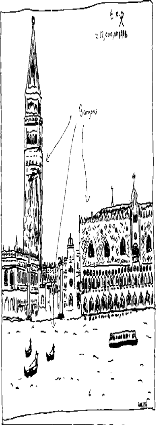
Figure 2: The Universe Today

There are three aspects of the above picture which are worth examining in detail. First, note that there is significant structure, second that all of the objects are baryonic, and third that the drawing captures a universe which is at least 12 Gyr old. All of these factors provide significant challenges to our current understanding of cosmology, including neutrino cosmology, as I will now describe.

2 Challenges for an $\Omega=1$ Universe

2.1 The Age Crisis

As long as the Universe is decelerating (i.e. if its energy density is dominated by matter or radiation) a strict upper bound on its age is given by:

$$t<{1\over{H_{0}}}$$ (1)

where $H_{0}=100hkms^{-1}Mpc^{-1}$. This result is straightforward to understand. If the Universe were expanding at a constant rate, then galaxies at a distance d from us will have taken a time $t=d/v={1\over{H_{0}}}$ to get to their current locations (where the second relation is obtained using Hubble’s Law, $v=H_{0}d$). If it is decelerating, then the time it took distant galaxies to reach their present positions must be less than this time. This provides a strict upper limit: $t<12.2Gyr[.8/h]$.

Of course, Einstein’s equations allow us to solve exactly for the age in many cosmological models. For a flat matter dominated universe:

$$t={2\over 3H_{0}}=8.14Gyr[.8/h]$$ (2)

Similarly, as long as $\Omega_{matter}>0.2$, even for an open, matter dominated universe we have

$$t<10.4Gyr[.8/h]$$ (3)

The big question, therefore, is: WHAT IS $h$ ?. With great certainty, we know today that $0<h<1$. With somewhat less certainty, recent observations have begun to narrow the range considerably. The initial HST measurement was [1] : $h=.8\pm.17$, while recent SN Ia light curve measurements tend to yield [2, 3] : $h=.55-.67$. A best estimate at the present time might therefore be $h=.7\pm.1$ (recognizing that all best estimates performed at earlier times have been different, and probably wrong, and that this estimate may suffer the same fate..). In this case, the above relations imply

$t<13.5Gyr$ (open universe (= ugly))

$t<10.5Gyr$ (flat universe (= beautiful))

The key question then becomes, Can the Universe be this Young? To answer this, we must resort to Cosmic Dating (not to be confused with something which is done in California singles bars…). This technique is based on the following theorem, which I will not prove here:

Theorem:    The age of the universe is greater than the age of the galaxy

We thus merely have to determine the age of the oldest objects in our galaxy. Among the oldest such objects are Globular Clusters, compact groups of up to thousands of stars located throughout the galaxy. By selecting out those clusters which have a large halo velocity, and heavy metal abundance less than $0.01\%$ of that of the sun, one is presumably sampling the among the oldest objects in the galaxy.

To determine the age of these objects is relatively simple, at least in principle. Star burn their hydrogen fuel at a rate which goes roughly as the third power of their mass. The time it takes therefore to burn the fuel is proportional to the total amount of fuel ($\approx M$) divided by the rate, or $M/M^{3}\approx M^{-2}$. Since this is a sensitive function of mass, if one can determine which mass stars are just exhausting their fuel now in any sample population of a fixed age, one can date the system.

Fortunately, there is a way to determine this mass. When plotted on a color-magnitude, or HR diagram, globular cluster stars lie in distinct patterns, corresponding to the “main sequence” stars, still burning hydrogen fuel, and stars which have turned off the main sequence and are now burning helium. Stars of higher mass start out higher on the main sequence, and therefore as time goes on, the “turnoff” point moves down the main sequence. By fitting the observed HR diagrams with theoretical isochrones, globular cluster ages can be determined. Traditionally best fits ages of 15-18 Gyr have resulted from such analyses. If this is true, then there is a big age problem, even for an open universe, if the hubble constant is larger than 55.

Since the Hubble age estimate is unambiguous for a fixed Hubble constant the crucial uncertainty in this comparison of globular cluster and Hubble ages resides in the globular cluster (GC) ages estimates. Rough arguments have been made that changes in various input parameters in the stellar evolution codes designed to derive globular cluster isochrones, or in the RR Lyrae distance estimator used to determine absolute magnitudes for GC stars, might change age estimates by 10-20 $\%$. However, no systematic study had been undertaken until recently to realistically estimate the cumulative effect of all existing observational and theoretical uncertainties in the GC age analysis. This was the purpose of a year long project in which I and my collaborators, Brian Chaboyer at CITA, Pierre Demarque at Yale, and Peter Kernan and CWRU became involved.

One of the such an analysis had not previously been carried out is that it is numerically intensive. Each run of a stellar evolution code for a single mass point takes 3-5 minutes on the fastest commercially available workstations. Nine different mass points at three different metallicity values must be run to produce each set of isochrones. If one then runs, say, 1000 different isochrone sets to explore the different parameter ranges available, this requires over 8 weeks of continuous processing time.

Because of the importance of this issue, we developed the necessary Monte Carlo algorithms. This involved first examining the measurements of input parameters in the stellar evolution code to determine their best fit values, and also their uncertainties along with the appropriate distributions to use in the Monte Carlo. Then the stellar evolution code and isochrone generation code were rewritten to allow sequential input of parameters chosen from these distributions, and output of the necessary color-magnitude (CM) diagram observables. Finally, we derived a fitting program to compare the predictions to the data. Since the numerically intensive part of this procedure involves the Monte Carlo generation of isochrones, by incorporating the chief observational CM uncertainty afterwards our results can quickly be refined as this uncertainty is refined.

We focussed on what we believe are the chief input uncertainties in the derivation of stellar evolution isochrones. These include: pp and CNO chain nuclear reaction rates, stellar opacity uncertainties, uncertainties in the treatment of convection and diffusion, helium abundance uncertainties, and uncertainties in the abundance of the $\alpha$-capture elements (O, Mg, Si, S, and Ca). Our stellar evolution code was revised to allow batch running with sequential input of these parameters chosen from underlying probability distributions. We did not include the equation of state among our Monte Carlo variables as it is now well understood in metal-poor main sequence stars.

A detailed discussion of the parameter choices and methodology can be found in our published work [4]. The bottom line is our result, given by the figure shown below.

Figure 3: The Distribution of Age Estimates for the Oldest Globular Clusters

Our results indicate that at the one sided 95$\%$ confidence level (determined by requiring 95$\%$ of the determined ages to fall above this value) a lower limit of approximately 12.1 Gyr can be placed on the mean value of these 18 Globular clusters. (The symmetric 95$\%$ range of ages about the mean value of 14.56 Gyr is 11.6-18.1 Gyr.) Note that the distribution deviates somewhat from Gaussian, as one might expect. In particular, at the lower age limits the rise is steeper than Gaussian, reflecting the fact that essentially all models give an age in excess of 10 Gyr, while the tail for larger ages is larger than gaussian. The explicit effect of the largest single common observational uncertainty, that in the RR Lyrae distance estimator, increases the net width of the distribution by approximately $\pm 0.6$ Gyr (i.e. $\approx\pm 5\%$). Note that simply varying this over its full $2\sigma$ range, keeping all other parameters fixed, would produce a $\pm 16\%$ change in GC ages estimates.

We believe that this result can now be used with some confidence to compare to cosmological age estimates. Of course, in addition to the age determined here one must add some estimate for the time it took our galactic stellar halo to form from the initial density perturbations present during the Big Bang expansion. Estimates for this formation time vary from 0.1 – 2 Gyr. To be conservative, one can choose the lower value. In this case, one finds that the age of globular clusters in our galaxy is inconsistent with a flat, matter dominated universe unless $h<0.54$, and for a nearly empty, matter dominated universe unless $h<0.80$. If the value of h is definitely determined to be larger than either of these values, some modification would seem to be required.

The most obvious modification, especially if one wants to preserve the beauty of a flat universe, is the addition of a small, non-zero cosmological constant (i.e. [5]). In this case, the relation between Hubble constant and age of the Universe is changed. For $\Omega_{\Lambda}+\Omega_{matter}=1$, one finds, for example

$$t=(2/3)ln([1+\Omega_{\Lambda}^{1/2}]/\Omega_{matter}^{1/2})H_{0}^{-1}\Omega_{\Lambda}^{-1/2}$$ (4)

This tends to infinity as $\Omega_{\Lambda}$ tends to unity. Since, as I shall argue later, a great deal of evidence suggests $\Omega_{\Lambda}<0.8$, this in turn implies

$$t\leq 1.08H_{0}^{-1}=13.2Gyr(.8/h)$$ (5)

In general, we can quantify the impact of the age problem by considering the space of $H_{0}$ vs $\Omega_{matter}$ for a flat universe with a cosmological constant. If the age of the universe, based on the Globular cluster age estimates, is $12<t<18$ Gyr, only the shaded region of phase space is allowed (the dashed line represents the lower bound on $H_{0}$ coming from the quote HST value with quoted error bar:

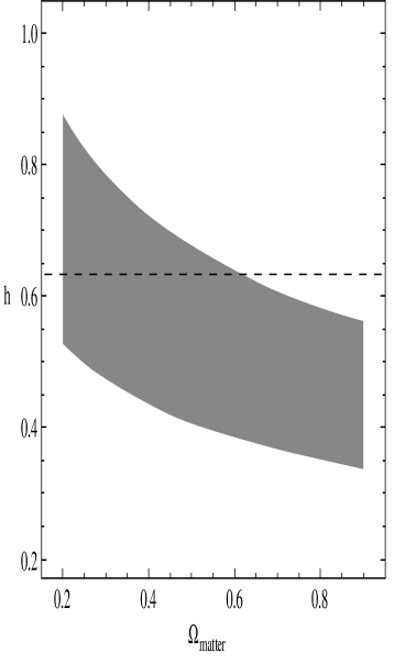
Figure 4: The Constraint on $H_{0}$ and $\Omega_{matter}$ for a flat universe, coming from the age of globular clusters

2.2 The Baryon Crisis

There has been a lot of discussion in the literature recently having to do with Crises in Cosmology… A particularly well publicized crisis of late is claimed to involve Big Bang Nucleosynthesis (BBN). Now the major crisis here may be that some people are claiming there is a crisis. However, in fact, BBN, makes a well defined prediction for the upper limit on the baryon density today which is not at all endangered by any new discussion of BBN uncertainties. This prediction be compared with other estimates of the baryon fraction of the Universe. It is here that there may indeed be a crisis for a flat universe, as I shall now briefly describe.

The main virtue of BBN has not changed over the past twenty five years. Because the predicted abundance today of each light element produced in the first seconds of the Big Bang explosion is a function of the abundance of protons and neutrons in the universe, a comparison of all of the cosmological light element abundance predictions with inferences based on observations today can yield constraints on $\Omega_{Baryon}$. If the allowed range is non-zero, we call this a success of BBN. If, on the other hand, the allowed range is zero, we call this a crisis.

An example of the predicted range, compared to possible limits based on inferences of “observed” light element abundances today is shown in the figure [6]

Figure 5: Light element abundance predictions from BBN

Several points should be noted. First, the predictions involve a band. This is because the predicted abundances are based on model calculations which are themselves based on measured nuclear reaction rates, which have uncertainties. Second, notice that the region of allowed $Y_{p}$, which corresponds to the mass fraction of He, if less than the dotted line, restricts the quantity $\eta$, which is directly related to $\Omega_{Baryon}$ to be less than some number, while the requirement that $D+^{3}He$ is less than the dotted line restricts $\eta$ to be greater than some number. Note also that these numbers are very close… leading to the possibility of a “crisis”.

The reason there is no crisis is simply that at this point the actual constraints coming from observations of light element abundances have huge systematic uncertainties associated with them. (i.e. [6, 7, 8]). So, one cannot say with any confidence that the range of allowed $\eta$ is vanishingly small.

Given this, one might suspect that perhaps all constraints on $\eta$ coming from BBN are suspect. This is incorrect. A firm upper bound on the baryon abundance today can still be placed, because the upper limits coming from utilizing ${}^{4}He$, $D+^{3}He$, and ${}^{6}Li$ EVEN INCORPORATING maximum possible systematic uncertainties all come together at the same value of $\eta$. To obviate this upper bound would require that all light element abundance measurements are wrong, which is far more unlikely than the assumption that some of them are wrong….. The firm upper limit from BBN can thus be quoted as [6, 7]

$$\Omega_{Baryon}\leq 0.26h^{-2}$$ (6)

Now, at this point you may be asking: What’s this got to do with an $\Omega=1$ Universe and massive neutrinos? The answer is that this constraint can be compared with a lower bound on the baryon abundance today which is obtained from measurements of X-Ray clusters of galaxies. These objects are among the largest structures known in the universe, and they are dominated by hot, X-Ray emitting gas. If one measures the temperature and luminosity of this gas as a function of position in the cluster, and if one assumes the gas is in hydrostatic equilibrium, and that it finds itself in a uniform, non-clumpy potential well, then one can derive directly the depth and shape of this potential well, and from that the total mass of the cluster. Also, one can derive a direct estimate of the mass of hot gas emitting the X-Ray luminosity. Thus, one can derive the ratio:

${M_{gas}\over M_{total}}={M_{baryon}\over M_{total}}$.

Now, IF these clusters probe the dominant mass density of the universe, then the above ratio is precisely equal to $\Omega_{Baryon}$.

What makes this particularly interesting is that a number of different groups have all recently derived this value for various rich clusters, and find that it is rather large. (i.e. [9, 10]). Allowing for the quoted range, and normalizing in the same way as I did for the BBN upper limit above, one finds the X-Ray Cluster constraint can be expressed:

$$\Omega_{Baryon}\geq 0.5-.08h^{-3/2}$$ (7)

Comparing this constraint with the one above, one sees a potential crisis unless either $h$ is very small, or, if X-Ray clusters are not probing all of the mass in the universe, (or, heaven forbid, the universe is open, and not flat—a possibility I shall not consider here in more detail because I find it so ugly). Indeed, if a significant fraction of the mass in the universe is unclustered, then the X-Ray bound would only correspond to the ratio $\Omega_{Baryon}/\Omega_{clusteredmatter}$. There are two possible physical situations which would correspond to this:

(1) The Cosmological Constant is Non-Zero, and the Universe is Flat: In this case, one derives a constraint on the $h$ vs $\Omega_{matter}$ space which is complementary to the earlier bound, and is shown in the figure along with the earlier bound.

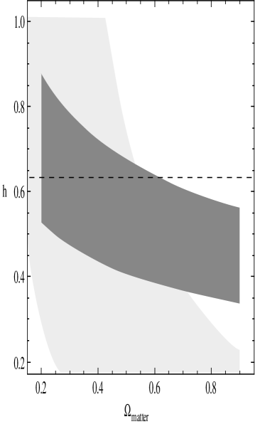
Figure 6: The Constraint on $H_{0}$ and $\Omega_{matter}$ for a flat universe, coming from the age of globular clusters and from baryon constraints

(2) There is unclustered matter (i.e. neutrinos!!!): Finally, for the first time in this lecture, I have referred to neutrinos directly. Light neutrinos, because they are “hot”, i.e. relativistic, until relatively late times, are not efficiently captured in clusters. Depending upon the mass of the neutrinos, and the fact that current mixed dark matter models (see following discussion) suggest a small admixture of light neutrinos along with cold dark matter in a flat universe, several authors have argued that this might alleviate the baryon crisis [11, 12]. However, both groups have found that quantitatively, things are only marginally improved. By allowing most of the light neutrinos to escape from galaxies, one finds that the X-Ray estimates for $\Omega_{Baryon}$ might overestimate the actual value by up to $25\%$. For acceptably small values of $h\approx 0.5$, this could resolve the crisis.

3 Challenges for a Flat Universe Involving Massive Neutrinos: Large Scale Structure

Now that I have finally introduced cosmological neutrinos as dark matter, I can introduce the third major crisis in modern cosmology which has revised the accepted orthodoxy regarding the prejudice of theorists of the nature of dark matter. This crisis has to do with Large Scale Structure. Put succinctly, the historical evolution of the theoretical Best fit model of the universe has been as follows:

1981:         $\Omega=1;\Omega_{\nu}=1;h\approx 0.5$

1985:         $\Omega=1;\Omega_{CDM}=1;h\approx 0.5$

1995:         $\Omega=?;\Omega_{CDM}<1;h>0.5$

As can be seen, current wisdom now allows, indeed perhaps requires, something other than Cold Dark Matter and Baryons in the Universe. Whether this something extra is neutrinos, or a cosmological constant, will perhaps be determined by further measurements of large scale structure.

Now the subject of Large Scale Structure and primordial density perturbations is far too complex to treat with any justice here. However, there is one aspect which gives an important constraint and which is relatively model independent while also being easily explained.

If one is going to posit, a priori, a spectrum of primordial density fluctuations, then the fourier space estimate would be of the following form:

$$({{\delta\rho}\over\rho})^{2}\approx k^{n}$$ (8)

The reason for this is simple. Anything but a power law would pick out some preferred scale at early times, and it seems unreasonable to expect that a scale of cosmologically interesting size would be fixed by the microphysics near t=0. Now, even before Inflationary model predictions, it was suggested that $n\approx 1$. This is because if n deviated significantly from unity, one would predict either too many primordial small black holes, or too large an anisotropy on large scales today.

Now, the above picture is that of the spectrum of primordial density fluctuations. However, the spectrum of fluctuations which eventually leads to galaxy formation is not the primordial one, but one which has rather been evolved by causal physics. Causality provides an important bit of structure. In particular, as long as there is any radiation in the universe today, the energy density of the Universe was once, at earlier times, dominated by this radiation. Thus, if the universe is matter dominated today, for all times earlier than some time $t_{eq}$ it was radiation dominated. Associated with this time will be some fourier mode $k_{eq}$, the wavelength of which is equal to the size of the horizon at this time. All modes with larger wavenumber will have a wavelength smaller than the horizon size, and can thus have been affected by earlier causal microphysical processes. It turns out that during a radiation dominated expansion, density fluctuations do not grow, and in fact can often be damped.

The net result of this causal behavior is that an initial spectrum which grows monitonically with $k$, can instead be transformed into a spectrum which is reduced somewhat starting around $k_{eq}$—hence there is some curvature to the evolved spectrum of density fluctuations for wavelengths corresponding to the region of $k_{eq}$. By measuring the two point correlation function of galaxies, one can hope to explore the evolved spectrum in this region, and compare it to predictions. The precise value of $k_{eq}$ will depend upon the time of matter-radiation equality, and hence upon the matter density today. Specifically, since $\rho_{matter}\approx\Omega_{matter}h^{2}$, and the relation between fourier modes and physical wavelengths scales as $1/h$, one finds that the value of $k_{eq}$ depends upon the combination $\Omega h$. Many different measurements of the shape of the spectrum of density fluctuations in the universe yield the constraint:

$$0.2<\Omega_{matter}h<0.3$$ (9)

This is perhaps the single most significant constraint coming from observations of Large Scale Structure which has altered our view of what might be the favored cosmological model in the past decade. Several options come to mind:

(1) $\Omega_{matter}<1$, and purely CDM. This implies either an ugly (open) universe, or a beautiful, flat universe, with a cosmological constant. Adding the constraint from the above equation to our earlier constaints then gives the following picture (where I have also introduced the constraint $\Omega_{matter}\geq 0.3$, as suggested by analyses of large scale peculiar velocity fields.) All of these constraints give a consistent picture[5] for $0.5<\Omega_{\Lambda}<0.7$.

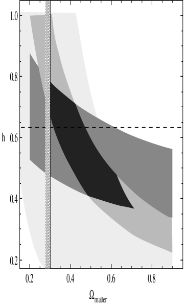
Figure 7: The Constraint on $H_{0}$ and $\Omega_{matter}$ for a flat universe, coming from the age of globular clusters, from baryon constraints, and from the power spectrum of density fluctuations at galaxy scales and larger, assuming an n=1 spectrum of primordial density fluctuations and no significant component of hot dark matter

(2) Change the shape of the primordial spectrum so that the shape near $k_{eq}$ shifts. This is possible if $n\neq 1$, for example.

OR,

(3) Change the value of $k_{eq}$ by changing the time of matter radiation equality: Both examples of such a behavior involve massive neutrinos. Prof. Sciama, who is was at this meeting, has proposed a scenario involving decaying neutrinos. Alternatively, by adding a hot component to the dark matter density, as one would get from light stable neutrinos, one will also change the epoch of matter radiation equality.

4 CHDM vs $\Lambda$CDM

If one is to preserve a flat universe today, it seems clear that one is being driven therefore by existing cosmological observations to one of two extremes. Either the Universe is dominated by a Cosmological Constant, or some fraction of the dark matter dominating the mass density of the universe today is in the form of light neutrinos. These two models present what have become the favored scenarios at the turn of the millenium. Whether either survives into the next millenium will depend upon how successfully various existing challenges are overcome.

(1) LSS Challenges for CHDM

(a) Early Galaxy formation

(b) The detailed Shape of the Power Spectrum

(c) the Void Probability function

(d) The Damped Lyman- $\alpha$ Forest.

All of these challenges come down to the same issue. Hot dark matter suppresses the growth of fluctuations on smaller scales. This will have the effect of causing galaxies to form later, reducing the magnitude of the power spectrum at small scales, changing the probabilities of large voids, and reducing the likelihood of producing significant clumped hydrogen clouds. Many authors have recently analyzed these issues, and at least two sets[13, 14] have suggested that these challenges can be successfully met, if the density of HDM is approx $\Omega_{\nu}\approx 0.2$, and if there are two species of light neutrinos both with a mass near 2 eV.

(2) LSS Challenges for $\Lambda$CDM

(a) Non-Linear Power on Small Scales

(b) The Deceleration Parameter

A cosmological constant dominated universe avoids the problem of the growth of small scale structure associated with mixed dark matter models. However, by avoiding this problem too efficiently, it might result in excessive structure on small scales. Recent numerical models have suggested, at least for the extreme value of $\Omega_{\Lambda}\approx 0.8$, that unacceptably large galaxy potential wells will form. Perhaps the biggest observational challenge which may arise in the near term for a cosmological constant dominated universe is the fact that such a universe will not be decelerating. As a result, if a careful measurement of the deceleration parameter becomes possible, as recent observations of SN 1a light curves suggest might be the case, one could rule out this scenario altogether. Indeed, very preliminary observations of Type 1a SN do suggest that the deceleration parameter is positive, which would require that the cosmological constant contribution to the energy density today not exceed that due to matter.

5 Conclusions

Which of these favored scenarios, if either, is more appealing? Well, beauty is in the eye of the beholder. To help guide the eye, however, I present my own scorecard, using the consumer’s digest convention, where an open circle is very bad, and a closed circle is very good. In this way, I compare CHDM,$\Lambda$CDM, and CDM flat models against constraints from age, the baryon abundance, the shape of the power spectrum of density fluctuations, small scale structure, and whether the model is theoretically contrived.

Figure 8: A Consumer’s Guide to Cosmological Models

I have no idea whether any of these models will survive the test of time, and observations. However, at the moment the choice seems clear: Neutrinos, or Nothing!

6 Acknowledgments

I would like to thank the organizers of the meeting for their kind hospitality and patience.

7 References

References

- [1] W. Freedman et al, Nature 371 (1994) 757.
- [2] D. Branch et al, astro-ph/9604006 preprint
- [3] A.G. Reiss et al, Ap. J. 438 (1995) L17
- [4] B. Chaboyer, P. Demarque, P. J. Kernan, L. M. Krauss, Science, 271 (1996) 957
- [5] L. M. Krauss and M. S. Turner, J. Gen. Rel. Grav. 27 (1995) 1137
- [6] L. M. Krauss and P.J. Kernan, Phys. Lett. B347, (1995) 347
- [7] C. Copi, D.N. Schramm, and M. Turner, Science 267 (1995) 192
- [8] M. Turner et al, Fermilab preprint 1996
- [9] S. D. M. White et al, Nature 366 (1993) 429
- [10] D. A. White and A. C. Fabian, M.N.R.A.S. 273 (1995) 73
- [11] L. Kofman et al ,UH-IfA -95/46 preprint
- [12] R. W. Strickland and D. N. Schramm, Fermilab pub 95/398-A
- [13] R. Somerville, J. R. Primack, R. Nolthenius, preprint, astro-ph/9604051
- [14] C-P Ma, Ap. J, to appear Nov 1996