ABSTRACT

I develop a method for assessing the ability of an instrument, coupled with an observing strategy, to measure the angular power spectrum of the cosmic microwave background (CMB). It allows for efficient calculation of expected parameter uncertainties. Related to this method is a means of graphically presenting, via the “eigenmode window function”, the sensitivity of an observation to different regions of the spectrum, which is a generalization of the traditional practice of presenting the trace of the window function. I apply these techniques to a balloon-borne bolometric instrument to be flown this spring (MSAM2). I find that a smoothly scanning secondary is better than a chopping one and that, in this case, a very simple analytic formula provides a good (40% or better) approximation to expected power spectrum uncertainties.

1 Introduction

Precision measurement of the angular power spectrum of the cosmic microwave background (CMB) promises enormous scientific returns. The expected results for the next generation of satellite experiments have been studied extensively [1, 2]. If one assumes that structure was formed by
gravitational instability then MAP [3] and COBRAS/SAMBA [4] should both measure $\Omega$, the Hubble constant and other cosmological parameters to better than a few per cent.

These large sky coverage, map-making observations lend themselves to easy analytic evaluation. However, there are very important balloon-borne and ground-based observations to be done over the next few years for which the determination of expected power spectrum uncertainties is not as straightforward. The method presented here is in principal analytic but the necessary high-dimensional linear algebra requires numerical work in practice.

One influence on the ability of any instrument to measure the microwave background is its ability to separate the CMB from confusing astrophysical foregrounds. Much work has been done along these lines [5, 6]. In contrast, relatively little attention has been paid to the choice of spatial observing strategy and its effect on expected power spectrum uncertainty. The benefits of high angular resolution have been emphasized [1] and it is well-known that a rough guide to optimal sky coverage in a fixed time is that which gives a signal-to-noise ratio per independent pixel of unity. However, the pixels are not independent, necessitating a more sophisticated analysis.

One reason for this discrepancy between attention paid to frequency
strategy versus spatial strategy is that while the spectrum of the CMB and confusing foregrounds have been known for a long time (at least roughly), it is only recently we have gained some knowledge of the angular power spectrum across a large range of angular scales. Prior to any detection of anisotropy, the only possible guidance on spatial strategy was that the optimal number of points to observe is thirteen [7]. Now that our knowledge has improved substantially, it should be used for the choice of observing strategies.

In section two I present the method and discuss the virtues of the eigenmode window function. In section three I derive a simple analytic approximation for power spectrum uncertainty. In section four I apply the method to the case of MSAM2 as an example. I use the example to make a quantitative argument for a smoothly scanning secondary as opposed to a chopping secondary, to present the eigenmode window function, and to compare the calculated power spectrum and cosmological parameter uncertainties with those from a simple analytic formula. An appendix details the calculation of the theory and noise covariance matrices and also suggests a useful prescription for normalizing window functions.

2 Semi-analytic Method

The data set can be modeled as consisting of signal and noise, $D_{i}=S_{i}+N_{i}$. Its covariance is:

$$\langle D_{i}D_{j}\rangle = \langle S_{i}S_{j}\rangle+\langle N_{i}N_{j}\rangle$$ (1)

$$= C^{S}_{ij}+C^{N}_{ij}$$ (2)

For the simple case where the $D_{i}$ are measurements of the temperature in directions enumerated by $i$, the signal covariance matrix is only a function of the angle separating $i$ and $j$, $\theta_{ij}$:

$$C^{S}_{ij}=C(\theta_{ij})=\sum_{l}{2l+1\over 4\pi}C_{l}P_{l}(\cos\theta_{ij})$$ (3)

where $C_{l}$ is called the angular power spectrum. For reasons to be discussed below, the data are generally not direct measurements of the temperature in a given direction, but are linear combinations of temperatures in several directions. Calculation of $C^{S}$ and $C^{N}$ in the general case is discussed in the appendix.

In general, the signal covariance matrix depends only on the observing strategy and the angular power spectrum $C_{l}$. We can think of the angular-power spectrum as a function of parameters, $a_{p}$, either physical ($\Omega_{0},n_{S},h,{\rm etc.}$) or phenomenological. The task at hand is to estimate, for a given experiment, the uncertainties to expect on the parameters $a_{p}$.

Our task is simplified by transforming the data so that both the signal and noise covariance matrices are diagonal. The desired transformation is the Karhunen-Loeve [8] transformation or, as it has become known in CMB phenomenology, the signal-to-noise eigenmode transformation [9]. Bond [10] and White and Bunn [11] used it in their analyses of the COBE DMR maps. Vogeley and Szalay have shown how it is useful for analysis of galaxy redshift surveys [12]. The transformation is a non-unitary mapping of the data in the pixel basis into the “signal-to-noise eigenmode” basis. The transformation to $D_{i}^{\prime}$ (the data in the S/N basis) is as follows:

$$D_{i}^{\prime}=R_{ij}((C^{N})^{-1/2})_{jk}D_{k}$$ (4)

where $C^{N}_{ij}\equiv\langle N_{i}N_{j}\rangle$, R is the rotation matrix that diagonalizes
$M\equiv(C^{N})^{-1/2}C^{S}(C^{N})^{-1/2}$ and $C^{S}_{ij}\equiv\langle S_{i}S_{j}\rangle$. It is straightforward to show that

$$\langle D_{i}^{\prime}D_{j}^{\prime}\rangle=(\lambda_{i}+1)\delta_{ij}$$ (5)

where $\lambda_{i}$ are the eigenvalues of the S/N matrix, $M$. Thus we have the desired transformation, since the signal and noise covariance matrices are now diagonal.

We can now think of the experiments as measuring the $\lambda_{i}$ which are a function of the power-spectrum and therefore of the parameters, $a_{p}$. We can build a quadratic estimator for $\lambda_{i}$ from $D_{i}^{\prime}$ by squaring it and subtracting unity:

$$\lambda_{i}^{\rm est}=D_{i}^{\prime 2}-1$$ (6)

This estimator has variance $2(\lambda_{i}+1)^{2}$ since $D_{i}^{\prime}$ is a Gaussian random variable with variance $\lambda_{i}+1$.

From here it is straightforward to calculate uncertainties on the parameters. First calculate the curvature matrix $\alpha$:

$$\alpha_{pp^{\prime}}=\sum_{i}{1\over\sigma^{2}(\lambda_{i})}{\partial\lambda_{i}\over\partial a_{p}}{\partial\lambda_{i}\over\partial a_{p^{\prime}}}.$$ (7)

where $\sigma^{2}(\lambda_{i})=2(\lambda_{i}+1)^{2}$. Then invert to get the desired result, the parameter covariance matrix [13, 2, 14]:

$$C^{P}_{pp^{\prime}}=\left(\alpha^{-1}\right)_{pp^{\prime}}.$$ (8)

Equation 8 is strictly true only if our estimates of $a_{p}$ are Gaussian random variables which will be the case if the eigenvalues depend linearly on $a_{p}$. In general the $\lambda_{i}$ have non-linear dependences on physical parameters, but if the data constrain the parameters sufficiently then the non-linear effects will be unimportant.

The covariance matrix is simply given by the inverse of the curvature matrix for the case when we have no prior information on the parameters. At the other extreme, if the parameters other than $a_{p}$ are perfectly known then $\sigma^{2}(a_{p})=1/\alpha_{pp}$. The intermediate case is easily treated if the prior information is expressed as a covariance matrix $C_{\rm prior}$. Then

$$\sigma^{2}(a_{p})=\left(\left(\alpha+C_{\rm prior}^{-1}\right)^{-1}\right)_{pp}.$$ (9)

To summarize, the procedure is straightforward. First choose a
parametrized theory and calculate the signal and noise covariance matrices. This step requires a specific choice of theory parameters. Calculate the rotation matrix, $R$, the eigenvalue spectrum, $\lambda_{i}$, and its derivatives. Calculate the curvature matrix, add any prior information and invert to get the estimated parameter covariance matrix.

The imaginary analysis of the data that I used above to derive Eq. 7 neglected off-diagonal terms that would be included in a full likelihood
analysis. A Taylor series expansion in the log of the likelihood function, about its maximum, leads to the result [15]

$$2\alpha_{pp^{\prime}}={\rm tr}[(C^{S}+C^{N})^{-1}{\partial C^{S}\over\partial a_{p}}(C^{S}+C^{N})^{-1}{\partial C^{S}\over\partial a_{p^{\prime}}}]$$ (10)

where tr stands for the trace. With a little algebra this becomes:

$$\alpha_{pp^{\prime}}=\sum_{i,j}{({\partial\lambda\over\partial a_{p}})_{ij}({\partial\lambda\over\partial a_{p^{\prime}}})_{ji}\over 2(\lambda_{i}+1)(\lambda_{j}+1)}.$$ (11)

The difference between the two results (Eq. 8 and Eq. 11) is simple to understand. The imaginary analysis above neglected the off-diagonal terms that arise when we move in parameter space, off of the parameters for which the signal matrix is diagonalized. In other words, although $\lambda$ is diagonal by design, its derivatives are not. Since the maximum likelihood is the “best” [16] estimator, the parameter variances following from Eq. 11 will be smaller than those from Eq. 8. I will refer to the use of Eq. 8 as the diagonal approximation and to Eq. 11 as “exact”, with quotations due to the implicit approximation of linear parameter dependence already mentioned.

Eq. 11 is an improvement on Eq. 10 because of the compression it allows; the modes below some level of signal-to-noise can be discarded. Because it neglects the off-diagonal terms, the diagonal approximation is even more convenient and in the applications that follow I show that the information loss from neglecting the off-diagonal terms is small.

Another advantage of the accuracy of the diagonal approximation is that it allows for easy visualization of how the observations will probe the spectrum. The window function $W_{lij}$ relates the power spectrum and its derivatives to the signal covariance matrix and its derivatives:

$${\partial C^{S}\over\partial a_{p}}=\sum_{l}{\partial C_{l}\over\partial a_{p}}{2l+1\over 4\pi}W_{l}$$ (12)

In the pixel basis the window function is complicated. The usual practice for indicating what region of the spectrum is probed is to plot only its trace – a procedure which neglects possibly important off-diagonal terms. It is possible to do much better in the eigenmode basis. From Eq. 12 follows:

$${\partial\lambda_{ij}\over\partial a_{p}}=\sum_{l}{\partial C_{l}\over\partial a_{p}}W_{lij}^{\prime}{2l+1\over 4\pi}$$ (13)

where the prime indicates the eigenmode basis. In this basis one can safely ignore the off-diagonal elements, reducing the number of relevant dimensions to two (one mulitpole moment index plus one pixel index), allowing for
visualization of all the important parts of the window function.

3 Simple Analytic Methods

For a map with uniform full-sky coverage and Gaussian angular resolution, $\sigma_{b}$, the eigenmodes are the spherical harmonics with eigenvalues equal to $wC_{l}e^{-l^{2}\sigma_{b}^{2}}$ where $w$ is the weight per solid angle. There are $2l+1$ modes for each $l$ and thus $\sigma^{2}(\lambda_{i})=2(\lambda_{i}+1)^{2}$ leads to the formula (derived by other means in [1]):

$$\sigma^{2}(C_{l})={2\over 2l+1}\left(C_{l}+w^{-1}e^{l^{2}\sigma_{b}^{2}}\right)^{2}.$$ (14)

The effect of observing only a fraction of the sky, $f$, can be approximately described by increasing the variance of $C_{l}$ by $f^{-1}$ since the number of modes is roughly proportional to the area [2, 17, 18]. Jungman et al. [2] used this formula and the analogs of Eq. 7 and 8 to calculate standard errors for an eleven parameter adiabatic gravitational instability model. The partial-sky corrected version of Eq. 14 must be used with care, however. The modes are no longer spherical harmonics and therefore any estimate for $C_{l}$ will be correlated with that of $C_{l}^{\prime}$ – a correlation with range $\Delta l\approx 2\pi/\theta$ where $\theta$ is a linear dimension of the observed field [19]. The equation only makes sense when the spectrum is binned with $\Delta l\mathrel{\mathchoice{\lower 3.6pt\vbox{\halign{$\mathsurround=0pt\displaystyle\hfil#\hfil$\cr>\crcr\sim\crcr}}}{\lower 3.6pt\vbox{\halign{$\mathsurround=0pt\textstyle\hfil#\hfil$\cr>\crcr\sim\crcr}}}{\lower 3.6pt\vbox{\halign{$\mathsurround=0pt\scriptstyle\hfil#\hfil$\cr>\crcr\sim\crcr}}}{\lower 3.6pt\vbox{\halign{$\mathsurround=0pt\scriptscriptstyle\hfil#\hfil$\cr>\crcr\sim\crcr}}}}2\pi/\theta$.

4 Application to MSAM2

In this section I apply the above formalism to the particular case of the second Medium Scale Anisotropy Measurement instrument (MSAM2). The MSAM instruments are balloon-borne off-axis Cassegraine telescopes with bolometric radiometers. The MSAM1 instrument is described in [20]. Detections have been reported from two of the flights [21] with the second flight confirming the results of the first [22]. The MSAM2 instrument uses the same gondola as MSAM1 but has a different radiometer and secondary mirror.

The largest component of atmospheric contamination depends only on elevation and is slowly varying in time. Thus a standard technique to reduce atmospheric contamination is to rapidly sample a stretch of sky at constant elevation by motion of a secondary mirror from $-\theta_{c}$ to $\theta_{c}$. Only linear combinations of the data that have no sensitivity to a spatially homogeneous signal are kept for further processing. In some cases those combinations sensitive to a gradient are discarded as well. Each linear combination corresponds to a “synthesized antenna pattern”. The MSAM1 secondary motion was a three point chop. From the time stream, two antenna patterns were synthesized.

The MSAM2 secondary motion will be a triangle wave pattern of period $T$. Here we model the time stream of data as follows:

$$d(t)=A_{0}(\theta_{i})/2+\sum_{\mu=1}^{8}D^{c}_{\mu}(\theta_{i})\cos(2\pi\mu{t\over T})+\sum_{\nu=1}^{8}D^{s}_{\nu}(\theta_{i})\sin(2\pi\nu{t\over T}).$$ (15)

where $\theta_{i}$ is a slowly changing function of time and refers to the point on the sky observed when the secondary is in its central position.

We cut the Fourier decomposition off at $\nu=\mu=8$ because the peak-to-peak chop amplitude is 8 beam full-widths; higher frequency modes would have very little signal. Since the secondary motion is symmetric about $t=T/2$, the asymmetric Fourier modes will contribute zero signal. Thus the odd $\nu$ components are ignored.

If we assume that the noise in the time stream $d(t)$ is white, then the noise in each of the above modes will be independent; the noise covariance matrix $C^{N}$ will be diagonal (see appendix). A better model would also have terms that vary in time but not in space, as is the case for instrumental and atmospheric drifts. Having to fit for the coefficients of these terms would induce correlations in the noise covariance matrix $C^{N}$. Given a model of the drifts it is possible to calculate $C^{N}$ but here I ignore these effects and take the matrix to be diagonal. From a model of the bolometer and the foregrounds [6] (a one component dust model) we expect the sensitivity to CMB to be NET $\simeq 266~{}\mu{\rm K}\sqrt{\rm sec}$.

Although the noise matrix is diagonal, the signal matrix is not. The off-diagonal correlations exist for three conceptually distinct reasons. First, the Fourier decomposition in Eq. 15 is for functions of period $T$ but because of the triangle wave motion of the secondary, the same stretch of sky is scanned twice in that one period. The $D_{\mu}^{c}(\theta_{i})$ and $D_{\mu}^{s}(\theta_{i})$ are the cosine and sine coefficients of the sky sampled from $\theta_{i}-\theta_{c}$ to $\theta_{i}+\theta_{c}$, with fundamental frequency half what it would be for a Fourier decomposition. Second, because the central position of the chopper changes over time, the decompositions do not all share the same origin. Thus, even if the fundamental mode had the right frequency, the modes with $\theta_{i}\neq\theta_{j}$ are not orthogonal. Third, since the sky is not “white” like the noise (there are intrinsic correlations) the different modes are correlated – even when $|\theta_{i}-\theta_{j}|>>2\theta_{c}$. The calculation of the signal covariance matrix, $C^{S}$, is described in the appendix.

4.1 Optimal Motion of the Secondary

Is it better to move the secondary in a step motion between two or three spots, or to smoothly scan it back and forth? Here I have addressed that question by computing the S/N eigenvalue spectra, shown in Figure 1, for a three-point chop and a triangle wave.

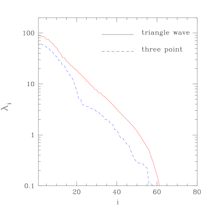
Figure 1: The S/N eigenvalue spectrum for a three-position secondary and for a smoothly scanning secondary.

The two curves shown in Fig. 1 are both S/N spectra for observing strategies that are the same in all respects except for the motion of their secondaries. They both point at a declination of $\delta=78$ degrees on the transit meridian as the secondary moves back and forth $\pm 80^{\prime}$ at constant declination (an approximation to the actual motion in cross-elevation). The beam is taken to be a Gaussian with $\sigma_{b}=20^{\prime}/(\sqrt{8ln2})$. The sky is observed in this manner for five hours. The rotation of the sky leads to coverage of a strip 15.6 degrees long. For a theory I took a flat spectrum with:

$$\delta T_{l}^{2}\equiv{l(l+1)C_{l}\over 2\pi}=(50~{}\mu{\rm K})^{2}.$$ (16)

The dashed curve is for the secondary that executes a three-point chop. The single difference and double difference signals are analyzed. The solid curve is for the triangle wave motion. In this case the signals from the 12 different synthesized antenna patterns were analyzed. One can see that the chopping secondary is inferior to the smoothly scanning ones since its eigenvalue spectrum is lower for every mode.

As a rough guide to the power-spectrum sensitivity of the experiment, we can simply count the number of modes with $\lambda_{i}>1$. This is because modes with $\lambda_{i}>>1$ all have the same fractional error ($\sqrt{2}$) while those with $\lambda_{i}<<1$ have very large uncertainties. For a more precise comparison we can perform the sum

$$\sigma^{2}(A)=\left(\sum_{i}{\lambda_{i}^{2}\over 2(\lambda_{i}+1)^{2}}\right)^{-1}$$ (17)

where $A$ is the amplitude of the spectrum whose shape has been assumed. For the triangle wave spectrum $\sigma(A)=0.22$.

It is easy to see how sensitivity to the amplitude of the spectrum will change with varying sky coverage. Increasing the sky coverage by a factor of $n$ will increase the number of modes by a factor of $n$. If the observing time remains fixed, then the noise in each pixel will increase, reducing each eigenvalue by a factor of $n$. From Fig. 1, we see that it would be highly beneficial to greatly increase the sky coverage.

The uncertainty in the amplitude has a very shallow minimum at $n=51$ of $\sigma(A)=0.087$. With such large sky coverage, the noise in each beam-size pixel is $97~{}\mu{\rm K}$. This is much larger than the signal in any of the synthesized antenna patterns but is just slightly smaller than the “stare mode” (undifferenced) signal of $120~{}\mu{\rm K}$. Thus we see that if one is solely interested in measuring an amplitude, setting the undifferenced signal-to-noise ratio to unity gives a near optimal sky coverage. However, the need to understand the inevitable non-idealities of the data argues against spreading the weight this thinly.

4.2 Band Estimates

The eigenvalue spectrum shows the sensitivity of the experiment to the overall amplitude of the spectrum but gives no indication of sensitivity to shape. To understand what regions of the spectrum are being probed it is useful to look at the eigenmode window function, shown in Fig. 2 for the triangle wave observations of the previous subsection. As expected, the peaks move to higher values of $l$ as the mode number increases.

Figure 2: A few modes of the eigenmode window function

Traditionally the region probed by an experiment has been indicated by the diagonal elements of the pixel basis window function, $W_{lii}$ [23]. This is adequate if all that is important is the $rms$ of the data. However, off-diagonal correlations are important as well and can significantly alter what regions of the spectrum are probed [24]. In particular it should be noted that as signal-to-noise ratio increases more information starts coming from the smaller scales – an effect that should be clear from Fig. 2. To quantify how well the experiment is probing different parts of the spectrum it is useful to estimate the uncertainty in several bands. To simplify interpretation it is useful to choose the bands with widths greater than the eigenmode window function widths since that will reduce the correlations between estimates. For Fig. 3 we have parametrized the spectrum as

$$\delta T_{l}=\cases{D_{1}&if $20\leq l<210$\cr D_{2}&if $210\leq l<400$\cr D_{3}&if $400\leq l<810$\cr}$$ (18)

and taken $D_{1}=D_{2}=D_{3}=50~{}\mu{\rm K}$. Note that estimating the power in a given band is very different from estimating the “band-power” for a synthesized antenna pattern. In the former we are using all the data to constrain part of the spectrum. In the latter we are using part of the data to constrain the entire spectrum.

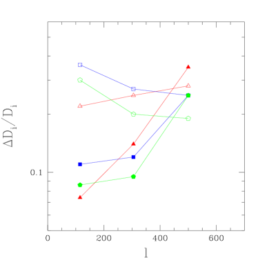
Figure 3: The expected fractional standard error for the three bands for the “parallel” (triangles) and “perpendicular” (squares) observing strategies (see text). The pentagons are the corresponding results from the analytic approximation. Filled symbols are for sixteen times as much area as for the open symbols; observing time is fixed at 5 hours.

The open triangles in Fig. 3 show the expected uncertainties for the triangle wave observing strategy described in the previous subsection. I will refer to this strategy as “parallel” since the sky coverage is swept out parallel to the motion of the secondary. The open squares are for a strategy where the sky is swept out perpendicular to the secondary motion. Each case has the same area: 5.2 sq. degrees, the same sensitivity, observing time, beam size, and even the same synthesized antenna patterns. The one long dimension of the “parallel” strategy is the reason for its superiority in the lowest spatial frequency bin.

The band estimates allow us to see the effect of varying sky coverage in more detail. The closed symbols in Fig. 3 are the expected uncertainties for observing 16 patches of the sky in the same way, with the same total observing time. The 16 patches are assumed to be far enough apart that the correlations between them can be ignored. In this case, the calculation is a simple extension of that done for the open symbols: the number of modes is increased by 16 and the S/N eigenvalues are all reduced by a factor of 16. Note that as expected, the lower the spatial frequency of the band, the more it benefits from extra sky coverage.

The “parallel” and “perpendicular” strategies are two extremely different ways of uniformly covering 5.2 sq. degrees. Despite this fact, the analytic approximation (pentagons), which does not depend on how the sky is covered, is good for both of them to better than 40%. Where the strategies are most different ($D_{1}$), it splits the difference! The results from the diagonal approximation (not shown) differ by at most 10%.

4.3 Cosmological Parameters

The sky coverage planned for the MSAM2 flight is too small to allow for simultaneous determination of a large number of cosmological parameters. However, it is interesting to vary a limited set of parameters and contrast the results from the “exact” formula with the diagonal approximation and the analytic approximation. To calculate the standard errors in the Table I varied the quadrupole, $\langle Q\rangle$, the scalar power-law index $n_{S}$ and $\Omega_{\rm tot}=\Omega_{0}+\Omega_{\Lambda}$ around their standard CDM values of $\langle Q\rangle=20~{}\mu{\rm K}$, $n_{S}=1$ and $\Omega_{\rm tot}=1$ [26]. For prior information, I assumed that COBE-DMR determined the quadrupole to within 20% [25]. Calculations were done for nominal and 16 times sky coverage.

Table 1: Constraints on Cosmological Parameters

Sky Coverage	Method	$\Delta\langle Q\rangle$	$\Delta n_{S}$	$\Delta\Omega_{\rm tot}$
1	Diagonal	4.0	0.27	0.35
1	“Exact”	4.0	0.22	0.28
1	Analytic	4.0	0.18	0.22
16	Diagonal	4.0	0.15	0.17
16	“Exact”	3.9	0.12	0.14
16	Analytic	3.9	0.11	0.12

It is not surprising that the diagonal approximation does worse here than for the band estimates since the diagonal is equal to the “exact” when the parameter is a normalizing constant. But even with these cosmological
parameters it is still good to 25%, bolstering the claim that the diagonal elements of the eigenmode window function hold most of the information. The analytic approximation, off by 20% at the worst, is even better here than for the band estimates. Note that the constraint on $\langle Q\rangle$ comes almost entirely from the prior information.

5 Discussion

The simple analytic approximation worked quite well for the cases studied. The approximation will be worse for observations where the differencing throws away more information, the off-diagonal noise is more important, or the sky coverage is less uniform. Differencing will throw away more information when the secondary throw to beam fwhm ratio is smaller or, as was explicitly shown, if the secondary chops discontinuously. On the other hand, we can expect the analytic formula to be a very good approximation for
partial sky map-making observations, such as those to come from Long Duration Ballooning.

Besides a method for estimating parameter uncertainties I have also
presented a useful tool for understanding how an observation probes the spectrum. Combined with a graph of the eigenvalue spectrum, the diagonal elements of the eigenmode window function allow one to immediately see the $\ell$-space resolution, the sensitivy to different regions of the spectrum, and the dependence of that sensitivity to varying sky coverage. The traditional use of the diagonal elements of the pixel basis window function can be misleading if the experiment has a high signal-to-noise ratio.

The bands in Fig. 3 were chosen with large widths to reduce correlations. However, these large widths mean some resolution has been discarded and thus this is not a good solution to the problem of presenting data in a compact, yet complete, manner. Further work along these lines is needed.

6 Acknowledgments

I would like to thank Andrew Jaffe, Max Tegmark, Martin White and my collaborators on MSAM2 for useful discussions as well as Grant Wilson, Shaul Hanany and Adrian Lee whose questions stimulated this work.

Appendix A Covariance Matrix Calculation

Given an observing strategy and a theory, we can construct the theoretical correlation matrix. Here I show how that calculation is done in general. For simplicity of notation, we assume that the telescope is pointed at $\theta_{i}$ for only one cycle of the secondary before moving on to $\theta_{j}$. In reality, many cycles are completed before the telescope’s pointing has changed significantly. Assume that the detectors are sampled $n$ times in one period $T$ and $\theta_{ia}$ is the direction on the sky observed on the $a^{\rm th}$ sample of the $i^{\rm th}$ secondary cycle. The multiple antenna patterns are synthesized by weighting the $n$ samples of each cycle by the weight vector $w_{\mu a}$:

$$D_{\mu i}={1\over n}\sum_{a=1}^{n}d_{ia}w_{\mu a}.$$ (19)

For example, the weight vectors for $D^{c}_{\mu}(\theta_{i})$ in Eq. 15 are

$$w_{\mu a}=\cos\left(2\pi\mu a/n\right)$$ (20)

To avoid proliferation of indices, we will now write, e.g., $D_{\mu i}$ as $D_{i}$ where $i$ is now understood to run over just pixels, just antenna patterns, or both, according to context. The data is once again modelled as due to signal from the microwave background, $S_{i}$ and noise from the atmosphere and instrument $N_{i}$. The time stream, $d_{ia}$ is also split into signal $s(\theta_{ia})$ and noise $n_{ia}$.

The two-point theoretical correlation function $C^{S}_{ij}\equiv\langle S_{i}S_{j}\rangle$ can be easily related to the intrinsic two-point correlation function $C^{s}(\theta_{ai},\theta_{bj})\equiv\langle s(\theta_{ai})s(\theta_{bj})\rangle$:

$$C^{S}_{ij}=\left({1\over n}\right)^{2}\sum_{a}\sum_{b}\langle s(\theta_{ia})s(\theta_{jb})\rangle w_{\mu a}w_{\nu b}.$$ (21)

By isotropy in the mean, $C^{s}(\theta_{ai},\theta_{bj})$ only depends on the angular distance, $\theta_{iajb}$, between $\theta^{i}_{a}$ and $\theta^{j}_{b}$. Thus, the correlation function can be decomposed into Legendre polynomials and Eq. 21 can be rewritten:

$$C^{S}_{ij}=\sum_{l}{2l+1\over 4\pi}C_{l}W_{lij}$$ (22)

where

$$W_{lij}\equiv\left({1\over n}\right)^{2}\sum_{a}\sum_{b}P_{l}\left(\cos(\theta_{iajb})\right)w_{ia}w_{jb}.$$ (23)

If the noise is white (uncorrelated from sample to sample) then the noise matrix

$$\langle\langle n_{i}n_{j}\rangle=n{{\rm NET}^{2}\over T}\delta_{ij}$$ (24)

and therefore

$$C^{N}_{ij}\equiv\langle N_{i}N_{j}\rangle={{\rm NET}^{2}\over T}\left({1\over n}\right)\sum_{k}w_{k}^{2}\delta_{ij}.$$ (25)

A convenient normalization prescription for the weight vector is to set $\sum_{i}w_{i}^{2}/n$ to a constant because then the variance in the noise is the same for every antenna pattern. Taking that constant to be unity, we find the variance in the noise for each antenna pattern is simply ${\rm NET}^{2}/t$ where $t$ is the total observing time – the same formula as for “stare mode”. This weight vector normalization is equivalent to a window function normalization and is actually a very sensible one. Since the NET is the same for all antenna patterns, the window functions with the higher signal-to-noise ratios will have larger amplitudes. Thus plotting the window functions normalized in this way allows for quick graphical comparson of both the l-space coverage and relative sensitivities of the various antenna patterns.

References

- [1] L. Knox, Phys. Rev. D 52, 4307 (1995).
- [2] G. Jungman, M. Kamionkowski, A. Kosowsky and D.N. Spergel, Phys. Rev. Lett. 76, 1007 (1996); Jungman et al., astro-ph/9512139.
- [3] E.L. Wright, G. Hinshaw and C.L. Bennett, Ap. J. 458, L53 (1996); http://map.gsfc.nasa.gov/.
-
[4]
M. Bersanelli,
et al., ESA Report
D/SCI(96)3;
http://astro.estec.esa.nl/SA-general/Projects/Cobras/cobras.html - [5] W.N. Brandt, C.R. Lawrence, A.C.S. Readhead, J.N. Pakianathan, and T.M. Fiola, Ap. J. 424, 1 (1994); M. Tegmark and G. Efstathiou, astro-ph/9507009, (1995).
- [6] S. Dodelson, astro-ph/9512021.
- [7] N. Kaiser, CITA, personal communication.
- [8] Karhunen, K. 1947, Uber lineare Methoden in der Wahrschleinlichkeitsrechnung, Helsinki: Kirjapaino oy. sana
- [9] J.R. Bond, Cosmic Structure Formation and the Background Radiation, in “Proc. IUCAA Dedication Ceremonies,” Pune, India, Dec. 1992, ed. T. Padmanabhan, Wiley (1994).
- [10] J.R. Bond, Phys. Rev. Lett. 74 4369 (1995).
- [11] M. White and E. Bunn, astro-ph 9503054.
- [12] M.S. Vogeley and A.S. Szalay, Ap. J., in press (1996).
- [13] W.H. Press, B. Flannery, S.A. Teukolsky and W.T. Vetterling, “Numerical Recipes in Fortran”, 2nd ed.
- [14] M. Tegmark, astro-ph/9511148, to appear in Proc. Enrico Fermi, Course CXXXII, Varenna, 1995.
- [15] M. Tegmark, A. N. Taylor and A. F. Heavens, astro-ph/9603021
- [16] The ML-estimator is asymptotically (in the limit of large data sets) the linear unbiased estimator with the smallest variance. See the review [15] and references therein.
- [17] M.P. Hobson and Joao Magueijo, astro-ph/9603064.
- [18] G. F. Smoot, astro-ph/9505139.
- [19] For an extensive discussion of spatial frequency resolution see M. Tegmark, Mon. Not. Roy. Astr. Soc. 280, 299 (1996), or [17].
- [20] D. J. Fixsen, et al., Ap. J. (1996), astro-ph/9512006.
- [21] E. S. Cheng, et al., Ap. J. 422, L37 (1994); E. S. Cheng, et al., Ap. J. 456, L71 (1996).
- [22] C. A. Inman, et al., astro-ph/9603017.
- [23] J.R. Bond, et al., Phys. Rev. Lett. 66, 2179 (1991).
- [24] The importance of off-diagonal correlations for the case of two-dimensional sky coverage by a chopping experiment was emphasized by M. Srednicki, M. White, D. Scott and E. Bunn, Phys. Rev. Lett. 71, 3747 (1993).
- [25] C. L. Bennett, et al., COBE Preprint 96-01, astro-ph/9606017
- [26] The angular power spectrum and its derivatives were kindly supplied by the authors of [2].