A Lagrangian Dynamical Theory for the Mass Function
of Cosmic Structures: II Statistics

Abstract

The statistical tools needed to obtain a mass function from realistic collapse time estimates are presented. Collapse dynamics has been dealt with in paper I of this series by means of the powerful Lagrangian perturbation theory and the simple ellipsoidal collapse model. The basic quantity considered here is the inverse collapse time $F$; it is a non-linear functional of the initial potential, with a non-Gaussian distribution. In the case of sharp $k$-space smoothing, it is demonstrated that the fraction of collapsed mass can be determined by extending to the $F$ process the diffusion formalism introduced by Bond et al. (1991). The problem is then reduced to a random walk with a moving absorbing barrier, and numerically solved; an accurate analytical fit, valid for small and moderate resolutions, is found. For Gaussian smoothing, the $F$ trajectories are strongly correlated in resolution. In this case, an approximation proposed by Peacock & Heavens (1990) can be used to determine the mass functions. Gaussian smoothing is preferred, as it optimizes the performances of dynamical predictions and stabilizes the $F$ trajectories. The relation between resolution and mass is treated at a heuristic level, and the consequences of this approximation are discussed. The resulting mass functions, compared to the classical Press & Schechter (1974) one, are shifted toward large masses (confirming the findings of Monaco 1995), and tend to give more intermediate-mass objects at the expense of small-mass objects. However, the small-mass part of the mass function, which depends on uncertain dynamics and is likely to be affected by uncertainties in the resolution–mass relation, is not considered a robust prediction of this theory.

1 Introduction

An important outcome of any cosmological model is the mass distribution of those cosmic collapsed structures which are predicted to form; this quantity is usually called mass function (hereafter MF) or multiplicity function. The theoretical determination of this quantity is difficult, as cosmological collapsed structures are the sites of non-linear gravitational dynamics. No exact analytical solution of the non-linear collapse of a general self-gravitating system is known. The first attempt to determine the number of collapsed objects was made by Press & Schechter (1974; hereafter PS); to predict the collapse of a mass clump, they used a heuristic argument based on the extrapolation of linear theory to the highly non-linear regime, and on the spherical collapse model, whose solutions are analytically known. Since PS, most works on the MF have been based on similar dynamical arguments.

However, a number of dynamical approximations have recently been developed. These approximations provide a reasonable description of the collapse of a self-gravitating, pressure-less fluid up to caustic formation, when the orbits of different mass elements cross each other (orbit crossing, hereafter OC, or shell crossing). In a previous paper (Monaco 1995, hereafter M95), the effects of non-spherical collapse were analyzed in a PS-like approach; in that case, the fraction of collapsed mass was identified with the probability of having suitable initial conditions such as to make a mass element collapse. The dynamical tools used in that case were the Zel’dovich approximation (Zel’dovich 1970) and the homogeneous ellipsoid collapse model.

This paper is the second in a series in which a new theory for the MF of cosmic structures is constructed. The idea, contained in M95, of constructing an MF based on realistic collapse dynamics, is the basis of the whole theory. The first paper of this series (Monaco 1996, hereafter paper I) develops the dynamical tools needed to obtain an MF. As already noted by M95, the MF dynamical problem (in its fluid limit) is intrinsically Lagrangian, in the sense that it is best faced within a Lagrangian fluidodynamical framework. Thus, all the tools of the Lagrangian formulation of gravitational dynamics can be used: the Zel’dovich approximation, Lagrangian perturbation theory (see, e.g, Bouchet et al. 1995; Buchert 1994; Catelan 1995; complete references are given in paper I), and the ellipsoidal collapse model. In paper I, all these dynamical approximations are analyzed, with the following results:

1. As in M95, the collapse of a mass element is identified with the OC instant; this definition has been amply discussed.

2. Lagrangian perturbations are applied to smoothed versions of the initial potential; it is assumed that smaller scales do not influence the collapse significantly.

3. The Lagrangian series, up to third order, converges in predicting the collapse of a homogeneous ellipsoid.

4. As a consequence, the collapse time of a homogeneous ellipsoid can be estimated in an easy and fast way by means of the third-order Lagrangian series, with a correction for quasi-spherical collapses.

5. Ellipsoidal collapse can be seen as a particular truncation of the Lagrangian series, when all the more than second derivatives of the initial peculiar gravitational potential are neglected.

6. In the general case of a Gaussian field with scale-free power spectrum, the Lagrangian series is shown to converge in predicting the collapse of a mass element, when fast-collapsing mass elements, representing at least 10 per cent of the mass, are taken into account. Convergence is valid at a qualitative level for about 50 per cent of the mass.

7. The homogeneous ellipsoidal collapse correctly reproduces the collapse time prediction of the Lagrangian series in the same convergence range.

The main quantitative outcome of paper I is the probability distribution function (hereafter PDF) of the inverse collapse times $F$ (in the spherical collapse case $F$ is just proportional to the density contrast). These are preferred to the collapse times as their distribution is better behaved: the inverse collapse times are large, but of order one, for fast collapsing points, and become smaller and smaller for slowly collapsing ones; non-collapsing points have vanishing or negative $F$ values.

This paper, paper II, faces the problem of finding an MF from the PDF of the inverse collapse times. The statistics needed to ‘count’ the objects, which form according to the dynamical predictions used in paper I, is developed, and the resulting MFs are analyzed and commented. A comparison of the whole theory to N-body simulations is underway (paper III). This paper is organized as follows: Section 2 contains an overview of the statistical procedures which have been developed by previous authors to obtain an MF; this is useful so as better to define the strategy for the statistical procedure to develop. In Section 3 the fraction of collapsed mass, as a function of the resolution, is determined for sharp $k$-space filtering. This quantity can be determined by solving a multi- (infinite-) dimensional diffusion process with an absorbing barrier; however, it is numerically shown that the same solution can be found by finding the first upcrossing rate of the $F$ process alone, as if $F$ were a Markov process; the precise behaviour of the $F$ process as a function of resolution is left as an open problem. Then, the determination of the MF can be reduced to a diffusion problem with a moving absorbing barrier. Numerical solutions and accurate analytical approximations for the fraction of collapsed mass are presented. In Section 4 the Gaussian smoothing case is analyzed. In this case the collapse time trajectories present strong correlations in resolution, which considerably complicate the problem. The results obtained from numerical simulations of individual trajectories are successfully compared to a reasonable approximation proposed by Peacock & Heavens (1990). The passage from the resolution variable to the mass variable is discussed in Section 5: a ‘missing piece’ is identified, related to the mass distribution of the extended collapsed structures. Section 6 contains a summary of the main results of the paper and some final comments.

2 Statistics and the MF: an Overview

Once a collapse condition is given for every point, and its statistical properties, namely its PDF, are known, a statistical framework has to be developed, to ‘count’ the number of collapsed structures. The main statistical procedures proposed in the literature are reviewed in the following. Throughout the paper the following notation will be used: the variable $\Lambda=\sigma_{\delta}^{2}$, equal to the mass variance, will be used as the resolution variable, $F$ will denote the inverse collapse time, and its PDF will be denoted as $P_{F}(F,\Lambda)$; in this Section, $F$ is generally equal to $\delta_{l}/\delta_{c}$, where $\delta_{l}$ is the linearly extrapolated density contrast and $\delta_{c}$ is a threshold. The growing mode $b(t)$ will be used as the physical time variable; it is demonstrated in paper I that this choice makes it possible to parameterize out the dependence of dynamics on the background cosmology with a great accuracy. The integral MF, i.e. the fraction of collapsed mass, will be denoted by $\Omega(<\Lambda)$ or $\Omega(>M)$, whether it is considered as a function of the resolution $\Lambda$ or of the mass $M$. Finally, the differential MF, the number of objects per unit volume and unit mass interval, will be denoted by $n(M)$, while $n(\Lambda)$ will denote the $\Lambda$ derivative of $\Omega(<\Lambda)$ (see Section 5 for the relation between the two $n$ functions).

In the seminal PS paper, a point was supposed to collapse whenever its linearly extrapolated density contrast, smoothed at a scale $R(\Lambda)$ with some filter, exceeded a given threshold $\delta_{c}$ (equal to 1.69 if the spherical collapse model was invoked). Thus, the fraction of collapsed mass at a given resolution was:

$$\Omega(<\Lambda)=\int_{F_{c}}^{\infty}P_{F}(F,\Lambda)dF\;;$$ (1)

($F_{c}$=1 if $F=\delta_{l}/\delta_{c}$). To get the MF as a function of the mass, $M$ was set equal to the mass contained by the smoothing filter; in the top-hat filter case, $M=4\pi\overline{\rho}R(\Lambda)^{3}/3$. When the filter is not a top-hat in real space, one can again obtain a relation between $\Lambda$ and $M$, even though its physical meaning is less clear (see, e.g., Bond et al. 1991).

One of the weaknesses of this statistical approach was immediately clear: for any threshold $\delta_{c}$ of order one, the integral in equation (1) tends to 1/2 as $\Lambda$ becomes very large, so that just one half of all the mass in the Universe is predicted to collapse; PS overcame this normalization problem by multiplying their MF by a ‘fudge’ factor of 2. This 1/2 factor is a signature of linear theory, which predicts that only initially overdense regions (one half of the total mass) are able to collapse. On the other hand, the lack of normalization of the PS MF is caused by the incorrect way of counting collapsed points. As a matter of fact, a collapse prediction is given to each point for any resolution $\Lambda$; in other words, a whole trajectory in the $F$–$\Lambda$ plane is assigned to each point. At small $\Lambda$ values (large $R$), all trajectories lie below the threshold, but when $\Lambda$ grows the trajectories can upcross or downcross the threshold. The first upcrossing is related to the collapse of the point at that scale; any further downcrossing is meaningless: a point which is collapsed at a scale $R$ (and is included in a region of size $\geq R$) cannot be considered as not collapsed at a smaller scale $R^{\prime}<R$ (and not included in any collapsed region of size $\geq R^{\prime}$). This fact was first recognized and solved by Epstein (1983), then by Peacock & Heavens (1990; hereafter PH) and by Bond et al. (1991; hereafter BCEK). To correct for this cloud-in-cloud problem, the integral MF has to be related to the probability $P_{F}^{\rm noup}(F,\Lambda)$ that a trajectory has never upcrossed the threshold:

$$\Omega(<\Lambda)=1-\int_{-\infty}^{F_{c}}P_{F}^{\rm noup}(F,\Lambda)dF\;.$$ (2)

The determination of $P_{F}^{\rm noup}(F,\Lambda)$ is generally difficult: $P_{F}^{\rm noup}(F,\Lambda)$ is the conditional probability of $F$ being $>F_{c}$ at $\Lambda$, given $F<F_{c}$ at all smaller $\Lambda$ values, so that all the N-point correlations of $F$ at different $\Lambda$ have to be considered. The problem is greatly simplified if the filter function is a top-hat in the Fourier space (sharp $k$-space filtering, hereafter SKS; see BCEK). In this case, provided the initial density field is a Gaussian process, independent modes are added as the resolution changes, and the trajectories in the $F$–$\Lambda$ plane are random walks ($F$ is a Markov process, in particular a Wiener process; see Section 3 for further details). Thus, the first upcrossing problem is equivalent to a random walk with a (fixed) absorbing barrier. The PDF of the trajectories obeys a Fokker-Planck equation (see equation 7):

$$\frac{\partial}{\partial\Lambda}P_{F}^{\rm noup}(F,\Lambda)=\frac{1}{2}\frac{\partial^{2}}{\partial F^{2}}P_{F}^{\rm noup}(F,\Lambda)\;,$$ (3)

with the boundary condition $P_{F}^{\rm noup}(F_{c},\Lambda)=0$. The solution is:

$$P_{F}^{\rm noup}(F,\Lambda)dF=$$

$$\frac{1}{\sqrt{2\pi\Lambda}}\left[\exp\left(-\frac{F^{2}}{2\Lambda}\right)-\exp\left(-\frac{(F-2F_{c})^{2}}{2\Lambda}\right)\right]dF\;.$$

With this solution, the resulting MF is the original PS one, including the ‘fudge’ factor 2:

$$n(\Lambda)d\Lambda=F_{c}\exp(-F_{c}^{2}/2\Lambda)/\sqrt{2\pi\Lambda^{3}}d\Lambda\;.$$ (5)

If the filter is not SKS, the $F$ trajectories are not random walks ($F$ is no longer a Markov process); they are affected by strong correlations, and no Fokker-Planck equation can be written for their PDF. In this case, the differential MF reduces to that of PS without the factor of 2 at large masses, and has a different slope at small masses; this was shown both by PH and by BCEK. Non-SKS filters are very difficult to deal with in this framework, as all the N-point correlation functions are relevant in determining the statistical properties of the trajectories. However, PH found a reasonable and successful way to approximate the $P_{F}^{\rm noup}(F,\Lambda)$ distribution; it will be described in Section 4.

The powerful and elegant diffusion formalism has been used to find the merging histories of dark-matter clumps, as the solutions of a two-barrier diffusion problem (BCEK; Lacey & Cole 1993); Bower (1991) obtained the same results as extensions of the original PS work, without using the diffusion formalism. Lacey & Cole (1994) made a number of empirical choices to optimize the adherence of their formulae to N-body simulations: they took the SKS solution, which coincides with the original PS solution, and is easier to deal with, and let two parameters vary, namely the threshold parameter $\delta_{c}$ and the mass assigned to the filter; with these choices, they succeeded in fitting the abundance and the merging histories of simulated friends-of-friends dark halos.

Another important problem of the PS statistical procedure was outlined by Blanchard, Valls-Gabaud & Mamon (1992) and Yano, Nagashima & Gouda (1996) (even though the same problem had already been faced in Epstein 1983). If the spherical top-hat model is used to predict the collapse time, and if top-hat smoothing is consistently used, then the density contrast in a point has to be interpreted as a mean over a spherical volume of radius $R$. As a consequence, a collapse prediction has to be considered as relative not simply to the point, but to the whole spherical region which surrounds it. The collapse condition has then to be changed to the following: a point collapses if it is embedded in a collapsing region, even though it is not at its center (and then its smoothed density contrast can be smaller than the threshold). In paper I this kind of reasoning has been called global interpretation of the collapse time. This new collapse condition considerably complicates the statistical problem; Blanchard et al. (1992) have shown this to cause a flattening of the MF with respect to the PS one, while Yano et al. (1996) have faced the problem by explicitly introducing the two-point correlation function in the collapse condition.

The PS procedure was extended in a number of other papers. In particular, Lucchin & Matarrese (1988) extended the PS formalism to non-Gaussian density fields and Lilje (1992) to general cosmologies. Porciani et al. (1996) tried to introduce non-Gaussianity in the diffusion framework by reflecting all the trajectories crossing $\delta_{l}=-1$, to avoid unphysical negative densities; in this way they found an intriguing cutoff of the MF at small masses. The same dynamical content as in the PS approach is present in the block model of Cole & Kaiser (1989) and in the Monte Carlo approach of Rodriguez & Thomas (1996).

In the PS framework, the relevant objects to be considered are the sets of points whose $F$ upcrosses a given threshold; these sets are usually called excursion sets. Alternatively, one can suppose that the forming structures are not connected to general excursion sets, but to the peaks of the initial density contrast (see, e.g., Bardeen et al. 1986). Then, counting structures is reduced to counting the number of peaks above a given threshold. With respect to the excursion set approach, the peak approach has a great advantage, namely that the extended structures which are to be counted are well defined, clearly connected to the peaks of the density field. However, the peak approach has a number of disadvantages: (i) going from excursion sets to peaks greatly complicates the formalism, as the peak constraint is much stronger than a simple threshold constraint; as a consequence, an analytical determination of the number of peaks is hopeless if $F$ is not a Gaussian or closely related process (except for high peaks; see Catelan, Lucchin & Matarrese 1988); (ii) obtaining an MF from the number of peaks requires an estimate of the mass associated to a peak. Different reasonable choices lead to different MFs (e.g., Ryden 1988; Colafrancesco, Lucchin & Matarrese 1989; PH; Cavaliere, Colafrancesco & Scaramella 1991); (iii) it is very difficult to solve the ‘peak-in-peak’ problem; this has been done by PH in a heuristic way, then by Appel & Jones (1990) and Manrique & Salvador-Sole (1995, 1996), and by Bond & Myers (1996) within their peak-patch theory; (iv) the peaks of the initial density field are generally not the first points to collapse; this has been shown by means of both theoretical arguments (see, e.g., Shandarin & Zel’dovich 1989: in the Zel’dovich approximations, structures are connected with the peaks of $\lambda_{1}$, the largest eigenvalue of the deformation tensor) and numerical simulations (Katz, Quinn & Gelb 1993; van de Weigaert & Babul 1994).

A different approach, pioneered by Silk & White (1978) and Lucchin (1989), was used by Cavaliere and coworkers; see Cavaliere, Menci & Tozzi (1994) for a recent review and paper I for further comments. In their case, the existence of an MF is implicit, and kinetic evolution equations are given for its evolution; this is at variance with the PS and related approaches, where the MF is obtained from the evolution of the density contrast field. Besides, in their application of the Cayley tree formalism to the adhesion approximation (Cavaliere, Menci & Tozzi 1996; see also Vergassola et al. 1995), the objects were identified with shocks in the collapsing medium.

To determine the MF from the statistics of the $F$ process, the excursion set approach has been chosen. It will be shown in the following that, in the SKS smoothing case, despite the complicate non-Gaussian nature of $F$, the MF problem can be recast in terms of a random walk with a moving absorbing barrier, while in the Gaussian filter case the useful approximation proposed by PH applies. A peak approach applied to the process $F$ would better take into account the complex geometry of the collapsed regions in the Lagrangian space, but, as mentioned before, it is intractable from the analytical point of view.

Some remarks about the $F$ process, already outlined in paper I, are worth stressing again:

1. As $F$ is (the inverse of) a time, any threshold $F_{c}$ in this theory simply specifies the time at which the MF is examined; there is no free $\delta_{c}$ parameter.

2. Smoothing is necessary because of the truncated nature of the dynamical approximations used. Thus the shape of the filter has to be chosen in order to optimize the performances of the dynamical predictions; usually Gaussian filters are preferred.

3. The dynamical predictions are strictly punctual; in other words, a point collapses only if it is predicted to collapse (at a given scale), not if a neighboring collapsing point is able to involve it in its collapse.

Point (i) is a result of the more detailed dynamics contained in this MF theory. Point (ii) implies that, even though we still have some freedom in choosing the shape of the filter, the Gaussian filter case has to be regarded as the most “physical” one. Point (iii) is connected to the discussion about the global interpretation of collapse times: in the Lagrangian perturbation case dynamical predictions are punctual, then the complications introduced by the global interpretation are avoided. Moreover, spherical symmetry of collapsed regions in Lagrangian space is not imposed, as it happened with the global interpretation of spherical collapse time. On the other hand, the exact size of the collapsed regions cannot be so easily determined as in the spherical case: as a consequence of the coherence of the underlying initial field, a point collapsed at a scale $R(\Lambda)$ will be part of a structure of typical size $R$ (or larger), but the exact determination of its size requires knowledge of the space correlations of the process $F$. In other words, the difficulties skipped in the diffusion problem, thanks to the punctual interpretation of the collapse time, are found again in the $\Lambda\rightarrow M$ transformation. This will be analyzed in Section 5.

Before going on, it is worth commenting on the physical meaning of the absorbing barrier in the Lagrangian dynamical context. The nature of the dynamical prediction is such that most mass is predicted to collapse at small scales (92 per cent according, for instance, to the Zel’dovich approximation); the exact number is not easy to determine, as the behavior of the strongest underdensities is not well predicted by Lagrangian perturbation theory (see paper I). Anyway, it is unlikely that about 10 per cent of mass in the strongest underdensities is going to affect the MF in any observable mass range. Thus, the diffusion formalism is not needed here just to ensure a correct normalization, which is more or less guaranteed, but to solve the cloud-in-cloud inconsistency of the original PS procedure, which in this context has the following meaning. As the power spectrum has no (or a very small) intrinsic truncation, a collapse prediction is assigned for every resolution to every point; these collapse predictions all have, in principle, the same validity. Recalling that collapse means to be enveloped in an OC region, it is natural to expect any point to be in OC at a small enough scale, and to be in single-stream regime at a large enough scale. The PS statistical procedure would suffice to find $n(\Lambda)$ if the transition to OC occurred only once, i.e. if the process $F$ never downcrossed the $F_{c}$ barrier. A downcrossing of $F$ has the following meaning: a point is in OC at a large scale, but it is not at a smaller scale; this appears contradictory, as a collapsed structure does not contain non-collapsed subclumps. To overcome this inconsistency, it is assumed that OC at one scale implies OC at all smaller scales. This corresponds to absorbing the trajectories of the $F$ process that upcross the $F_{c}$ barrier.

3 Sharp $k$-space Smoothing

The quantity $F(\Lambda)$ is a non-linear and non-local functional of the initial (peculiar rescaled) potential $\varphi({\bf q};\Lambda)$. Then, it is not trivial to infer the properties of the $F$ process as a function of $\Lambda$. In the following, it will be shown that the multi- (infinite-) dimensional process, defined by all the $F$ and $\varphi$ values in all the points, is a Markov process, so that the statistics of first upcrossing of $F$ can in principle be found by solving a multi- (infinite-) dimensional Fokker-Planck (hereafter FP) equation. It will also be shown that the same first upcrossing statistics can be reproduced by studying a (one dimensional) Markov process with the same PDF as the $F$ process.

It is opportune, before going on, to introduce a number of definitions which will be necessary in the following; a more detailed presentation can be found, for instance, in the textbooks by Arnold (1973) and Risken (1989).

Let $\xi(\Lambda)$ be a real stochastic process. Let’s denote by $x$ the value that the process $\xi$ takes at the resolution $\Lambda$. The process $\xi$ is said to possess the Markov property if its history at resolutions $>\Lambda$ is determined by its value $x$ at $\Lambda$, independently of its past history; in other words, a process possesses the Markov property if past and future are independent once the present is known.

A Markov process is called a diffusion process if its trajectories are continuous and if the quantities $D^{(1)}$ and $D^{(2)}$ exist:

$$\langle\xi(\Lambda+d\Lambda)-\xi(\Lambda)\rangle = D^{(1)}d\Lambda+{\cal O}(d\Lambda^{2})$$ (6)

$$\langle(\xi(\Lambda+d\Lambda)-\xi(\Lambda))^{2}\rangle = D^{(2)}d\Lambda+{\cal O}(d\Lambda^{2})\;.$$

The coefficients $D^{(1)}$ and $D^{(2)}$ are called drift and diffusion coefficients. The PDF $P_{x}(x,\Lambda)$ of a diffusion process obeys a FP equation:

$$\frac{\partial}{\partial\Lambda}P_{x}(x,\Lambda)=\left[-\frac{\partial}{\partial x}D^{(1)}(x,\Lambda)+\frac{1}{2}\frac{\partial^{2}}{\partial x^{2}}D^{(2)}(x,\Lambda)\right]P_{x}(x,\Lambda)\;.$$ (7)

A diffusion process with $D^{(1)}=0$ and $D^{(2)}=1$ is called a Wiener process, ${\rm W}(\Lambda)$. Its increments are uncorrelated: $\langle d{\rm W}(\Lambda)d{\rm W}(\Lambda^{\prime})\rangle=\delta_{D}(\Lambda-\Lambda^{\prime})$ ($\delta_{D}$ is the Dirac delta function), while $\langle{\rm W}(\Lambda){\rm W}(\Lambda^{\prime})\rangle=\min(\Lambda,\Lambda^{\prime})$. The transition probability from $\Lambda$ to $\Lambda^{\prime}$ is a Gaussian with variance $(\Lambda-\Lambda^{\prime})$, and the PDF at resolution $\Lambda$ is a Gaussian with variance $\Lambda$ and zero mean. All these definitions can be easily extended to the case of multi-dimensional processes.

In order to simplify the notation, in the following a stochastic process and its numerical values, although different mathematical objects, will be denoted by the same symbol.

3.1 A FP Equation for $P_{F}(F,\Lambda)$

It is useful to analyze first, as an example, the simple case of Zeldovich approximation in 2D. Initial conditions are given by the three independent component of the first-order deformation tensor (a symmetric 2D matrix), $w_{1}$, $w_{2}$ and $w_{3}$, the third one being the non-diagonal component. The two eigenvalues of the deformation tensor, $\lambda_{1}$ and $\lambda_{2}$, are simply:

$$\lambda_{1,2}=\frac{1}{2}\left(w_{1}+w_{2}\pm\sqrt{(w_{1}-w_{2})^{2}+4w_{3}^{2}}\right)\;,$$ (8)

where the $+$ sign corresponds to the largest eigenvalue $\lambda_{1}\equiv F$.

The three $w_{i}$ components, being linearly connected to the initial potential $\varphi$, are correlated Gaussian variables and, as functions of $\Lambda$, Wiener processes, with nonvanishing mutual correlations at fixed resolutions. Such processes constitute a 3D diffusion process; the evolution of their joint PDF is then controlled by a 3D FP equation with vanishing drift and constant diffusion ($D^{(2w)}_{ij}$) coefficients. Collapse is assumed to have place if:

$$F\equiv\lambda_{1}(w_{1}(\Lambda),w_{2}(\Lambda),w_{3}(\Lambda))>F_{c}\;.$$ (9)

Then, the first upcrossing rate problem can be formulated in term of a 3D diffusion with a complicate absorbing barrier.

On the other hand, the system $\{\lambda_{1},\lambda_{2},w_{3}\}$ can be obtained by means of a non-linear transformation of the $\{w_{i}\}$ system; it is easy to verify that such transformation is invertible and twice differentiable in any point, except in the line $w_{1}=w_{2}$ and $w_{3}=0$, a set of zero measure which is explicitly avoided by trajectories (as in the 3D case; see the joint PDF of eigenvalues, e.g., in M95). In this case, the $\{\lambda_{i}\}$ (with $\lambda_{3}\equiv w_{3}$) system is a Markov process, and, more precisely, a diffusion process (Arnold 1973; Risken 1989). The drift and diffusion coefficients can be found by means of the following transformation rules:

$$D^{(1)}_{i}=\frac{\partial^{2}\lambda_{i}}{\partial w_{j}\partial w_{k}}D^{(2w)}_{jk}$$ (10)

$$D^{(2)}_{ij}=\frac{\partial\lambda_{i}}{\partial w_{k}}\frac{\partial\lambda_{j}}{\partial w_{l}}D^{(2w)}_{kl}\;.$$

Then, the problem can be reformulated by means of a more complicate FP equation with the simple barrier $F=F_{c}$.

The same considerations can be generalized to any sufficiently well-behaved inverse collapse time $F$ in 3D. Let $\varphi({\bf q})$ be a Gaussian process in the Lagrangian space ${\bf q}$ (see paper I for the definition of Eulerian and Lagrangian coordinates). $\varphi$ is the initial peculiar rescaled gravitational potential, defined by the equation:

$$\nabla^{2}\varphi({\bf q})=\delta_{l}({\bf q})\;,$$ (11)

where $\delta_{l}({\bf q})=\delta_{0}({\bf q})/b_{0}$ is the linear density contrast ($\delta_{0}$ is the initial density contrast and $b_{0}\simeq a_{0}$ is the initial growing mode, nearly equal to the initial scale factor). This Gaussian process is assumed to have power at all relevant scales, up to a very small cutoff. From the field $\varphi$ a hierarchy of smoothed fields is obtained:

$$\varphi({\bf q})\rightarrow\varphi({\bf q};\Lambda)=\varphi({\bf q})*W({\bf q},\Lambda)\;,$$ (12)

where $*$ denotes a convolution, and $W({\bf q},\Lambda)$ is the SKS filter, which in the Fourier space is $\theta(1-kR(\Lambda))$.

The inverse collapse time $F({\bf q},\Lambda)$ of a point is a functional acting on the $\varphi$ potential:

$$F({\bf q},\Lambda)=b_{c}^{-1}({\bf q},\Lambda)={\cal F}_{\bf q}[\varphi({\bf q}^{\prime},\Lambda)]\;.$$ (13)

It is important to note that the functional ${\cal F}$ does not act directly on the $\Lambda$ variable; in other words, it does not shuffle information coming from different resolutions. In many cases it is not possible to obtain the explicit form of this functional (see paper I for full details). Anyway, it will always be assumed that it is twice differentiable with respect to the $\varphi$ values, except in some possible degenerate cases, which constitute a set of zero measure in Lagrangian space.

It is convenient, in order to handle the functional ${\cal F}$ introduced above, to consider discrete spaces; all the considerations which follow will be valid in the continuum limit. Let’s then consider the (Lagrangian) space divided into a large number $N$ of points $\{{\bf q}_{i}\}$:

$$F({\bf q},\Lambda) \rightarrow F({\bf q}_{i},\Lambda)=F_{i}(\Lambda)$$

$$\varphi({\bf q},\Lambda) \rightarrow \varphi({\bf q}_{i},\Lambda)=\varphi_{i}(\Lambda)$$ (14)

$${\cal F}_{\bf q}[\varphi({\bf q}^{\prime},\Lambda)] \rightarrow {\cal F}_{{\bf q}_{i}}(\{\varphi({\bf q}_{j},\Lambda)\})={\cal F}_{i}(\{\varphi_{j}(\Lambda)\})\;.$$

In this way the functional becomes an ordinary (non-linear) function of the $N$ resolution-dependent variables $\{\varphi_{i}(\Lambda)\}$.

The evolution equations of the $\{\varphi_{i}\}$ variables are those of a vector Wiener process. They can be written as follows:

$$d\varphi_{i}=f_{ij}(\Lambda)d{\rm W}_{j}$$ (15)

(summation over repeated indexes is meant), where $\{d{\rm W}_{j}\}$ are $N$ independent Wiener processes. The $f_{ij}(\Lambda)$ coefficients are such as to give the correct variances and spatial correlations of $\varphi$. Note the use of the differential notation in equation (15), which is common in stochastic mathematics, as time derivatives are ill-defined in this context.

It is possible to find evolution equations for the functions $F_{i}(\Lambda)$. With a chain-rule differentiation, assuming twice differentiability, the following system is obtained:

$$dF_{i} = \frac{\partial{\cal F}_{i}}{\partial\varphi_{j}}(\{\varphi\})d\varphi_{j}$$ (16)

$$d\varphi_{i} = f_{ij}(\Lambda)d{\rm W}_{j}\;.$$

This is a non-linear Langevin system. As mentioned above, this implies that the whole system $\{F,\varphi\}$ is a Markov process; provided the regularity conditions given above (eq. 6) are satisfied, the system is a diffusion process (see Arnold 1973 and Risken 1989 for a complete demonstration). Then, the evolution of $P_{\{F,\varphi\}}$, the joint PDF of the $F$ and $\varphi$ values in all the points, is given by a FP equation:

$$\frac{\partial P_{\{y_{i}\}}}{\partial\Lambda}=\left[-\frac{\partial}{\partial y_{i}}D^{(1)}_{i}(\{y_{i}\})+\frac{1}{2}\frac{\partial^{2}}{\partial y_{i}\partial y_{j}}D^{(2)}_{ij}(\{y_{i}\})\right]P_{\{y_{i}\}}\;,$$ (17)

where $y_{i}$ denote the components of the $\{F,\varphi\}$ vector. To find the first upcrossing rate, e.g., of the $F_{1}$ process (evaluated at ${\bf q}_{1}$) above the barrier $F_{c}$, such equation has to be solved with the constraint $P_{\{F,\varphi\}}(F_{1}=F_{c},\ldots)=0$.

Provided the $\{\varphi\}\rightarrow\{F\}$ transformation is a well defined and invertible one, the $\{F\}$ system is a Markov process by itself, and the problem can be formulated in terms of the $\{F\}$ system only.

A solution of such a multi-dimensional problem, while revealing the Markov nature of the problem, is not convenient in practice. A great simplification would come from reducing such a multi-dimensional problem to a one-dimensional one. As the 1-point PDF of the F process alone is known, it is possible to construct a FP equation whose solution is $P_{F}(F,\Lambda)$; if $F$ were a Markov process, the constrained solutions of the 1D FP equation would give the right solution for its first-upcrossing rate. However, there seems to be no simple reason to conclude that $F$ is a Markov process: the components of a multi-dimensional Markov process can possess not the Markov property (see, e.g., the example given in Risken 1989, Section 3.5); moreover, it is not possible to obtain a FP equation for $F=\lambda_{1}$ by integrating out all the other variables in the FP equation (17), as the drift and diffusion coefficients are not constant and then cannot be taken out of the integrals.

The solution of the 1D problem can anyway be considered as an ansätz to the true solution; it can be checked a posteriori, by means of direct numerical calculations, whether such ansätz leads to a correct description of the exact first upcrossing rate. This will be done in next Subsection, where it will be shown that the 1D solution leads to an almost perfect description of the first upcrossing rate problem. The numerical demonstration of this fact is sufficient for the scope of this paper, but leaves the question open of the reason of such behaviour, and of the possible Markov nature of the $F$ process. Such complex problems will be addressed in future work.

To construct a FP equation whose solution, with initial condition $P_{F}(F,0)=\delta_{D}(F)$ and natural boundary conditions ($P_{F}(F,\Lambda)$ and its $F$-derivative vanish at infinity), is $P_{F}(F,\Lambda)$(as given in paper I), it is convenient to transform the $P_{F}(F,\Lambda)$ distribution to a Gaussian distribution with variance $\Lambda$, $P_{x}(x,\Lambda)$. The $x(F)$ transformation for $\Lambda=1$ is given in paper I for the $F$ processes corresponding to ellipsoidal collapse (hereafter ELL) and third-order Lagrangian collapse (hereafter 3RD). To obtain the $P_{F}(F,\Lambda)$ distribution and the $x(F)$ transformation at any $\Lambda$, the following self-similarity property can be used: $P(F/\sqrt{\Lambda})dF/\sqrt{\Lambda}={\rm const}$; this is also valid for the $P_{x}(x,\Lambda)$ distribution. Then,

$$P_{F}(F,\Lambda)dF = \sqrt{\Lambda}\,P_{F}(F/\sqrt{\Lambda},1)dF$$ (18)

$$x(F,\Lambda) = \sqrt{\Lambda}\,x(F/\sqrt{\Lambda},1)\;.$$

With this transformations, the unconstrained PDF of the transformed quantity $x$ is virtually identical to the distribution of the linear density contrast $\delta_{l}$ (this is true at the 1-point level; the N-point PDFs of the transformed quantities $x$ at different points will generally not be Gaussian multivariates). The FP equation which admits $P_{x}(x,\Lambda)$ as a solution is obviously that of a Wiener process:

$$\frac{\partial}{\partial\Lambda}P_{x}(x,\Lambda)=\frac{1}{2}\frac{\partial^{2}}{\partial x^{2}}P_{x}(x,\Lambda)\;.$$ (19)

Transforming back to the $F$ variable, the FP equation for the $P_{F}(F,\Lambda)$ distribution is obtained; its drift and diffusion coefficients are:

$$D^{(1)}_{F} = -\left(\frac{\partial x}{\partial\Lambda}+\frac{1}{2}\frac{\partial^{2}x}{\partial F^{2}}\left(\frac{\partial x}{\partial F}\right)^{-2}\right)\left(\frac{\partial x}{\partial F}\right)^{-1}$$ (20)

$$D^{(2)}_{F} = \frac{1}{2}\left(\frac{\partial x}{\partial F}\right)^{-2}\;.$$

If the transformation is linear, $x=aF+b\sqrt{\Lambda}$, then the two coefficients become:

$$D^{(1)}_{F} = -\frac{b}{2a\sqrt{\Lambda}}$$

$$D^{(2)}_{F} = \frac{1}{2a^{2}}\;.$$ (21)

However, it is convenient to work directly with the $x$ process, whose FP equation is much simpler.

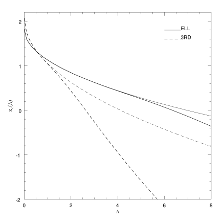
Figure 1: The $x_{c}(\Lambda)$ barriers for the ELL and 3RD predictions (heavy lines), together with their ‘linear’ part (light lines).

To find the distribution of the trajectories which have not upcrossed a given threshold $F_{c}$, the FP equation for $F$ has to be solved with the boundary condition $P_{F}(F_{c},\Lambda)=0$. Transforming this condition back to the $x$ variable, as the $F\rightarrow x$ transformation is time-dependent, the absorbing barrier for the $x$ process will move as $\Lambda$ grows. Then, the MF problem is reduced to a Wiener diffusion problem with a moving absorbing barrier.

3.2 The solution of the Moving Barrier Problem

The diffusion problem with a fixed absorbing barrier, equivalent to the solution of the FP equation (19) with boundary condition $P_{x}(x_{c},\Lambda)=0$, and with initial condition $P_{x}(x,0)=\delta_{D}(x)$, has a solution that has long been known (Chandrasekhar 1943), which can be obtained in the following way: the initial condition is changed to $P_{x}(x,0)=\delta_{D}(x)-\delta_{D}(2x_{c}-x)$, i.e. a negative image is put in a position symmetric with respect to the barrier. In the subsequent evolution, the boundary condition is satisfied at any time by symmetry. It is easy to see that the initial condition just shown leads to equation (2) as a solution (with $x$ instead of $F$). This solution formally turns negative beyond $x_{c}$; the true solution is obviously null there. Note also that no meaningful solution exists if $x_{c}<0$: all the trajectories are absorbed from the start.

Figure 2: ELL prediction, linear barrier, SKS smoothing. a) $P_{x}^{\rm noup}(x,\Lambda)$ and $P_{x}^{\rm fb}(x,\Lambda)$ at $\Lambda$=1. b) The logarithm of their ratio minus 1. c) The $J$ correction factor, numerical result and analytical fit. d) The resulting $n(\Lambda)$ with the analytical fit.

Figure 3: The same as Fig. 2 with 3RD prediction. linear barrier, SKS smoothing.

In the moving barrier problem ($x_{c}=x_{c}(\Lambda)$) the image method cannot be applied. In fact, a moving barrier problem is equivalent to a diffusion problem with non-null drift and a fixed barrier; this is the case for the $F(\Lambda)$ diffusion. In this case, any negative image, put in a symmetric position with respect to the barrier, ought to move in a specular way with respect to the positive component, in order to ensure the PDF to be null at the barrier at any $\Lambda$. Thus, the image ought to move with a drift which is opposite in sign to the drift of the positive component; as a consequence, its PDF would not be a solution to the FP equation; it would be the solution to another FP equation, with drift of opposite sign.

Appendix A contains a different form of the FP equation, in which the barrier condition is implicitly contained in the drift and diffusion coefficients. Moreover, a solution is given in terms of a path integral. Having found no simple analytical solution, a numerical integration of the FP equation has been performed. Equation (19) has been integrated by means of the Cranck-Nicholson method, which consists in a finite-interval integration, stabilized by an artificial numerical viscosity (see Press et al. 1992 for details). The goodness of the result depends on the parameter $\alpha=\Delta\Lambda/2(\Delta x)^{2}$; the result is stable for any $\alpha$, but the small-scale features are better represented if $\alpha<1$. The following finite intervals have been chosen: $\Delta x=7.5\;10^{-3}$, $\Delta\Lambda=5.\;10^{-5}$, which leads to $\alpha=0.444$; this is quite adequate, as the resulting distributions are very smooth.

Figure 4: The ELL and 3RD $n(\Lambda)$ curves: linear and complete barriers.

As shown in paper I, the $x(F)$ transformation is accurately linear in $F$ when $F$ is larger than 1; this is true especially for ELL. In this case, the absorbing barrier is:

$$x_{c}(\Lambda) = 1.82F_{c}-0.69\sqrt{\Lambda}\ \ {\rm(ELL)}$$ (22)

$$x_{c}(\Lambda) = 2.07F_{c}-1.02\sqrt{\Lambda}\ \ {\rm(3RD)}\;.$$

Note that linear barriers are not linear in $\Lambda$! In the following, the $F_{c}=1$ barriers will be considered; any other $F_{c}$ value can be obtained by a $\Lambda$ rescaling: $\Lambda\rightarrow F_{c}^{2}\Lambda$. Fig. 1 shows the $x_{c}(\Lambda)$ barriers, based on both linear and non-linear $F\rightarrow x$ transformations. The non-linear ELL barrier is accurately reproduced by the linear one up to moderately large $\Lambda$ values, while the non-linear 3RD barrier significantly departs from the linear one beyond $\Lambda$=1.

The numerical solutions found with linear barriers have been compared with those found by simply inserting the $x_{c}(\Lambda)$ function into the fixed barrier solution, equation (2); these functions are denoted by $P_{x}^{\rm fb}(x,\Lambda)$. It turns out that the ratio between the two solutions is accurately fit by:

$$P_{x}^{\rm noup}(x,\Lambda)/P_{x}^{\rm fb}(x,\Lambda)={\cal J}(x,\Lambda)=1+\exp(f(\Lambda)x+g(\Lambda))\;.$$ (23)

Fig. 2a shows the numerical $P_{x}^{\rm noup}(x,\Lambda)$ and the $P_{x}^{\rm fb}(x,\Lambda)$ at $\Lambda$=1, for the linear ELL transformation; Fig. 2b shows the quantity $\ln(P_{x}^{\rm noup}(x,\Lambda)/P_{x}^{\rm fb}(x,\Lambda)-1)$, which is accurately linear up to errors due to numerical precision. Figs 3a and b show the same for the 3RD prediction.

To determine the $f$ and $g$ functions, note that the resulting $P_{x}^{\rm noup}(x,\Lambda)$ distribution is a solution of the FP equation (19); thus the analytical fit has to reproduce its first derivative in t and the second derivative in x. It is useful to obtain the $n(\Lambda)$ in terms of the fixed-barrier solution $P_{x}^{\rm fb}(x,\Lambda)$ and a correction term ${\cal J}(x,\Lambda)$; then the $f$ and $g$ functions can be tuned so as to give the correct ${\cal J}$. The integral MF can be written as:

$$\Omega(<\Lambda)=1-\int_{-\infty}^{x_{c}(\Lambda)}P_{x}^{\rm noup}(x,\Lambda)dx=$$

$$1-\int_{-\infty}^{x_{c}(\Lambda)}P_{x}^{\rm fb}(x,\Lambda){\cal J}(x,\Lambda)dx\;.$$

$n(\Lambda)$is then:

$$n(\Lambda)=\frac{\partial\Omega(<\Lambda)}{\partial\Lambda} = -\int_{-\infty}^{x_{c}(\Lambda)}\frac{\partial P_{x}^{\rm noup}}{\partial\Lambda}dx=$$

$$= -\frac{1}{2}\int_{-\infty}^{x_{c}(\Lambda)}\frac{\partial^{2}P_{x}^{\rm noup}}{\partial x^{2}}dx=$$

$$= -\frac{1}{2}\frac{\partial P_{x}^{\rm fb}}{\partial x}{\cal J}(x_{c}(\Lambda),\Lambda)=$$

$$= \frac{x_{c}(\Lambda)}{\sqrt{2\pi\Lambda^{3}}}{\rm e}^{(-x_{c}(\Lambda)^{2}/2\Lambda)}{\cal J}(x_{c}(\Lambda),\Lambda)\;.$$

The commutation between the integral and the time derivative in the first passage is justified by the fact that the integrand always vanishes at the upper integration limit. The second passage is because of the FP equation (19). In the third passage, the term with $x$-derivatives of ${\cal J}$ vanishes because $P_{x}^{\rm fb}(x,\Lambda)$ vanishes at $x=x_{c}$.

This last expression has been compared to the numerical result in order to tune the $f$ and $g$ functions. The best-fit expressions are:

$$f(\Lambda) = -0.5+2.41\Lambda^{-1.08}$$ (26)

$$g(\Lambda) = 2.23-4.90\Lambda^{-1}$$

for the linear ELL transformation, and

$$f(\Lambda) = -0.3+2.05\Lambda^{-1.13}$$ (27)

$$g(\Lambda) = 1.15-4.25\Lambda^{-1}$$

for the linear 3RD transformation. Figs. 2c and 3c show the numerical and proposed analytical corrections, equation (23), for the linear ELL and 3RD transformations. Figs. 2d and 3d show the corresponding $n(\Lambda)$; the agreement is excellent. Note that this correction is valid as long as $x_{c}>0$; when the barrier becomes negative (this fact has no relevant meaning), the fixed-barrier solution vanishes, so that this procedure cannot be used any more.

It may be useful to express the new MF in terms of the classical PS one, with a free $\delta_{c}$ parameter. Writing the absorbing barrier as $x_{c}(\Lambda)=\delta_{c}(1+(x_{c}(\Lambda)/\delta_{c}-1))$, the $n(\Lambda)$ can be written as:

$$n(\Lambda) = \frac{\delta_{c}}{\sqrt{2\pi\Lambda^{3}}}\exp\left(-\frac{\delta_{c}^{2}}{2\Lambda}\right)\times$$

$$\left[\frac{x_{c}}{\delta_{c}}\exp\left(-\frac{2(x_{c}-\delta_{c})+(x_{c}/\delta_{c}-1)^{2}}{2\Lambda}\right){\cal J}\right]$$

$$= n^{PS}(\Lambda)\times{\cal I}(\Lambda)\;.$$

The ${\cal I}$ correction factor has been defined in the same way as in M95.

The linear transformation is only an approximation, valid up to moderately large $F$ values. The complete transformation shows a falling tail at low $F$ values, which corresponds to a pronounced peak around $F$=0.5 (Figs. 8a and b of paper I). The existence of this peak is confirmed both by ELL and by 3RD, but the exact position is not considered a robust feature; at those $F$ values the convergence of the Lagrangian series is not guaranteed. If this falling tail is modeled as in paper I, then the absorbing barrier becomes:

$$x_{c}(\Lambda) = 1.82F_{c}-0.69\sqrt{\Lambda}-$$

$$0.4\sqrt{\Lambda}({\rm erf}(-7.5F_{c}/\sqrt{\Lambda}+1.75)+1)\ \ {\rm(ELL)}$$

$$x_{c}(\Lambda) = 2.07F_{c}-1.82\sqrt{\Lambda}-$$

$$0.75\sqrt{\Lambda}({\rm erf}(-3F_{c}/\sqrt{\Lambda}+1.18)+1)\ \ {\rm(3RD)}\;.$$

Fig. 4a shows the linear and complete ELL $n(\Lambda)$, Fig. 4b shows the same for 3RD. The small-mass part depends on the details of the complete transformation, especially in the 3RD case; in the ELL case the effect is modest even at rather large $\Lambda$ values. As the details of the $P_{F}(F,\Lambda)$ distribution at low $F$ values are not considered reliable, the low-mass part of the MF is not considered a robust prediction of the theory. This is especially true at very large $\Lambda$ values: in this case the fit of the $x(F)$ transformation, given in paper I and used to get equations (3.2), is not accurate; on the other hand, that part of the $P_{F}(F,\Lambda)$ distribution is very uncertain. Nonetheless, note that the non-linear element added in the $x(F)$ transformation has the effect of enhancing the $n(\Lambda)$ function at moderate $\Lambda$ values, with a corresponding loss of small-mass objects. This fact, which in some sense introduces a second scale-length in the MF (the first, $M_{*}$, corresponding to the peak of $n(\Lambda)$), is somehow similar to the small-scale cutoff found by Porciani et al. (1996) (their effect on the MF is much more dramatic). It is thus confirmed that the introduction of dynamical non-Gaussianity can lead to a large number of objects with intermediate masses, at the expense of small-mass objects.

Figure 5: SKS ELL and 3RD $n(\Lambda)$ curves, with complete barriers. A PS curve is shown for comparison.

Figure 6: SKS ELL and 3RD $n(\Lambda)$ curves, with complete barriers: FP and numerical solutions.

The (non-linear) complete ELL and 3RD $n(\Lambda)$ functions are shown in Fig. 5, together with the original PS one (with the factor of 2). ELL and 3RD agree reasonably well at intermediate resolutions, while ELL gives more large-mass objects, as 3RD slightly underestimates quasi-spherical collapses (see paper I). On the other hand, their small-mass behavior is dominated by the non-linear features of the $x(F)$ transformation. Compared to the PS prediction, both ELL and 3RD curves (i) show large-mass tails shifted toward large masses, (ii) give about a factor ${\rm e}\simeq 2.7$ more objects than PS around $\Lambda$=0, and (iii) show steeper small-mass tails (especially 3RD). Point (i) is in agreement with the findings of M95; point (ii), somehow worrisome (the PS curve is in agreement with N-body simulations), will be solved by the use of Gaussian filters.

Finally, the solutions found by solving the moving barrier problem have to be compared to the numerical solutions of the exact multi-dimensional problem, as explained in section 3.1, to decide on the validity of the FP solutions. The numerical solutions can be obtained by means of the Monte Carlo calculations already presented in paper I. Realizations of the initial potential are obtained in cubic grids of 16³ or 32³ points; such realizations are smoothed by means of a hierarchy of SKS filters, having care to sample the $k$-space so as to follow exactly the spacing of the modes of the cubic box. For any smoothing (116 for the 16³ realizations, 464 for 32³ ones), the collapse time is calculated for any point which has not collapsed yet at smaller resolutions, and the upcrossing rate is directly calculated. The resolution range of such calculations is limited, so that, to cover a significant range, it is necessary to perform different sets of realizations with different normalizations. Three sets of 30 different 32³ realizations, with total variances 0.8, 2 and 5, and scale-free power spectra with slope $-2$, have been performed for the ELL case, while in the 3RD case, which is much more time consuming, four sets of 60 16³ realizations, with variances 0.8, 2, 5 and 12 have been used.

Fig. 6 shows the comparison between the FP solutions and the direct numerical calculations. In the ELL case, the agreement between the FP and the numerical solutions is overall excellent. In the 3RD case, very delicate from the numerical point of view, the agreement is good at large masses, while the numerical curve is somehow below the FP one by $\sim$10% at intermediate masses. At small masses, $\ln\Lambda>1$, a significant disagreement is visible; this is probably due to the fact that the analytical expression proposed in paper I for the $P_{F}(F,\Lambda)$ distribution poorly fits the actual (numerical) distribution at small $F$ values. This gives an idea of the dependence of the MF at small masses on the unreliable details of the dynamics of slowly collapsing points; a more detailed fit of the $P_{F}(F,\Lambda)$ distribution is considered unworthy. It is however noteworthy how the small-mass decrease of the MF is emphasized by the numerical curve.

In conclusion, it has been demonstrated that the moving barrier problem gives an accurate solution of the multi-dimensional problem presented in Section 3.1. This fact permits on the one hand to solve the MF problem in a reasonable way, just by extending the diffusion formalism to the $F$ process, and on the other hand it sheds some light on the nature of the $F$ process as a function of the resolution; the question whether $F$ possesses the Markov property will be faced by future work.

4 Gaussian Smoothing

The elegant diffusion formalism presented above is strictly limited to SKS filtering. Any other filtering, which cuts the power spectrum in a non-sharp way, creates strong correlations in the $F$ trajectories. This can be seen in Fig. 7, where a sample of nine (Markov) SKS and Gaussian trajectories are plotted (Gaussian trajectories are obtained by smoothing the same SKS trajectories; a scale-free power spectrum with $n=-2$ is used): while SKS trajectories are random walks, the Gaussian trajectories are strongly correlated, with a significant correlation length. This can be also seen as follows: for a Gaussian process, the normalized correlation of the values of the process at different resolutions behaves as follows:

$$\frac{\langle F(\Lambda)F(\Lambda+\Delta\Lambda)\rangle}{\sqrt{\langle F(\Lambda)^{2}\rangle\langle F(\Lambda+\Delta\Lambda)^{2}\rangle}}\simeq\Lambda\left(1-\frac{1}{2}\left(\frac{\Delta\Lambda}{\Lambda_{c}}\right)^{2}\right)\;,$$ (30)

i.e. it is constant to first order in $\Delta\Lambda$. $\Lambda_{c}$ is a spectrum-dependent coherence length, equal to $\Lambda\sqrt{2(3+n)}$ for scale-free spectra; in general:

$$\Lambda_{c}=2\Lambda\gamma(1-\gamma^{2})^{-1/2}\;,$$ (31)

where $\gamma$ is a standard spectral measure (see Bardeen et al. 1986); $\gamma=((n+3)/(n+5))^{1/2}$ for scale-free power spectra. In the SKS case, the $\Lambda_{c}$ scale vanishes, and the normalized correlation linearly decreases for small $\Lambda$ variations.

Figure 7: Nine SKS and Gaussian trajectories; $n=-2$.

The main consequence of the strong correlation of trajectories in non-SKS smoothing is that, if a trajectory is just below the absorbing barrier, it cannot jump above it in a very small $\Lambda$ interval, as in the SKS case. In the fixed barrier case, the PS formula without the factor of 2 is obtained at small $\Lambda$. Thus, the validity of the fudge factor 2 is limited to the very special case of SKS filtering; any other filtering gives a number of large-mass objects that is smaller by a factor of 2, and correspondly more small-mass objects, thus changing the shape of the MF.

From a physical point of view, the stability of the $F$ trajectories is a positive fact: the dynamical prediction of collapse is more stable when $\Lambda$ varies. Gaussian filtering, in particular, has a number of merits: it is the most stable one (it minimizes the oscillations in the real and Fourier spaces; see also the comments in BCEK), and it optimizes the performances of dynamical predictions (Melott, Pellmann & Shandarin 1994; Buchert, Melott & Weiß 1994). Unfortunately, it is mathematically much easier to work with SKS filters, with which the $F$ trajectories are the most noisy and least stable ones.

The main problem with Gaussian-smoothed trajectories is that, as the filter does not cut the power spectrum in a sharp way, at a given $\Lambda$ a trajectory contains information about the process at larger resolutions; then, the $\varphi$ processes lose their Markov property. The Langevin equation for the $\varphi$ processes, can be seen as an equation of motion with colored-noise forces. All the N-point correlations of trajectories at different resolutions are then decisive to obtain the $\varphi$ PDF, which does not obey an FP equation. Obviously, all these features are valid also for the $\{F,\varphi\}$ system, and for the $F$ process itself, whose PDF will not obey any FP equation. Nonetheless, there is a motivated and successful way, proposed by PH for linear theory ($F\propto\delta_{l}$), to model Gaussian trajectories; this will be referred to as the PH approximation. In this approximation, the trajectories are approximated by a step process, constant in resolution over a scale of order $\Lambda_{c}$; different steps are assumed to be uncorrelated. The correlation length was chosen by PH as $\pi\Lambda_{c}\ln 2$ (see their paper for details). The transition probability, from $\Lambda^{\prime}$ to $\Lambda$, of such a random step process can be written as:

$$\begin{array}[]{rclcl}P(F,\Lambda;F^{\prime},\Lambda^{\prime})&=&\delta_{D}(F-F^{\prime})&{\rm if}&\Lambda/\Lambda^{\prime}<\Lambda_{c}\\ &=&P(F,\Lambda)&{\rm if}&\Lambda/\Lambda^{\prime}\geq\Lambda_{c}\;,\end{array}$$ (32)

from which it is possible to obtain:

$$\int_{0}^{F_{c}}P_{F}^{\rm noup}(F,\Lambda)dF=\prod_{i}\int_{0}^{F_{c}}P_{F}(F,\Lambda_{i})dF\;.$$ (33)

Taking a continuum limit over the logarithm of equation (33), the following expression is obtained (see PH and BCEK for details):

$$\Omega(<\Lambda)=1-P(F<F_{c},\Lambda)$$

$$\times\exp\left(\int_{0}^{\Lambda}\ln P(F<F_{c},\Lambda^{\prime})\frac{d\Lambda^{\prime}}{\pi\Lambda_{c}(\Lambda^{\prime})\ln 2}\right)\;.$$

The PH approximation has been shown, both in PH and in BCEK, to nicely represent the true PDF, numerically calculated by simulating a large number of Langevin trajectories. A particular feature of Gaussian trajectories has to be noted: they explicitly depend, through their correlation length, on the power spectrum.

Figure 8: Comparison between the PH approximation and the numerical simulation of Langevin forces. Linear barriers have been used. a) ELL, $n=-2$. b) ELL, $n=1$. c) 3RD, $n=-2$. d) 3RD, $n=1$.

The PH approximation, given the uncorrelated nature of the step process which it is based on, can be directly used to solve the moving barrier problem with Gaussian smoothing. Thus, expressing the integrals in equation (4) in the $x(F)$ variable,

$$n(\Lambda)=\left[\frac{\exp(-x_{c}^{2}/2\Lambda)}{\sqrt{2\pi\Lambda}}\left(\frac{x_{c}}{2\Lambda}-\frac{dx_{c}}{d\Lambda}\right)+P(x<x_{c},\Lambda)\right.$$

$$\left.\frac{\ln(P(x<x_{c},\Lambda))}{\pi\Lambda_{c}\ln 2}\right]\exp\left(\int_{0}^{\Lambda}\ln P(x<x_{c},\Lambda^{\prime})\frac{d\Lambda^{\prime}}{\pi\Lambda_{c}\ln 2}\right)\;.$$

This expression can be compared to that obtained by means of a PS-like procedure, as the one followed in M95:

$$\Omega(<\Lambda)=1-P(x<x_{c},\Lambda)\;;$$ (36)

this curve has been verified to coincide with the ELL M95 one, if the ELL barrier is used (the small-mass part is better recovered here, as in M95 the asymptotic behavior of ellipsoidal collapse was forced to be that of the Zel’dovich approximation). The PH and PS-like curves coincide at large masses, and are not very different overall (see Fig. 8). This is caused by the fact that the integral PS-like MF is a lower limit on the true integral MF (see BCEK), so, as only about 10 per cent of the mass has to be redistributed, the difference between the two curves cannot be large, especially when the correlation length is large (large $n$). This is at variance with the SKS case, where many more objects are predicted to form at large masses, and this makes the $n(\Lambda)$ curve be very different from the PS-like one.

Figure 9: a): ELL SKS, Gaussian ($n=-2$ and 1) and PS-like curves. b): As a) with 3RD. c): Gaussian ELL and 3RD curves for $n=-2$; a PS curve with $\delta_{c}=1.5$ is shown for comparison. d): as c) with $n=1$.

To test the validity of the PH approximation against direct numerical calculations, it is possible to follow two different procedures. The first one, analogous to that used by Bond et al. (1991) (see also Risken 1989) consists in simulating a large number of SKS $x$ trajectories, smoothing them by means of a Gaussian filter and finally absorbing them with a moving $x_{c}(\Lambda)$ barrier. This procedure, valid in the case of $\delta_{l}(\Lambda)$ trajectories, is strictly correct (in the hypothesis that $F$ is a diffusion process, as in Section 3) if the trajectories based on Gaussian-smoothed versions of the potential are the same as the Gaussian-smoothed SKS $F$ trajectories; this is not verified in general, but only if collapse time and smoothing commute. In particular, as $F(\Lambda)={\cal F}[\varphi*W(\Lambda)]$, smoothing (in Lagrangian space) and the functional ${\cal F}$ commute only if the functional is linear; this is the case for spherical collapse (linear theory with a threshold). (Another necessary assumption is the invariance of the PDF with respect to filter shape; this is assured by the fact that smoothing is in Lagrangian space; see Bernardeau (1994)). A second and more correct procedure, analogous to the one proposed in the PH paper, is to repeat the same calculations performed in Section 3, based on the Monte Carlo realizations of paper I, with Gaussian filtering. The first procedure has the advantage of allowing to set both the spacing and the range in resolution as wanted, while the second method can be used to assess the validity of the results obtained by means of the first method.

The first procedure has been implemented as follows: 2000 random increments have been simulated for each trajectory, in a resolution range from $\exp(-4)$ to $\exp(4)$. The smoothed trajectories have been computed for 100-150 resolutions; their stability makes it unnecessary to use finer samplings. Scale-free power spectra, with $n=-2$ and $-1$, have been used; for larger $n$ the PH and PS-like curves are so similar that it is difficult (and not useful) to decide which curve is better fit by the simulations. Fig. 8 shows the results for 50000 trajectories, compared to the PH approximations and the PS-like curves, for linear ELL and 3RD absorbing barriers. The results have been rescaled to $\Lambda_{G}$, the variance of the Gaussian process, which, for scale-free spectra, is related to the SKS one by $\Lambda_{G}=(n+3)/2\,\Gamma((n+3)/2)\,\Lambda_{SKS}$ ($\Gamma$ is the usual Gamma function). The PH approximation accurately reproduces the $n(\Lambda)$ curves, maybe slightly overestimating them around $\Lambda$=1; the asymptotic behaviors are correctly reproduced. The numerical curves are accurate enough to prefer the PH curves with respect to the PS-like ones, especially at large $\Lambda$ and for $n=-2$.

Figs. 9a and b compare the ELL and 3RD $n(\Lambda)$ curves (complete barrier) obtained with SKS smoothing, Gaussian smoothing (PH approximation, $n=-2$ and $-1$) and the PS-like ones. The following things can be noted:

1. the Gaussian curves are below the SKS ones by a factor of 2 in the large- and intermediate-mass part; this surely mitigates the problem noted above regarding the SKS curve at intermediate resolutions.

2. The small-mass slope of Gaussian curves is less steep than the SKS ones.

3. The dependence of the $n(\Lambda)$ Gaussian curves on the spectrum is modest, and only slightly affects the small-mass part.

Figs. 9c ($n=-2$) and d ($n=1$) show the ELL and 3RD Gaussian $n(\Lambda)$ curves, compared to a PS curve with a $\delta_{c}=1.5$ value. All the conclusions given for SKS curves, on the asymptotic behaviors, remain valid, but this time the central part of the MF is just slightly above the PS one. Moreover, the Gaussian curves are similar to the PS curve with a lower $\delta_{c}$ value; this confirms the findings of M95. However, any comparison with a PS curve, considered as a fit to N-body simulations, is just qualitative, as the objects which are described here can be different from the friends-of-friends halos which are usually extracted from the simulations.

Figure 10: ELL prediction: comparison of the PH approximation with the direct simulation of the ELL collapse with Gaussian smoothing.

The second numerical method has been implemented as follows: the 32³ Monte Carlo realizations of $\varphi$ have been smoothed by a hierarchy of Gaussian filters, then absorbing the obtained trajectories with a barrier at $F_{c}$=1. At variance with the SKS calculations presented in Section 3, the sampling in $\Lambda$ does not have to be very fine, as trajectories are much stable; the same resulting $n(\Lambda)$ curves are much more stable than the SKS ones. Two sets of simulations with different normalizations have been used to cover a significant range in $\Lambda$. Fig. 10 presents the resulting $n(\Lambda)$ for the two sets of 30 realization; the ELL prediction has been used. The PH curve is found to reproduce the numerical curve in a satisfactory way. Its validity is then confirmed.

5 From resolution to mass

The quantities considered up to now, namely $\Omega(<\Lambda)$ and $n(\Lambda)$, depend on the resolution $\Lambda$. To determine the MF, a relation between $\Lambda$ and the mass $M$ is required. The collapsed medium gathers in clumps, which are identified as structures, provided they are reasonably separate in real space; it is necessary to determine how the mass is distributed among those clumps. The simplest hypothesis is that a single mass forms at every $\Lambda$: $M=M(\Lambda)$; it is then reasonable to assume this mass to be proportional to the cube of the smoothing scale: $M\propto\bar{\rho}R_{f}^{3}$, as $R_{f}$ is the relevant characteristic scale for the forming clump. The proportionality constant can be obtained by connecting $M$ to the mass contained in the smoothing filter, as in PS and in many relevant papers, or can be left as a free parameter, as in Lacey & Cole (1994). In the peak approach the situation is inverted with respect to the PS ansätz: the number of objects is clearly connected to the number of peaks above a given threshold, but the mass associated to a peak, and then the normalization of the MF itself, is not clearly determined.

With the above assumption, the MF can be easily calculated as follows:

$$n(M)dM=\frac{\bar{\rho}}{M}n(\Lambda(M))\left|\frac{d\Lambda(M)}{dM}\right|dM\;.$$ (37)

As the $\Lambda\rightarrow M$ transformation is a simple functional relation, all the conclusions given above about the $n(\Lambda)$ quantity are valid for $n(M)$. For scale-free power spectra, $\Lambda(M)$ is:

$$\Lambda=(M/M_{*})^{-(3+n)/3}\;,$$ (38)

where $M_{*}$ is the mass corresponding to unit variance; note that $M_{*}$ is different, by a factor of $(2/\delta_{c})^{3/(3+n)}$, from the usual PS $M_{*}$ parameter used in the literature; since this theory has no $\delta_{c}$ parameter, that factor has been omitted. Figs. 11a ($n=-2$) and b ($n=1$) show the MFs as predicted by ELL and 3RD (with Gaussian smoothing), and a PS curve with $\delta_{c}=1.5$ for comparison; because of self-similarity, the MFs are given as a function of $M/M_{*}$. Spectra have been normalized by assuming unit variance over a top-hat radius of 8$h^{-1}$ Mpc. Note how the differences between the $n(\Lambda)$ curves are much less visible in the MFs, especially for small spectral indexes; this is mainly due to the huge dynamical range spanned by the MFs.

Figure 11: MFs for scale-free power spectra (a):$n=-2$, b) $n=1$), as a function of $M/M_{*}$: ELL and 3RD predictions with Gaussian smoothing, and PS with $\delta_{c}=1.5$. $M_{12}=10^{12}M_{\odot}$.

The reasonable assumption of a simple functional relation between mass and resolution is just an approximation of what really happens. Suppose that a whole distribution of masses is assigned to a given resolution:

$$\Lambda\rightarrow p(M;\Lambda)\;,$$ (39)

$p$ giving the probability of having a mass $M$ from a resolution $\Lambda$. Then the differential MF can be calculated as follows:

$$n(M)dM=\frac{\bar{\rho}}{M}\left(\int_{0}^{\infty}n(\Lambda)p(M,\Lambda)d\Lambda\right)\,dM\;,$$ (40)

i.e., the $n(\Lambda)$ curve is convolved with the distribution of the masses forming at a given resolution.

The physical origin of this $p$ distribution can be explained as follows. The real collapsed regions are related to the excursion sets of $F$ above the $F_{c}$ threshold, together with the points which are predicted to collapse at smaller $\Lambda$. At the large mass end, since $F$ is roughly proportional to the density contrast (spherical collapse is asymptotically recovered at small $F$ values), the excursion sets are characterized by isolated, simply connected regions in Lagrangian space, each containing a single peak (see, e.g., Adler 1981; Bardeen et al. 1986). It is then natural to assume that each region ends up in an isolated clump. These clumps will not all have the same mass; rather, the masses will trace a given $p$ distribution, peaked on a given mass scale proportional to the filter mass, and with a given width. Both mean value and dispersion will in general depend on the power spectrum and on the shape of the filter (in this case Gaussian filters are to be preferred, as excursion sets are much more stable). At smaller resolutions the situation is considerably more complex, as the topology of the excursion sets is multiply connected. It is thus necessary to give a prescription to fragment the medium into isolated clumps. As a consequence, the $p$ distribution will depend on the way the collapsed medium fragments into clumps, and its shape will probably not be as simple as before. In conclusion, the introduction of this $p$ distribution is not expected to dramatically influence the MF at the large mass end; on the other hand, it is likely to influence significantly the shape of the small-mass part.

While the punctual nature of the dynamical prediction makes it possible to avoid taking spatial correlations explicitly into account in determining $n(\Lambda)$, the statistical spatial properties of the $F$ process are relevant for determining how the mass gathers into collapsed structures. A precise analytical determination of the distribution $p(M;\Lambda)$ is prohibitive: even for Gaussian processes, only mean values of the extension of the excursion sets can be obtained (Adler 1981). Thus, this quantity can only be quantified through Monte Carlo simulations and careful comparisons with extended N-body simulations. This will be done in paper III of this series.

6 Summary and Conclusions

In this paper, the statistical tools, needed to determine an MF from the PDF of the inverse collapse times given in paper I, have been constructed. Given any inverse collapse time prediction $F=1/b_{c}$ (the “time” variable $b$ being the linear growing mode), calculated by means of any dynamical approximation of truncated type, it has been demonstrated numerically that, if the smoothing of the initial field is SKS, the fraction of collapsed mass at $\Lambda$, $\Omega(<\Lambda)$, which is given by the solution of a multi- (infinite-) dimensional FP equation, can be calculated by extending the diffusion formalism of Bond et al. (1991) to the $F$ process; the absorbing barrier is set at $F_{c}$, the inverse of the time at which the MF is required. This procedure corresponds to the following interpretation: when a point is collapsed according to the prediction relative to a resolution $\Lambda$, it is considered to be collapsed at any larger resolution, even though the prediction $F(\Lambda)$ does not explicitly give collapse. Note that, due to the punctual nature of the collapse prediction, the 1-point PDF of $F$ suffices in determining the fraction of collapsed mass.

The $F$ process, assumed to be a Markov process, can be transformed to a Gaussian Wiener process $x$ – a random walk – such that the $P_{x}(x,\Lambda)$ distribution is a Gaussian with variance $\Lambda$; this transformation has already been found in paper I. In this way, the fixed absorbing barrier problem for $F$ is transformed into a moving absorbing barrier problem for $x$. This problem has been numerically solved, and a good analytical approximation has been found in the relevant cases for which the $F\rightarrow x$ transformation is linear; this is the case for the large-$F$ parts of the $P_{F}(F,\Lambda)$ distributions for 3rd-order Lagrangian perturbation theory and ellipsoidal collapse. Finally, it has been numerically verified that the solution of the moving barrier problem gives a correct description of the real upcrossing rate of the $F$ process.

When the smoothing is not SKS, the $F(\Lambda)$ process is not a diffusion process, as different scales are mixed by the non-sharp truncation of the power spectrum. In this case, the $F$ process is much more stable, so that a good approximation of it can be obtained by considering it constant over its correlation length. Thus, the useful approximation developed by Peacock & Heavens (1990) can be used. The PH approximation adequately reproduces the numerical simulations (performed by means of two different methods) of Langevin trajectories absorbed by a moving barrier. The advantages of dealing with Gaussian smoothing are its physical meaning (Gaussian smoothing is usually recommended when using truncated dynamical approximations; see paper I) and its stability with respect to $\Lambda$. The obvious disadvantage is that it is much more complicated to solve the absorbing-barrier problem.

To determine the number of collapsed objects from the fraction of collapsed mass at a given $\Lambda$, information is needed about how the collapsed points gather together in extended structures. This is where the spatial correlations of the $F$ process are decisive. A first approximation can be given by assuming that a mass equal to that contained in the smoothing filter is formed. More realistically, a whole distribution $p(M;\Lambda)$ of masses has to be associated to every resolution; this distribution, which will depend on the power spectrum, is likely to affect the small-mass part of the MF considerably. A purely analytical determination of the $p$ distribution is problematical even in the case of Gaussian processes; its study is postponed to the forthcoming paper III.

The following final conclusions can be drawn on the MF:

1. A larger number of large-mass objects is expected to form with respect to the simple PS prediction; this agrees with the conclusions of M95.

2. The large-mass part of the MF is robust with respect to the dynamical prediction: different reasonable dynamical predictions give similar results. The ELL prediction tends to give more objects than the 3RD one in the large-mass tail; this is due to the fact that 3rd-order Lagrangian theory slightly underestimates spherical collapse; thus the ELL prediction is considered more believable in that range.

3. Explicit, reasonably accurate, analytical solutions are given for the large-mass parts of the SKS and Gaussian MFs.

4. When Gaussian smoothing is used, the resulting MFs give fewer objects by roughly a factor of 2 in the large-mass part than the SKS one. This makes the Gaussian curves very similar to the PS one with a $\delta_{c}\simeq 1.5$ parameter.

5. The Gaussian MFs are preferred to the SKS ones because Gaussian smoothing optimizes the dynamical predictions, stabilizes the trajectories, and lowers the peak of the MF.

Note that the dynamical predictions analyzed here, particularly the 3rd-order Lagrangian one, tend to produce more intermediate-mass objects, at the expense of the small-mass ones, somehow introducing a second characteristic scale in the MF.

The small-mass part of the MF is not considered a robust prediction of the theory, for at least three reasons:

1. The definition of collapse, given in paper I, which is based on the concept of orbit crossing, is not expected to reproduce common small-mass structures like virialized halos. OC regions rather represent those large-scale collapsed environments in which the virialized halos are embedded.

2. All the dynamical predictions given in paper I are considered good as long as the inverse collapse time is not small. Thus, the small-mass part of the MF is based on non-robust dynamical predictions.

3. The $p$ distribution of the forming masses, at a given resolution, is likely to dramatically affect the small-mass part of the MF.

Appendix A Alternative Formulation of the FP equation

Equation (19), with a moving absorbing barrier, can be expressed in a form which includes the barrier condition in the drift and diffusion coefficients; this can help in finding analytical solutions. Let $\xi(t)$ be a Wiener process, and let $x$ be the value it takes at time $t$ (the process was called $x(t)$ in the text; $t$ corresponds to $\Lambda$). The $P_{x}(x,t)$ PDF obeys an evolution equation of the kind:

$$\frac{\partial P}{\partial t}=\sum_{n=1}^{\infty}\left(-\frac{\partial}{\partial x}\right)^{n}\,D^{(n)}(x,t)\,P\;.$$ (41)

Drift and diffusion coefficients are the first two of the series; all the other coefficients vanish for continuous Markov processes. The coefficients can be found by means of the Kramers-Moyal expansion (Risken 1989):

$$D^{(n)}(x,t)=\frac{1}{n!}\lim_{\Delta t\rightarrow 0}\frac{1}{\Delta t}\left.\langle(\xi(t+\Delta t)-\xi(t))^{n}\rangle\right|_{\xi(t)=x}$$

$$=\frac{1}{n!}\lim_{\Delta t\rightarrow 0}\frac{1}{\Delta t}\int(x-x^{\prime})^{n}P(x,t+\Delta t|x^{\prime},t)dx\;.$$

These coefficients can be easily calculated by integrating the Gaussian transition probability:

$$P(x,t+\Delta t|x^{\prime},t)=\exp(-(x-x^{\prime})^{2}/2\Delta t)/\sqrt{2\pi\Delta t}$$ (43)

in the relevant integration range, i.e. from $-\infty$ to $x_{c}(t)$. The result of this integration is:

$$D^{(1)}(x,t) = -\delta_{D}(x_{c}(t)-x)$$

$$D^{(2)}(x,t) = \theta(x_{c}(t)-x)/2$$ (44)

$$D^{(n)}(x,t) = 0\ \ \ \ \ \ \ \ n>2\;.$$

The interpretation of this result is simple: the upcrossing of the barrier is contrasted by an infinite discontinuous drift, while diffusion is switched off beyond the barrier. With some algebraic manipulation, the equation can be written as:

$$\frac{\partial P}{\partial t}=-\frac{1}{2}\frac{\delta_{D}(x-xc(t))}{x-xc(t)}P+\frac{1}{2}\theta(xc(t)-x)\frac{\partial^{2}P}{\partial x^{2}}\;.$$ (45)

The first term of the right hand side,linear in $P$, can be interpreted as a branching term which kills the trajectories upcrossing the barrier (see Cavaliere et al. 1996). The solution of this equation can be written in terms of a functional integral; it is easy to show that (see Risken 1989, Section 4.4.2):

$$P_{x}^{\rm noup}(x,\Lambda)=\lim_{N\rightarrow\infty}\int_{-\infty}^{x_{c}(\Lambda)}\!\!\!\!\!\!dx_{N-1}\ldots\int_{-\infty}^{x_{c}(\Lambda_{i+1})}\!\!\!\!\!\!dx_{i}\cdots\int_{-\infty}^{x_{c}(\Lambda_{1})}\!\!\!\!\!\!dx_{0}$$ (46)

$$\prod_{i=0}^{N-1}\frac{1}{\sqrt{2\pi d\Lambda_{i}}}\exp\left[-\frac{(x_{i+1}-x_{i})^{2}}{2d\Lambda}\right]\;.$$

Unfortunately, the variable upper limits make this integral very hard to solve.

References

- [1] Adler R.J., 1981, The Geometry of Random Fields. Wiley, New York
- [2] Appel L., Jones B.J.T., 1990, MNRAS, 245, 522
- [3] Arnold L., 1973, Stochastic Differential Equations. Wiley, New York
- [4] Bardeen J.M., Bond J.R., Kaiser N., Szalay A.S., 1986, ApJ, 304, 15
- [5] Bernardeau F., 1994, A&A, 291, 697
- [6] Blanchard A., Valls-Gabaud D., & Mamon G.A., 1992, A&A, 264, 365
- [7] Bond J.R., Cole S., Efstathiou G., Kaiser N., 1991, ApJ, 379, 440 (BCEK)
- [8] Bond J.R., Myers S.T., 1996, ApJS, 103, 1
- [9] Bouchet F.R., Colombi S., Hivon E., Juszkiewicz R., 1995, A&A, 296, 575
- [10] Bower R.G., 1991, MNRAS, 248, 332
- [11] Buchert T., 1994, MNRAS, 267, 811
- [12] Buchert T., Melott A.L., Weiß A.G., 1994, A&A, 288, 349
- [13] Catelan P., 1995, MNRAS, 276, 115
- [14] Catelan P., Lucchin F., Matarrese S., 1988, Phys.Rev.Lett, 61, 267
- [15] Cavaliere A., Colafrancesco S., Scaramella R., 1991, ApJ, 380, 15
- [16] Cavaliere A., Menci N., Tozzi P., 1994, in Seitter W.C., ed., Cosmological Aspects of X-ray Clusters of Galaxies. Kluwer Ac. Pub., Dordrecht
- [17] Cavaliere A., Menci N., Tozzi P., 1996, ApJ, 464, 44
- [18] Chandrasekhar S., 1943, Rev. Mod. Phys., 15, 2
- [19] Colafrancesco S., Lucchin F., Matarrese S., 1989, ApJ, 345, 3
- [20] Cole S., Kaiser N., 1989, MNRAS, 237, 1127
- [21] Epstein R.I., 1983, MNRAS, 205, 207
- [22] Katz N., Quinn T., Gelb J.M., 1993, MNRAS, 265, 689
- [23] Lacey C., Cole S., 1993, MNRAS, 262, 627
- [24] Lacey C., Cole S., 1994, MNRAS, 271, 676
- [25] Lilje P.B., 1992, ApJ, 386, L33
- [26] Lucchin F., 1989, in Flin P., Duerbeck H.W., eds., Morphological Cosmology. Springer Verlag, Berlin
- [27] Lucchin F., Matarrese S., 1988, ApJ, 330, 535
- [28] Manrique A., Salvador-Solé E., 1995, ApJ, 453, 6
- [29] Manrique A., Salvador-Solé E., 1996, ApJ, 467, 504
- [30] Melott A.L., Pellman T., Shandarin S.F., 1994, MNRAS, 269, 626
- [31] Monaco P., 1995, ApJ, 447, 23 (M95)
- [32] Monaco P., 1996, MNRAS, in press (paper I)
- [33] Peacock J.A., Heavens A.F., 1990, MNRAS, 243, 133 (PH)
- [34] Porciani C., Ferrini F., Lucchin F., Matarrese S., 1996, MNRAS, 281, 311
- [35] Press W.H., Flannery B.P., Teukolsky S.A., Vetterling W.T., 1992, Numerical Recipes in Fortran. Cambridge University Press, Cambridge
- [36] Press W.H., Schechter P., 1974, ApJ, 187, 425 (PS)
- [37] Risken H., 1989, The Fokker-Planck Equation. Springer Verlag, Berlin
- [38] Rodriguez D.D.C., Thomas P.A., 1996, MNRAS, 282, 631
- [39] Ryden B.S., 1988, ApJ, 333, 78
- [40] Shandarin S.F., Zel’dovich Ya.B., 1989, Rev. Mod. Phys., 61, 185
- [41] Silk J., White S.D., 1978, ApJ, 223, L59
- [42] van de Weygaert R., Babul A., 1994, ApJ, 425, L59
- [43] Vergassola M., Dubrulle B., Frisch U., Noullez A., 1994, A&A, 289, 325
- [44] Yano T., Nagashima M., Gouda N., 1996, ApJ, 466, 1
- [45] Zel’dovich Ya.B., 1970, Astrofizika, 6, 319 (transl.: 1973, Astrophysics, 6, 164)