Probability distribution for $\Omega$ in open-universe inflation

Abstract

The problem of making predictions in eternally inflating universe that thermalizes by bubble nucleation is considered. A recently introduced regularization procedure is applied to find the probability distribution for the ensemble of thermalized bubbles. The resulting probabilities are shown to be independent of the choice of the time parametrization. This formalism is applied to models of open “hybrid” inflation with $\Omega<1$. Depending on the parameters of the model, the probability distribution for $\Omega$ is found to have a peak either very close to $\Omega=1$, or at an intermediate value of $\Omega$ in the range $0.03\lesssim\Omega<1$.

I Introduction

A flat universe with $\Omega=1$ is usually regarded as a firm prediction of inflationary models [1]. However, observational evidence for a flat universe is far from being certain, and progressively more precise estimates of the matter density of the Universe may yet show that the value of $\Omega$ is less than $1$. Not surprisingly, theorists found ways of modifying the models to make them compatible with $\Omega<1$ [2, 3, 4, 5, 6]. In the new class of models, called “open universe inflation”, the inflaton potential has a metastable minimum separated from the true vacuum by a potential barrier. The false vacuum decays through bubble nucleation, and the inflaton field rolls towards the true vacuum inside the bubbles, while inflation continues outside. Co-moving observers inside a bubble would, after thermalization of the inflaton, see themselves in an open homogeneous universe with $\Omega<1$. In the usual inflationary models, flatness ($\Omega\approx 1$) results from a large amount of inflation needed for the observed homogeneity of the universe. However, in models based on bubble nucleation, the homogeneity of the open universe inside a bubble is ensured by the symmetry of the bubble. So, the number of $e$-foldings of inflation after nucleation (typically, of order $60$) can be fine-tuned to give a specific value of $\Omega$ between $0$ and $1$.

Although the nucleating bubbles expand at speeds approaching the speed of light, the false vacuum regions that separate them expand even faster. As a result, inflation never ends and bubble nucleation continues ad infinitum. If all nucleated bubbles are identical, then they will evolve to thermalized regions with the same value of $\Omega$. (To compare the values of $\Omega$ in different regions, we can evaluate them at a fixed reference temperature, say, $T=2.7$K.) However, there may be several types of bubbles giving rise to different values of $\Omega$, and in some models, like the model of hybrid inflation considered by Linde and Mezhlumian [5], $\Omega$ can be a continuous variable. A natural problem in this kind of model would be to find the probability distribution for $\Omega$. This problem is the focus of the present paper.

Our approach will be based on the assumption that we are “typical” among the civilizations inhabiting the universe. Here, the “universe” is understood as the entire spacetime; our civilization is assumed to be typical among all civilizations, including those that no longer exist and those that will appear in the future. The assumption of being typical was called the “principle of mediocrity” in Ref. [7]. It is a version of the “anthropic principle” which has been extensively discussed in the literature [8, 9, 10, 11, 12]. In this approach, the probability for us to observe a certain value of $\Omega$ is proportional to the total number of civilizations that will observe it. The total number of civilizations in a co-moving region can be expressed as the volume of that region ${\cal V}_{*}$ at thermalization multiplied by the number $\nu_{\text{civ}}$ of civilizations that evolve per unit of thermalized volume [13]. The ratio of probabilities for a “typical” observer to find oneself in regions of type $1$ and type $2$ is then given by [7]:

$$\frac{{\cal P}^{\left(1\right)}}{{\cal P}^{(2)}}=\frac{{\cal V}_{*}^{\left(1\right)}}{{\cal V}_{*}^{\left(2\right)}}\frac{\nu_{\text{civ}}^{\left(1\right)}}{\nu_{\text{civ}}^{\left(2\right)}}.$$ (1)

At this point the reader may be inclined to put this paper aside. What hope can we have to estimate the number of civilizations if we do not understand the conditions necessary for the evolution of life, let along consciousness? However, we believe that the situation is not as bad as it may seem. In models with a continuous spectrum of $\Omega$, like the model of Linde and Mezhlumian, the nucleated bubbles have identical particle physics. The difference in $\nu_{\text{civ}}\left(\Omega\right)$ is then due only to the difference in the evolution of density fluctuations in bubbles with different values of $\Omega$. Roughly speaking, $\nu_{\text{civ}}\left(\Omega\right)$ is proportional to the density of galaxies formed in bubbles with the corresponding value of $\Omega$, and its calculation does not require any input from biochemistry. We shall attempt to estimate $\nu_{\text{civ}}\left(\Omega\right)$ in Sec. VI, but until then our main goal is to develop a method for evaluating the volume ratios ${\cal V}_{*}^{\left(1\right)}/{\cal V}_{*}^{\left(2\right)}$.

The volume ${\cal V}_{*}^{(j)}$ is the combined $3$-volume of the hypersurfaces of constant temperature $T=T_{*}$ inside bubbles of type $j$ (see Fig. 1). These thermalization hypersurfaces are spaces of (approximately) constant negative curvature, and thus have infinite volume. In order to define the volume ratio in Eq. (1), this infinity has to be regularized.

The most straightforward approach to regularization is to include in ${\cal V}_{*}$ only the part of the volume that thermalized prior to some time, $t=t_{c}$, and take the limit of the volume ratios ${\cal V}_{*}^{\left(1\right)}/{\cal V}_{*}^{\left(2\right)}$ as $t_{c}\rightarrow\infty$. However, the result of this procedure is highly sensitive to the choice of time variable $t$ (that is, to the choice of the cutoff surface) [14, 15]. An alternative regularization prescription [16] is to cut off the volumes ${\cal V}_{*}^{(j)}$ at the times $t_{\epsilon}^{(j)}$ at which a small fraction $\epsilon$ of the corresponding co-moving volumes is still in the inflating region. The probability ratios (1) are then defined by taking the limit of ${\cal V}_{*}^{\left(i\right)}/{\cal V}_{*}^{\left(j\right)}$ as $\epsilon\rightarrow 0$. The application of this procedure (which we shall call the $\epsilon$-prescription) to models of stochastic inflation was discussed in Refs. [16, 17], where it was shown that the resulting probabilities are essentially independent of time parametrization [18].

In models of stochastic inflation, the inflaton field undergoes quantum fluctuations on the horizon scale, and its evolution is described by a diffusion equation [19]. The physics of such models is very different from that of bubble nucleation and expansion, and the methods of [16, 17] are not directly applicable to open-universe inflation. The purpose of this paper is to extend the results of [16, 17] to this case and, as an application, to find the probability distribution for $\Omega$ in hybrid inflation models.

The outline of the paper is as follows. In Sec. II we develop the geometric formalism necessary to describe the thermalization hypersurfaces within expanding bubbles. In Sec. III we calculate the regularized volume ratios in models with a discrete set of bubble types. Then in Sec. IV we verify that the volume ratios thus obtained are independent of time parametrization. In Sec. V we extend the analysis to the hybrid inflation model of [5] with a continuous family of bubbles. In Sec. VI we estimate the “human factor” $\nu_{\text{civ}}$ and calculate the probability distribution for $\Omega$. Conclusions follow in Sec. VII. Some calculations for Sections II and III are presented in Appendices.

II Bubble geometry

The goal of this Section is to find the $3$-volume of a thermalization hypersurface cut off at a given time $t_{\epsilon}$. For simplicity, we shall use proper time for calculations; it will be shown in Sec. IV that the resulting probabilities do not depend on the choice of the time variable.

In models of open-universe inflation, the inflaton potential $V\left(\varphi\right)$ has a local minimum, $V=V_{0}$, corresponding to a metastable false vacuum. In regions occupied by the false vacuum, the metric is approximately de Sitter,

$$ds^{2}=-dt^{2}+\exp\left(2H_{0}t\right)\left[dr^{2}+r^{2}d\Omega^{2}\right],$$ (2)

where $d\Omega^{2}\equiv d\theta^{2}+\sin^{2}\theta d\phi^{2}$ is the usual spherical surface element, $H_{0}$ is determined by the false vacuum energy, $H_{0}=\sqrt{8\pi V_{0}/3}$, and we use the Planck units, $\hbar=c=G=1$.

At the moment of nucleation, a spherical bubble is formed, with the inflaton field in its interior on the other side of the potential barrier (with respect to the false vacuum). The bubble then expands and the inflaton field inside it evolves toward the true vacuum value, where it thermalizes. The interior of the nucleated bubble looks like an open Robertson-Walker (RW) universe in suitable coordinates $\left(\tau,\xi\right)$,

$$ds^{2}=-d\tau^{2}+a^{2}\left(\tau\right)\left[d\xi^{2}+\sinh^{2}\xi d\Omega^{2}\right].$$ (3)

The scale factor $a\left(\tau\right)$ can be found from Einstein and scalar field equations, which in the slow roll approximation take the form

$$\left(\frac{1}{a}\frac{da}{d\tau}\right)^{2}-\frac{1}{a^{2}} = H^{2}\left(\varphi\right)\equiv\frac{8\pi G}{3}V\left(\varphi\right),$$ (5)

$$\frac{d\varphi}{d\tau} = -\frac{1}{4\pi}H^{\prime}\left(\varphi\right).$$ (6)

Equations (5)-(6) are valid provided that

$$\left|\frac{H^{\prime}}{2\pi H}\right|\ll 1$$ (7)

and

$$\left|H^{\prime}\right|\gg H^{2}.$$ (8)

Eq. (7) is the condition of slow roll, and Eq. (8) ensures that quantum fluctuations are small, so that the evolution of $a$ and $\varphi$ is essentially deterministic. The coordinates $\tau$ and $t$ can be chosen so that the center of the space-time symmetry of the bubble corresponds to $t=\tau=0$. Then the surface $\tau=0$ is the future light cone of that center (see Fig. 2). We assume that the initial bubble size is small on the horizon scale $H_{0}^{-1}$, so that for our purposes the boundary of the bubble can be approximated by this light cone.

The relation between the coordinates $\left(t,r\right)$ and $\left(\tau,\xi\right)$ can be easily found if we assume, following [3], that (i) the potential $V\left(\varphi\right)$ has nearly the same value on the two sides of the barrier, and (ii) that the gravitational effect of the bubble wall is negligible. (A similar, although more cumbersome, calculation can be done for the more general case of non-negligible bubble wall gravity and different expansion rates $H_{0}$, $H_{1}$ at the two sides of the wall; see below and Appendix B for details.) Then, at sufficiently small values of $\tau,$ the geometry inside the bubble is close to that of de Sitter space with the expansion rate $H_{0}$. The solution of Eq. (5) with $H\left(\varphi\left(\tau\right)\right)\approx H_{0}$ is

$$a\left(\tau\right)=\frac{1}{H_{0}}\sinh\left(H_{0}\tau\right).$$ (9)

This is accurate as long as

$$\left|\Delta H\right|\tau\approx\left|\frac{dH}{d\varphi}\frac{d\varphi}{d\tau}\tau\right|\tau=\frac{\left(H^{\prime}\left(\varphi_{0}\right)\right)^{2}}{4\pi}\tau^{2}\ll 1,$$ (10)

which gives

$$\tau\ll\left|H^{\prime}\left(\varphi_{0}\right)\right|^{-1}.$$ (11)

Here, $\varphi_{0}$ is the value of the field immediately after tunneling. At times $\tau$ satisfying (11) the coordinates $\left(\tau,\xi\right)$ are related to $\left(t,r\right)$ by the usual transformation between spatially flat and open de Sitter coordinates:

$$t\left(\tau,\xi\right) = \frac{1}{H_{0}}\ln\left(\cosh H_{0}\tau+\sinh H_{0}\tau\cosh\xi\right),$$ (13)

$$r\left(\tau,\xi\right) = \frac{1}{H_{0}}\frac{\sinh H_{0}\tau\sinh\xi}{\cosh H_{0}\tau+\sinh H_{0}\tau\cosh\xi}.$$ (14)

For $\tau\gtrsim\left|H^{\prime}\left(\varphi_{0}\right)\right|^{-1}$, Eqs. (11) no longer apply, but the coordinates $\left(t,r\right)$ can be continued to the entire bubble interior as co-moving coordinates along the geodesics $r=const$.

Thermalization occurs at a hypersurface of equal RW time, $\tau=\tau_{*}$. The time $\tau_{*}$ of thermalization is found from the evolution equation (6):

$$\tau_{*}\approx\int_{\varphi_{0}}^{\varphi_{*}}\frac{d\tau}{d\varphi}d\varphi=-4\pi\int_{\varphi_{0}}^{\varphi_{*}}\frac{d\varphi}{H^{\prime}\left(\varphi\right)},$$ (15)

where $\varphi_{*}$ is the value corresponding to the end of the slow roll regime near the true vacuum. We shall assume that $H_{0}\tau_{*}\gg 1$.

The cutoff of the thermalization hypersurface at a time $t=t_{\epsilon}$ corresponds, in terms of the RW coordinates $\left(\tau,\xi\right)$, to cutting off the surface $\tau=\tau_{*}$ at some value $\xi=\xi_{*}$, where $\xi_{*}$ is found from the requirement that the proper time $t$ at $\left(\tau_{*},\xi_{*}\right)$ be equal to $t_{\epsilon}$. Therefore, we need to find the proper time along a geodesic $r=const$ which starts in the false vacuum, continues into the bubble, and ends at $\left(\tau_{*},\xi_{*}\right)$. This task is facilitated by the observation that the time $t$ along a co-moving geodesic in the de Sitter space after crossing the bubble boundary (for $\exp\left(H_{0}\tau\right)\gg 1)$ becomes almost identical to the RW time $\tau$ inside the bubble:

$$t\left(\tau,\xi\right)=\tau+\frac{2}{H_{0}}\ln\cosh\frac{\xi}{2}+O\left(e^{-H_{0}\tau}\right).$$ (16)

In Appendix A it is shown that a co-moving geodesic $r=r_{0}$, after crossing the bubble, rapidly approaches the RW co-moving geodesic line $\xi\left(\tau\right)=const$. This, as well as Eq. (16), holds for times $\tau$ within the range (11), when deviations of the bubble interior from de Sitter space are small. But since the geodesics $r=const$ and $\xi=const$ nearly coincide at $\tau\gg H_{0}^{-1}$, it is easily understood that Eq. (16) is valid throughout the bubble interior. Hence, the condition for the cutoff $\xi_{*}$ becomes:

$$\tau_{*}+\frac{2}{H_{0}}\ln\cosh\frac{\xi_{*}}{2}=t_{\epsilon}.$$ (17)

The solution of (17) can be written as

$$\xi_{*}=2\cosh^{-1}\exp\frac{H_{0}\left(t_{\epsilon}-\tau_{*}\right)}{2}.$$ (18)

The part of the thermalization hypersurface $\tau=\tau_{*}$ we are interested in is bounded by $0\leq\xi\leq\xi_{*}$. Its $3$-volume, calculated using the metric (3), is

$$V_{*}\left(t_{\epsilon}\right)=4\pi\int_{0}^{\xi_{*}}a^{3}\left(\tau_{*}\right)\sinh^{2}\xi d\xi=\pi a^{3}\left(\tau_{*}\right)\left(\sinh 2\xi_{*}-2\xi_{*}\right).$$ (19)

The calculations of the time cutoff (17) were performed for the case of unchanged expansion rate $H_{1}=H_{0}$ in the bubble interior immediately after nucleation. The analogous cutoff condition for $H_{1}\neq H_{0}$ is derived in Appendix B. The thermalized volume $V_{*}\left(t_{\epsilon}\right)$ as a function of $\xi_{*}$ is still given by (19).

III Regularized volume ratios

In this Section, we consider the situation where the bubbles come in several types (labeled by $1$, $2$, etc.). We assume that the nucleation rates for bubbles of each type are $\gamma_{1}$, $\gamma_{2}$, etc. A straightforward generalization to a continuous variety of bubbles will follow in Sec. V. Our purpose is to find the thermalized volume ratios in bubbles of different types. For that, we need to find the cutoff times $t_{\epsilon}^{\left(1,2\right)}$ and evaluate the ratio of volumes of thermalization hypersurfaces regularized by cutoffs at $t_{\epsilon}^{\left(1,2\right)}$. To simplify our calculations, we shall first consider nucleation of bubbles of one type with nucleation rate $\gamma$, and subsequently generalize to multiple types.

For a bubble that nucleates at time $t=0$, the regularized volume of thermalization hypersurface is given by Eq. (19) of the previous section. Now we have to account for bubbles nucleated at all times, starting for convenience at $t=0$. Bubbles will nucleate in spacetime regions that are not already inside bubbles. (We disregard the possibility of tunneling from the true vacuum back to the false vacuum.) A point $\left(t_{0},r\right)$ will not be inside a bubble if no bubbles were formed in its past lightcone. The volume of the past lightcone of the point ($t_{0},r=0$) in de Sitter spacetime is

$$V_{lc}\left(t_{0}\right)=\int_{0}^{t_{0}}\frac{4\pi}{3}r_{lc}^{3}\left(t\right)\exp\left(3H_{0}t\right)dt,$$ (20)

where $r_{lc}\left(t\right)$ is the null geodesic ending at time $t_{0}$ at $r=0$,

$$r_{lc}\left(t\right)=\frac{\exp\left(-H_{0}t\right)-\exp\left(-H_{0}t_{0}\right)}{H_{0}}.$$ (21)

This gives

$$V_{lc}\left(t_{0}\right)=\frac{4\pi t_{0}}{3H_{0}^{3}}-\frac{22}{9H_{0}^{4}}+O\left(\exp\left(-H_{0}t_{0}\right)\right).$$ (22)

Therefore, for sufficiently late times $t\gg H_{0}^{-1}$, the probability for a point $\left(t,r\right)$ not to be inside a bubble is

$$P_{\text{outside}}\left(t\right)=\exp\left(-\gamma V_{lc}\right)=\exp\left(-\frac{4\pi\gamma}{3H_{0}^{3}}t\right),$$ (23)

where we assumed that the nucleation rate is small,

$$\gamma/H_{0}^{4}\ll 1,$$ (24)

and accordingly disregarded the factor $\exp\left(22\gamma/9H_{0}^{4}\right)$.

The cutoff time $t_{\epsilon}$ is found from the condition that a fraction $\epsilon$ of co-moving volume is still inflating at that time. Since inflation continues for some time inside the bubbles, the probability $P_{\inf}\left(t\right)$ of a point $\left(t,r\right)$ to be in a still inflating region is not the same as the probability (23) of being outside bubbles. If we assume that inflation inside bubbles lasts for a period of proper time approximately equal to $\tau_{*}$ (the thermalization time given by (15)), then the points that are still inflating at time $t$ are those which were outside bubbles at time $t-\tau_{*}$:

$$P_{\inf}\left(t\right)\approx P_{\text{outside}}\left(t-\tau_{*}\right).$$ (25)

Eq. (25) is not exact because the proper time $t$ is different from the time $\tau$ measured by the co-moving clocks inside the bubble; however, this difference is not large because the co-moving geodesics that define $t$ quickly approach the RW geodesics inside the bubbles soon after they cross the boundaries. We will show in Appendix A that Eq. (25) is accurate as long as the nucleation rate is small as assumed in (24).

Hence, the cutoff condition becomes

$$P_{\inf}\left(t\right)=P_{\text{outside}}\left(t_{\epsilon}-\tau_{*}\right)=\epsilon.$$ (26)

In (26), we can use the asymptotic formula (23) for $P_{\text{outside}}\left(t\right)$ because we will be taking the limit of $\epsilon\rightarrow\infty$ for which $H_{0}\left(t_{\epsilon}-\tau_{*}\right)\gg 1$.

Consider now a co-moving spatial volume equal to $CH_{0}^{-3}$ at $t=0$, where $C$ is a normalization constant corresponding to the initial number of horizon-size regions. The total volume of regions outside bubbles at a later time $t\gg H_{0}^{-1}$ is given by

$$V_{\text{outside}}\left(t\right)=CH_{0}^{-3}\exp\left(3H_{0}t\right)P_{\text{outside}}\left(t\right)\approx CH_{0}^{-3}\exp\left(dH_{0}t\right),$$ (27)

where $d$ is the fractal dimension of the inflationary domain,

$$d=3-\frac{4\pi\gamma}{3H_{0}^{4}}.$$ (28)

We will later use the fact that $d\approx 3$.

The number of bubbles nucleated within the time interval $\left(t_{1},t_{1}+dt_{1}\right)$ is

$$dN\left(t_{1}\right)=\gamma V_{\text{outside}}\left(t_{1}\right)dt_{1},$$ (29)

and therefore the combined thermalized volume inside all bubbles (from $t=0$ until the cutoff time $t_{\epsilon}$) is

$${\cal V}_{*}=\int_{0}^{t_{\epsilon}-\tau_{*}}V_{*}\left(t_{\epsilon}-t_{1}\right)dN\left(t_{1}\right)=\int_{0}^{t_{\epsilon}-\tau_{*}}V_{*}\left(t_{\epsilon}-t_{1}\right)\gamma V_{\text{outside}}\left(t_{1}\right)dt_{1},$$ (30)

where $V_{*}\left(t\right)$ is given by (19). The integration in (30) is until $t_{\epsilon}-\tau_{*}$ because bubbles nucleated after that time will not thermalize before $t_{\epsilon}$. We can use the asymptotic formula (27) for $V_{\text{outside}}\left(t\right)$ since the integral in (30) is exponentially dominated by bubbles nucleated at late times.

Substituting (18), (19) and (27) into (30), we obtain:

$${\cal V}_{*} = C\frac{\pi\gamma}{H_{0}^{3}}a^{3}\left(\tau_{*}\right)\int_{0}^{t_{\epsilon}-\tau_{*}}\exp\left(dH_{0}t_{1}\right)\left(\sinh 2\xi_{*}\left(t_{\epsilon}-t_{1}\right)-2\xi_{*}\left(t_{\epsilon}-t_{1}\right)\right)dt_{1}$$ (31)

$$= C\frac{\pi\gamma}{H_{0}^{4}}a^{3}\left(\tau_{*}\right)\exp\left[dH_{0}\left(t_{\epsilon}-\tau_{*}\right)\right]\int_{0}^{\xi_{\max}}\exp\left(-dH_{0}t_{p}\left(\xi\right)\right)\left(\sinh 2\xi-2\xi\right)\frac{H_{0}dt_{p}}{d\xi}d\xi.$$ (32)

Here, $\xi_{*}\left(t\right)$ is the solution of (17) with $t$ instead of $t_{\epsilon}$ at the right hand side, and $t_{p}\left(\xi\right)$ is the inverse function,

$$t_{p}\left(\xi\right)=\frac{2}{H_{0}}\ln\cosh\frac{\xi}{2}=\frac{\xi}{H_{0}}-\frac{2}{H_{0}}\ln\frac{2}{1+e^{-\xi}}.$$ (33)

The time $t_{p}\left(\xi\right)+\tau_{*}$ is the proper time until thermalization along a co-moving geodesic that thermalizes at a given value of $\xi$; the formula (33) was derived for the simple case of unchanging expansion rate $H_{0}$. In Appendix B we find, for the case of $H_{1}/H_{0}\equiv h\neq 1$, an expression for $t_{p}\left(\xi\right)$ similar to (33):

$$H_{0}t_{p}\left(\xi\right)=\xi-\frac{1+h}{h}\ln\frac{1+h}{1+he^{-\xi}}.$$ (34)

This coincides with (33) for $h=1$.

The integration in (32) is performed up to $\xi_{\max}\equiv\xi_{*}\left(t_{\epsilon}-\tau_{*}\right)$. Since $d\approx 3$, and $H_{0}t_{p}\left(\xi\right)\sim\xi$ for $\xi\gg 1$, the integrand of (32) decays exponentially at large $\xi$, so the precise value of $\xi_{\max}$ is unimportant, and we can take the limit $\xi_{\max}\rightarrow\infty$. The resulting integral with $t_{p}\left(\xi\right)$ given by (34) depends only on $h=H_{1}/H_{0}$ and can be expanded in $\left(3-d\right)$ as

$$\int_{0}^{\infty}\frac{\sinh 2\xi-2\xi}{\exp\left(dH_{0}t_{p}\left(\xi\right)\right)}H_{0}\frac{dt_{p}}{d\xi}d\xi=f\left(h\right)+O\left(3-d\right),$$ (35)

where the function $f\left(h\right)$ can be approximated [20] within an error of $2\%$ by

$$f\left(h\right)\approx\frac{15+17h}{9}.$$ (36)

Keeping only the leading term of the expansion in $\left(3-d\right)$, Eq. (32) for the thermalized volume becomes

$${\cal V}_{*}=Cf\left(h\right)\frac{\pi\gamma}{H_{0}^{4}}\exp\left(dH_{0}\left(t_{\epsilon}-\tau_{*}\right)\right)a_{*}^{3},$$ (37)

where $a_{*}\equiv a\left(\tau_{*}\right)$.

The cutoff time $t_{\epsilon}$ is found from (26),

$$\exp\left[-\left(3-d\right)H_{0}\left(t_{\epsilon}-\tau_{*}\right)\right]=\epsilon,$$ (38)

and we obtain, after substituting in (37) and simplifying,

$${\cal V}_{*}=Cf\left(h\right)\frac{\pi\gamma}{H_{0}^{4}}\epsilon^{-\frac{d}{3-d}}a_{*}^{3}.$$ (39)

The expression (39) for the thermalized volume holds if there is only one type of bubbles. In the case of several bubble types, the argument above is modified in the following points: (i) the nucleation rates $\gamma^{(j)}$ , the thermalization times $\tau_{*}^{(j)}$ and the volume expansion factors $a_{*}^{(j)}$ are specific for the $j$-th type of bubbles; (ii) the fractal structure of the region outside bubbles is affected by nucleation of bubbles of all types; the corresponding fractal dimension $\tilde{d}$ is

$$\tilde{d}=3-\frac{4\pi}{3H_{0}^{4}}\sum_{j}\gamma^{(j)}\equiv 3-\frac{4\pi}{3H_{0}^{4}}\tilde{\gamma};$$ (40)

(iii) the cutoff condition (38) is modified for bubbles of type $j$ to

$$P_{\text{outside}}\left(t_{\epsilon}^{(j)}-\tau_{*}^{(j)}\right)=\exp\left(-\left(3-\tilde{d}\right)H_{0}\left(t_{\epsilon}^{(j)}-\tau_{*}^{(j)}\right)\right)=\epsilon.$$ (41)

The motivation for (41) is as follows. The cutoff procedure for bubbles of type $j$ sets the cutoff time $t_{\epsilon}^{(j)}$ at which a fraction $\epsilon$ of all co-moving volume that will eventually thermalize in bubbles of type $j$, is still not thermalized. Since bubbles nucleate at time-independent rates $\gamma^{(j)}$ per spacetime volume, the probability for a given observer outside any bubbles to thermalize in a bubble of type $j$ is at all times proportional to $\gamma^{(j)}$. Therefore, at any time $t$, a fraction $\gamma^{(j)}/\tilde{\gamma}$ of the co-moving volume that is outside bubbles at time $t$, and the same fraction $\gamma^{(j)}/\tilde{\gamma}$ of the total co-moving volume, will eventually thermalize in bubbles of type $j$. According to Eq. (23), a fraction $\exp\left(-\tilde{\gamma}V_{lc}\left(t\right)\right)$ of all co-moving volume is still outside bubbles at a time $t$; then also a fraction $\exp\left(-\tilde{\gamma}V_{lc}\left(t\right)\right)$ of the co-moving volume that is to thermalize in bubbles of type $j$, is outside bubbles at time $t$, and this holds independent of $j$. Hence the cutoff condition (38) is only modified for a given type $j$ in its dependence on $d$ and $\tau_{*}$, as written in (41).

The regularized thermalized volume ${\cal V}_{*}^{(j)}$ corresponding to bubbles of type $j$ becomes

$${\cal V}_{*}^{(j)}=Cf\left(h^{(j)}\right)\frac{\pi\gamma^{(j)}}{H_{0}^{4}}\epsilon^{-\frac{\tilde{d}}{3-\tilde{d}}}\left[a_{*}^{(j)}\right]^{3}.$$ (42)

The ratio of volumes in bubbles of types, e.g., $1$ and $2$ is

$$\frac{{\cal V}_{*}^{(1)}}{{\cal V}_{*}^{(2)}}\approx\frac{\gamma^{(1)}}{\gamma^{(2)}}\left[\frac{a_{*}^{(1)}}{a_{*}^{(2)}}\right]^{3}\frac{f\left(h^{\left(1\right)}\right)}{f\left(h^{\left(2\right)}\right)}.$$ (43)

Since the ratio is independent of $\epsilon$, the ratios of thermalized volumes in bubbles of different types are directly given by Eq. (43) [21].

IV Arbitrary time variables

We consider now a different choice of time variable $\bar{t}$ related to the proper time $t$, along a geodesic $r=r_{0}$, by:

$$d\bar{t}=T\left(H\left(t,r_{0}\right)\right)dt,$$ (44)

where $T\left(H\right)$ is an arbitrary (positive) function. Such a relation will, for instance, describe the proper time ($T\equiv 1$) and the “scale factor” time ($T\left(H\right)=H$). We can always normalize $\bar{t}$ so that $T\left(H_{0}\right)=1$. Then, the new time variable $\bar{t}$ will be identical to $t$ in de Sitter regions where $H=H_{0}$. However, inside bubbles the time variable will be significantly changed. In this Section, we will modify the calculations of the preceding sections to accommodate the new time variable and show that the result (43) is independent of the choice of $T\left(H\right)$.

As in Sec. II, we calculate the time along a co-moving de Sitter geodesic by matching it with a Robertson-Walker geodesic at a time $\tau_{0}$. The thermalization time (15) is then modified to

$$\bar{\tau}_{*}=\tau_{0}+\int_{\tau_{0}}^{\tau_{*}}T\left(H\left(\tau\right)\right)d\tau.$$ (45)

The calculations of the co-moving and physical volumes outside of bubbles (23)$-$(27) and of the number of nucleated bubbles (29) concern only the de Sitter region, therefore for the new time variable the same expressions hold, and the fractal dimension $d$ is unchanged. Equation (26) for the cutoff $t_{\epsilon}$ is modified to

$$P_{outside}\left(\bar{t}_{\epsilon}-\bar{\tau}_{*}\right)=\epsilon.$$ (46)

In the calculation of the thermalized volume (19), the integration is performed on the thermalization surface that does not depend on time parametrization, so the result (19) holds. The spatial cutoff $\xi_{*}$ becomes

$$\bar{\xi}_{*}=2\cosh^{-1}\exp\frac{H_{0}\left(\bar{t}_{\epsilon}-\bar{\tau}_{*}\right)}{2}.$$ (47)

The regularized thermalized volume is found analogously to (32), except that the integration is done over the time of bubble nucleation $\bar{t}_{1}$ in the new time parametrization. The calculations are identical, except for the changed values of $\bar{\tau}_{*}$, and the results (42), (43) depend on $\bar{\tau}_{*}$ only through invariant factors $a_{*}\left(\bar{\tau}_{*}\right)$ given by

$$a_{*}\left(\bar{\tau}_{*}\right)=\exp\int_{0}^{\bar{\tau}_{*}}H\left(\bar{\tau}\right)d\bar{\tau}=\exp\left[-8\pi\int_{\varphi_{0}}^{\varphi_{*}}\frac{V\left(\varphi\right)}{V^{\prime}\left(\varphi\right)}d\varphi\right],$$ (48)

where $\varphi_{0}$ and $\varphi_{*}$ are appropriate initial and final field values. We conclude that the regularized probability ratios (43) are independent of time parametrization.

V The Linde-Mezhlumian model

Linde and Mezhlumian [5] considered a model of hybrid inflation in which homogeneous open universes with different values of $\Omega<1$ are created via bubble nucleation. In that model, two scalar fields $\sigma$ and $\phi$ evolve in an effective potential of the form

$$V\left(\sigma,\phi\right)=V_{0}\left(\sigma\right)+\sigma^{2}V_{1}\left(\phi\right),$$ (49)

where the potential $V_{0}\left(\sigma\right)$ has two minima corresponding to the false and true vacua, respectively (Fig. 3), and $V_{1}\left(\phi\right)$ is some potential with a slow-roll region suitable for “chaotic” or “new” inflation. While the field $\sigma$ stays in the false vacuum ($\sigma=0$), the potential for $\phi$ is flat, and quantum fluctuations smooth out the distribution of $\phi$ to almost uniform (up to corrections due to tunneling, see below). To make this distribution normalizable, we shall assume that $\phi$ is a cyclic variable and identify $\phi=\phi_{C}$ with $\phi=0$. The field $\sigma$ has a small probability to tunnel to the true vacuum through the formation of bubbles which will have a continuous spectrum of values of $\phi$. Inside a bubble, the potential becomes $\phi$-dependent and the field $\phi$ starts evolving from its initial value $\phi_{0}$ until thermalization in the global minimum of $V\left(\sigma,\phi\right)$. Depending on the initial value $\phi_{0}$, the bubbles will undergo different amounts of inflation and, therefore, will have different values of $\Omega$. We shall apply the results of Sec. III to calculate the probability distribution for $\Omega$ in this ensemble of bubbles, for a particular family (49) of potentials $V\left(\sigma,\phi\right)$. For sufficiently large values of $V_{1}\left(\phi\right)$ the tunneling is absent, since the $\sigma^{2}$ term raises the true vacuum energy above that of the false vacuum. We can choose the potential $V_{1}\left(\phi\right)$ so that tunneling is allowed only for values of $\phi$ satisfying (8), and thus quantum fluctuations of $\phi$ will not be dynamically important inside the bubbles. We shall also assume that the value of $\phi$ does not change appreciably during tunneling.

The type of bubble is now characterized by a continuous parameter $\phi_{0}$, the value of $\phi$ at tunneling. To apply the result of Sec. III, we need to supply a measure in the parameter space, i.e. a weight for the bubbles with $\phi$ in the interval $\left(\phi_{0},\phi_{0}+d\phi_{0}\right)$. The situation differs from Sec. III also in that the nucleation of bubbles of different types occurs in different regions of space. To account for this, we describe the inflating regions of false vacuum by a stationary solution of the diffusion equation for the volume $P\left(\phi_{0},t\right)d\phi_{0}$ of regions occupied by the field $\phi$ in the interval $\left(\phi_{0},\phi_{0}+d\phi_{0}\right)$ at time $t$ [19]. The diffusion equation is modified to include a “decay” term for bubble nucleation:

$$\frac{\partial}{\partial t}P\left(\phi,t\right)=\frac{\partial}{\partial\phi}\left[\frac{1}{8\pi^{2}}H^{3/2}\frac{\partial}{\partial\phi}\left(H^{3/2}P\left(\phi,t\right)\right)-\frac{H^{\prime}}{4\pi}P\left(\phi,t\right)\right]+\left(3H-\frac{4\pi\gamma\left(\phi\right)}{3H^{3}}\right)P\left(\phi,t\right).$$ (50)

Here, $H\left(\phi\right)$ is the expansion rate in the false vacuum, and $\gamma\left(\phi\right)$ is the $\phi$-dependent tunneling rate. For the potential (49), which is our concern here, $H\left(\phi\right)=H_{0}=const$. The stationary solution of (50) can be written as

$$P\left(\phi,t\right)=P_{0}\left(\phi\right)\exp\left(dH_{0}t\right),$$ (51)

where $P_{0}\left(\phi\right)$ is the highest eigenvalue solution of the stationary diffusion equation

$$\frac{H_{0}^{2}}{8\pi^{2}}\frac{\partial^{2}P_{0}}{\partial\phi^{2}}+\left(3-\frac{4\pi\gamma\left(\phi\right)}{3H_{0}^{4}}\right)P_{0}=dP_{0}$$ (52)

with periodic boundary conditions, and $d$ is the corresponding eigenvalue. According to Eqs. (29)$-$(30), the resulting thermalized volume in bubbles of a given type is proportional to the volume of the regions of false vacuum in which bubbles of that type can nucleate. The latter volume is proportional to $P_{0}\left(\phi_{0}\right)d\phi_{0}$. Therefore, the probabilities of Sec. III should be weighted with $P_{0}\left(\phi_{0}\right)d\phi_{0}$.

By integrating Eq. (52) over $\phi$, we obtain an expression for $d$:

$$d=3-\frac{4\pi}{3H_{0}^{4}}\frac{\int_{0}^{\phi_{C}}\gamma\left(\phi\right)P_{0}\left(\phi\right)d\phi}{\int_{0}^{\phi_{C}}P_{0}\left(\phi\right)d\phi}.$$ (53)

Since the tunneling rate $\gamma$ is small, we can approximate the solution of (52) by a constant function, and then the eigenvalue $d$ is given by the formula similar to (40):

$$d\approx 3-\frac{4\pi}{3H_{0}^{4}}\frac{1}{\phi_{C}}\int_{0}^{\phi_{C}}\gamma\left(\phi\right)d\phi.$$ (54)

According to (43), the probability distribution depends on $\phi_{0}$ through the nucleation rate $\gamma\left(\phi_{0}\right)$, the expansion factor $a_{*}\left(\phi_{0}\right)$, and the factor $f\left[H\left(\phi_{0}\right)/H_{0}\right]\equiv f\left(\phi_{0}\right)$ which describes the effect of a different expansion rate $H_{1}=H\left(\phi_{0}\right)$ in the bubble interior after nucleation. The nucleation rate per unit spacetime volume is estimated [3] using the Euclidean O$\left(4\right)$-symmetric instanton solution $\sigma\left(r\right)$ for the field $\sigma$ coupled to gravity:

$$\gamma\left(\phi_{0}\right)=A\left(\phi_{0}\right)\exp\left(-S_{E}\left(\phi_{0}\right)\right),$$ (55)

where $S_{E}\left(\phi_{0}\right)$ is the instanton action and $A\left(\phi_{0}\right)$ is the prefactor which we assume to be a slowly-varying function of $\phi_{0}$. The regularized probability of being in bubbles that tunneled with $\phi=\phi_{0}$ is then expressed, with a suitable normalization constant $N$, as

$$d{\cal P}\left(\phi_{0}\right)=N\nu_{\text{civ}}\left(\phi_{0}\right)d\tilde{{\cal P}}\left(\phi_{0}\right),$$ (56)

where we have separated the distribution $d\tilde{{\cal P}}\left(\phi_{0}\right)$ due to the thermalized volume,

$$d\tilde{{\cal P}}\left(\phi_{0}\right)=A\left(\phi_{0}\right)\exp\left(-S_{E}\left(\phi_{0}\right)\right)a_{*}^{3}\left(\phi_{0}\right)f\left(\phi_{0}\right)P_{0}\left(\phi_{0}\right)d\phi_{0},$$ (57)

from the “human factor” $\nu_{\text{civ}}\left(\phi_{0}\right)$ introduced in Eq. (1). We will now concentrate on the above distribution, whereas the effect of the factor $\nu_{\text{civ}}\left(\phi_{0}\right)$ will be discussed in the next Section. We shall be interested in the leading (exponential) dependence on $\phi_{0}$ in Eq. (57) and shall therefore approximate the factors $A\left(\phi_{0}\right)$, $f\left(\phi_{0}\right)$ and $P_{0}\left(\phi_{0}\right)$ by a constant.

The expansion factor at thermalization $a_{*}\left(\phi_{0}\right)$ for a bubble formed at the value $\phi=\phi_{0}$ is determined by (48),

$$a_{*}\left(\phi_{0}\right)=\exp\left[-8\pi\int_{\phi_{0}}^{\phi_{*}}\frac{V\left(\sigma_{0},\phi\right)}{V_{\phi}^{\prime}\left(\sigma_{0},\phi\right)}d\phi\right],$$ (58)

where the value $\phi_{*}$ corresponds to the end of slow roll and is defined by

$$\left.\frac{V^{\prime}}{4\pi V}\right|_{\phi=\phi_{*}}\simeq 1.$$ (59)

Eqs. (57)$-$(58) give the probability distribution for the value $\phi_{0}$ at which tunneling of the field $\sigma$ occurs. To obtain a probability distribution for $\Omega$, we need to find the present value of $\Omega$ as a function of $\phi_{0}$. As outlined in [3], we can relate $\Omega$ to the expansion factor $a_{*}\left(\phi_{0}\right)$ given by (58):

$$\Omega\left(\phi_{0}\right)=\left(1+\frac{B}{a_{*}^{2}\left(\phi_{0}\right)}\right)^{-1},\quad B\equiv\left(\frac{T_{th}}{T_{eq}}\right)^{2}\frac{T_{eq}}{T_{CMB}},$$ (60)

where $T_{th}$ is the thermalization temperature, $T_{CMB}$ is the cosmic microwave background temperature at present, and $T_{eq}$ is the temperature at equal matter and radiation density. Depending on $T_{th}$, the value of $B$ is $\sim 10^{25}-10^{50}$. A higher value of $V_{1}\left(\phi_{0}\right)$ corresponds to longer inflation and a larger expansion factor $a_{*}$, and therefore to a value of $\Omega$ closer to $1$.

To calculate $d\tilde{{\cal P}}\left(\Omega\right)/d\Omega$, we choose a potential that in the range of $\phi$ where tunneling is allowed is given by

$$V\left(\sigma,\phi\right)=V_{0}\left(\sigma\right)+\frac{g}{2}\phi^{2}\sigma^{2},$$ (61)

where $V_{0}\left(\sigma\right)$ still has the shape shown in Fig. 3. A similar potential was also considered in [5]. Note that the slow roll condition (7) requires $\phi\gg 1$. To facilitate the calculation of the instanton action $S_{E}\left(\phi_{0}\right)$, we shall choose $V_{0}\left(\sigma\right)$ to be quartic in $\sigma$:

$$V_{0}\left(\sigma\right)=\lambda\sigma^{4}-b_{1}\sigma^{3}+b_{2}\sigma^{2}+const.$$ (62)

The constant is chosen so that the true vacuum energy is zero, giving a vanishing cosmological constant. Since we assumed that the bubble size is small on the horizon scale, we can disregard the effect of gravity and treat the instanton as in flat space. The calculation of the instanton action in flat space for general quartic potentials of the form (62) was performed semi-analytically in [22], and we shall use the result obtained there,

$$S_{E}\left(\phi_{0}\right)=\frac{\pi^{2}}{3\lambda}\frac{\alpha_{1}\delta+\alpha_{2}\delta^{2}+\alpha_{3}\delta^{3}}{\left(2-\delta\right)^{3}},$$ (63)

where $\alpha_{1}=13.832$, $\alpha_{2}=-10.819$, $\alpha_{3}=2.0765$ and the dimensionless parameter $\delta\left(\phi_{0}\right)$ is defined, in terms of the parameters of the potential (62), by

$$\delta\left(\phi_{0}\right)\equiv 8\lambda\frac{b_{2}+\frac{g}{2}\phi_{0}^{2}}{b_{1}^{2}}.$$ (64)

The allowed range of $\delta$ is from its minimum value $\delta_{\min}=8\lambda b_{2}/b_{1}^{2}$ to $2$, where $\delta=2$ corresponds to the maximum value of $\phi$ at which tunneling can still occur:,

$$\phi_{\max}^{2}=\frac{2}{g}\left(\frac{b_{1}^{2}}{4\lambda}-b_{2}\right)=\frac{b_{1}^{2}}{4\lambda g}\left(2-\delta_{\text{min}}\right).$$ (65)

The thin wall approximation, valid when the minima of the potential (62) are almost degenerate, corresponds to $\delta_{\min}\approx 2$, and then $\alpha_{1}\delta+\alpha_{2}\delta^{2}+\alpha_{3}\delta^{3}\approx 1$ for $\delta_{\min}<\delta<2$. A generic choice of parameters $\lambda$, $b_{1}$ and $b_{2}$, such as $b_{1}\sim\lambda\sigma_{0}$, $b_{2}\sim\lambda\sigma_{0}^{2}$, will give $\delta_{\min}\sim 1$. Then, the expression $\alpha_{1}\delta+\alpha_{2}\delta^{2}+\alpha_{3}\delta^{3}$ in (63) is also of order $1$ for the allowed range of $\delta$. Accordingly, we will disregard this expression below.

Using the potential (61)$-$(62), we can calculate $a_{*}\left(\phi_{0}\right)$:

$$a_{*}\left(\phi_{0}\right)=\exp\left[-8\pi\int_{\phi_{0}}^{\phi_{*}}\frac{V\left(\sigma_{0},\phi\right)}{V_{\phi}^{\prime}\left(\sigma_{0},\phi\right)}d\phi\right]=\exp\left[8\pi\int_{\phi_{*}}^{\phi_{0}}\frac{\frac{g}{2}\phi^{2}\sigma_{0}^{2}+V_{0}\left(\sigma_{0}\right)}{\frac{d}{d\phi}\left(\frac{g}{2}\phi^{2}\sigma_{0}^{2}+V_{0}\left(\sigma_{0}\right)\right)}d\phi\right].$$ (66)

Since the potential (61) includes interaction between $\sigma$ and $\phi$, the value of the true vacuum $\sigma_{0}$ will be slightly $\phi_{0}$-dependent, $\sigma_{0}=\sigma_{0}\left(\phi_{0}\right)$, and as the field $\phi$ slowly evolves toward $\phi=\phi_{*}$, the field $\sigma$ will follow the shifting position of the minimum $\sigma_{0}\left(\phi_{0}\right)$. Without the dependence of $\sigma_{0}$ on $\phi$, the expansion factor would be

$$a_{*}\left(\phi_{0}\right)=\exp\left[8\pi\int_{\phi_{*}}^{\phi_{0}}\frac{\frac{g}{2}\phi^{2}\sigma_{0}^{2}}{g\phi\sigma_{0}^{2}}d\phi\right]\approx\exp\left(2\pi\phi_{0}^{2}-2\pi\phi_{*}^{2}\right).$$ (67)

The exact expression for $a_{*}\left(\phi_{0}\right)$ contains a correction to (67),

$$a_{*}\left(\phi_{0}\right)=\exp\left[2\pi\left(\phi_{0}^{2}-\phi_{*}^{2}\right)\left(1+F\left(\frac{\phi_{0}}{\phi_{\max}}\right)\right)\right],$$ (68)

where the function $F$ behaves as $F\left(x\right)\sim x^{2}$ at small $x$ and $F\left(1\right)\lesssim 1$ (the explicit form of $F$ is unimportant).

Eq. (60) for $\Omega\left(\phi_{0}\right)$ becomes

$$\Omega\left(\phi_{0}\right)=\left[1+B\exp\left(-4\pi\left(1+F\right)\left(\phi_{0}^{2}-\phi_{*}^{2}\right)\right)\right]^{-1}.$$ (69)

Assuming that $\ln B\gg 1$, one can see that $\Omega\left(\phi_{0}\right)$ changes very quickly from $0$ to $1$ in a narrow region of relative width $\Delta\phi/\phi\sim\left(\ln B\right)^{-1}$ around $\phi=\phi_{1}$, where $\phi_{1}=\sqrt{\left(1/4\pi\right)\ln B+\phi_{*}^{2}}$. For a typical value of $\ln B\sim 100$, one obtains $\phi_{1}\sim 3$. Note that for $\phi_{0}<1$ the slow roll approximation is not valid and Eqs. (66)$-$(69) are not applicable; we shall only consider the distribution (57) for $\phi_{0}>\phi_{*}$, where $\phi_{*}\sim 1$. Correspondingly, the range of $\Omega$ is from $\Omega\left(\phi_{*}\right)\sim B^{-1}\approx 0$ to $\Omega_{\max}\equiv\Omega\left(\phi_{\max}\right)$. The maximum value of $\Omega$ is

$$\Omega_{\max}=\left[1+B\exp\left(-4\pi\left(1+F\left(1\right)\right)\phi_{\max}^{2}\right)\right]^{-1}.$$ (70)

Generically, $\phi_{\max}\gg 1$ and $\Omega_{\max}$ is very close to $1$.

Combining (57), (63), and (68), we obtain the leading exponential dependence of the distribution (56) on $\phi_{0}$:

$$\frac{d\tilde{{\cal P}}\left(\phi_{0}\right)}{d\phi_{0}}\propto\exp\left(-\frac{\pi^{2}}{3\lambda}\left(2-\delta\left(\phi_{0}\right)\right)^{-3}+6\pi\left(1+F\right)\left(\phi_{0}^{2}-\phi_{*}^{2}\right)\right).$$ (71)

VI Probability distribution for $\Omega$

To obtain the probability distribution for $\Omega=\Omega\left(\phi_{0}\right)$, we need to transform $d\tilde{{\cal P}}\left(\phi_{0}\right)$ to the new variable $\Omega$ via

$$d\tilde{{\cal P}}\left(\Omega\right)=\frac{d\tilde{{\cal P}}\left(\phi_{0}\right)}{d\phi_{0}}\left(\frac{d\Omega}{d\phi_{0}}\right)^{-1}d\Omega.$$ (72)

Expressed as a function of $\phi_{0}$, this distribution is

$$\frac{d\tilde{{\cal P}}\left(\Omega\right)}{d\Omega}=\exp\left(-\frac{\pi^{2}\left(b_{1}/4\lambda g\right)^{3}}{3\lambda\left(\phi_{\max}^{2}-\phi_{0}^{2}\right)^{3}}+\pi\left(10+6F\right)\left(\phi_{0}^{2}-\phi_{*}^{2}\right)\right)\frac{1}{8\pi B\phi_{0}\Omega^{2}}.$$ (73)

Since most of the range of $\Omega$ (except a narrow region around $\Omega=1$) corresponds to $\phi_{0}\ll\phi_{\max}$, we can expand (73) in $\phi_{0}^{2}/\phi_{\max}^{2}$ and obtain an approximate power-law dependence

$$\frac{d\tilde{{\cal P}}\left(\Omega\right)}{d\Omega}\propto\Omega^{1/2-3\mu}\left(1-\Omega\right)^{3\mu-5/2},$$ (74)

where we have defined the dimensionless parameter $\mu$ by

$$\mu=\frac{\pi}{12\lambda\phi_{\max}^{2}\left(2-\delta_{\min}\right)^{3}}.$$ (75)

For $\Omega$ very close to $1$, the right hand side of (73) is dominated by the first term in the exponential, which makes it rapidly drop to $0$. Depending on the value of $\mu$, there are three distinct behaviors of $d\tilde{{\cal P}}/d\Omega$ (Fig. 4). In the first case, $\mu<1/6$, the function monotonically grows with $\Omega$ until it peaks at $\Omega=\Omega_{\text{peak}}\approx\Omega_{\max}\approx 1$ and very rapidly falls off to $0$ for $\Omega>\Omega_{\text{peak}}$. The second case occurs for $\mu>5/6$; the distribution (72) monotonically decreases with $\Omega$ and its maximum is at the lower boundary $\Omega=0$. Lastly, in the third case, with $1/6<\mu<5/6$, the distribution (73) decreases from a local maximum at $\Omega=0$ and then increases to another local maximum at $\Omega=\Omega_{\text{peak}}\approx 1$ (Fig. 6). To determine which maximum dominates the probability distribution, we consider its approximate form (74). If $\mu<1/2$, the second exponent in Eq. (74) is smaller than the first one, giving a stronger peak at $\Omega\approx 1$. For $\mu>1/2$, the peak at $\Omega=0$ is stronger [23].

Now we consider the influence of the factor $\nu_{\text{civ}}\left(\phi_{0}\right)$ on the distribution (73). In our model, the low-energy physics is identical in all bubbles, and therefore $\nu_{\text{civ}}$ is simply proportional to the number of potentially inhabitable stellar systems. The structure formation process in different bubbles is also essentially the same, apart from the difference in $\Omega$. The main effect of $\Omega$ is to terminate the growth of density fluctuations at redshift $1+z_{\Omega}\approx\Omega^{-1}$ [24]. Assuming that the dominant matter compontent is “cold”, density fluctuations begin to grow at redshift of matter and radiation equality, $1+z_{\text{eq}}\approx 2\times 10^{4}\Omega h^{2}$. With $h=0.7$, the overall growth factor is

$$f\left(\Omega\right)=\frac{1+z_{\text{eq}}}{1+z_{\Omega}}\approx 10^{4}\Omega^{2},$$ (76)

where we have assumed that $z_{eq}>z_{\Omega}$, that is, $\Omega>10^{-2}$. Otherwise, there is no growth, and thus $f\left(\Omega\right)\sim 1$ for $\Omega\lesssim 10^{-2}$.

If density fluctuations are generated by inflation, then their initial amplitude on each scale has a Gaussian distribution. Its rms value at horizon crossing, $\left(\delta\rho/\rho\right)_{\text{rms}}\equiv\bar{\delta}$, is determined by the shape of the potential $V\left(\varphi,\sigma\right)$ and is approximately scale-independent on astrophysically relevant scales. In bubbles with values of $\Omega$ such that $f\left(\Omega\right)\bar{\delta}>1$, most of the matter is captured into bound objects, and $\nu_{\text{civ}}$ is essentially independent of $\Omega$. On the other hand, if $f\left(\Omega\right)\bar{\delta}\ll 1$, then almost no structure is formed. In this case, bound objects are formed only in the rare regions where $\delta\rho/\rho$ exceeds the rms value $\bar{\delta}$ by a factor $\gtrsim\left[f\left(\Omega\right)\bar{\delta}\right]^{-1}\gg 1$. Hence, we expect that in the range $10^{-2}<\Omega\ll\bar{\Omega}$,

$$\nu_{\text{civ}}\left(\Omega\right)\propto\exp\left(-\kappa\Omega^{-4}\right),$$ (77)

where $\kappa\sim 10^{-8}\bar{\delta}^{-2}$ and $\bar{\Omega}\sim 10^{-2}\bar{\delta}^{-1/2}$ is the solution of $f\left(\Omega\right)\bar{\delta}\sim 1$. For $\Omega<10^{-2}$, $f\left(\Omega\right)\sim 1$ and we expect $\nu_{\text{civ}}\left(\Omega\right)\propto\exp\left(-\kappa^{\prime}\bar{\delta}^{-2}\right)$ with $\kappa^{\prime}\sim 1$. The function $\nu_{\text{civ}}\left(\Omega\right)$ is sketched in Fig. 5 for the full range of $\Omega$ [25].

The effect of the factor $\nu_{\text{civ}}\left(\Omega\right)$ on the probability distribution (72) can now be easily understood. If $d\tilde{{\cal P}}/d\Omega$ has a single peak near $\Omega=1$, as in Fig. 4a, then the peak position remains essentially unchanged, and the distribution function is suppressed only for $\Omega<\bar{\Omega}$, where it was already very small. The most interesting modification occurs when there is a (local) peak at $\Omega=0$, as in Figs. 4b-c. This peak is then shifted to a larger value, $\Omega_{\text{peak}}\approx\sqrt{2}\left(3\mu-1/2\right)^{-1/4}\bar{\Omega}\sim\bar{\Omega}$. (For $\bar{\delta}\sim 10^{-3}$, $\bar{\delta}\sim 10^{-2}$, and $\bar{\delta}\sim 10^{-1}$, we obtain $\bar{\Omega}\sim 0.3$, $\bar{\Omega}\sim 0.1$, and $\bar{\Omega}\sim 0.03$, respectively.) In the case of $\mu>5/6$, this is the only maximum of $d\tilde{{\cal P}}/d\Omega$. The behavior of the full probability distribution (56),

$$d{\cal P}\left(\Omega\right)=N\nu_{\text{civ}}\left(\Omega\right)d\tilde{{\cal P}}\left(\Omega\right),$$ (78)

is sketched in Fig. 6 for all three cases.

The idea that anthropic considerations make a low value of $\Omega$ very unlikely has been previously discussed by a number of authors [9, 26]; however, to our knowledge, no attempt has been made to make this argument quantitative. A similar approach to the cosmological constant has been developed in Ref. [27, 28, 7, 29].

VII Conclusions

In this paper, we have considered scenarios of open-universe inflation, where the metastable false vacuum decays by quantum tunneling and forms bubbles of different types. The interior of a bubble is observed as an open universe, in which inflation continues until thermalization. Our goal was to find a probability distribution for thermalization in different bubble types, following the approach of [7, 16], according to which the probability is proportional to the number of civilizations that will evolve in bubbles of each type. The problem of calculating the probability splits into a calculation of the ratio of physical volumes thermalized in different types of bubbles and of the number of civilizations $\nu_{\text{civ}}$ that evolve per unit thermalized volume.

In Sections II$-$V we developed a method for calculating the volume ratios. We first considered the case of a discrete set of bubble types and then extended the analysis to a continuous spectrum of bubbles. As an example of the latter, we focussed on the Linde-Mezhlumian model of hybrid inflation [5] which gives rise to an ensemble of open universes with $\Omega<1$. Since all nucleating bubbles in this model have identical particle physics, we were able also to estimate the “human factor” $\nu_{\text{civ}}\left(\Omega\right)$. We found that, depending on the dimensionless parameter $\mu$ defined in (75), the probability distribution $d{\cal P}/d\Omega$ is peaked either at $\Omega=1$ (for $\mu<1/6$) or at an intermediate value $\Omega=\bar{\Omega}$ in the range $0.03\lesssim\bar{\Omega}<1$ (for $\mu>5/6$). For $1/6<\mu<5/6$, the distribution has local maxima at both $\Omega=\bar{\Omega}$ and $\Omega=1$; the relative magnitude of the two peaks depends on $\mu$ and on the amplitude $\bar{\delta}$ of density fluctuations.

In this paper, we have only considered models in which the false-vacuum regions inflate at a constant rate $H$. In a more general situation, the field $\phi$ would evolve before as well as after tunneling, leading to a slowly changing $H$. The analysis of such models would be substantially more complicated, while the results are likely to be similar to those in simpler models with a constant $H$.

A Proper time in the bubble interior

Here it will be shown that a co-moving geodesic continued from the de Sitter region to the bubble interior exponentially approaches a Robertson-Walker (RW) stationary geodesic inside the bubble. We shall calculate the proper time along such a geodesic and show that the approximate formula (25) is accurate within our assumptions.

As we noted in Sec. II, there is a region inside the bubble in which the spacetime is approximately de Sitter, and the RW coordinates $\left(\tau,\xi\right)$ in that region are related to de Sitter ones by (11). The range of $\tau$ in that region is $\tau\ll 1/H^{\prime}\left(\varphi_{0}\right)$, as follows from (11). We can use the coordinate change (11) to continue a co-moving geodesic $r=r_{0}$ from the false vacuum region to the bubble interior (provided that the geodesic intersects the bubble, i.e. that $H_{0}r_{0}<1$). The resulting trajectory $\xi\left(\tau\right)$ is

$$\xi\left(\tau\right)=\ln\frac{H_{0}r_{0}\cosh H_{0}\tau+\sqrt{\sinh^{2}H_{0}\tau+\left(H_{0}r_{0}\right)^{2}}}{\left(1-H_{0}r_{0}\right)\sinh H_{0}\tau}.$$ (A1)

At large values of $\tau$ such that $\exp H_{0}\tau\gg 1$, the trajectory (A1) becomes

$$\xi\left(\tau\right)=\ln\frac{1+H_{0}r_{0}}{1-H_{0}r_{0}}+\ln\left(1+\frac{e^{-H_{0}\tau}}{2}\frac{\left(H_{0}r_{0}\right)^{2}}{1+H_{0}r_{0}}+O\left(e^{-2H_{0}\tau}\right)\right)=const+O\left(e^{-H_{0}\tau}\right),$$ (A2)

i.e. it is exponentially close to the co-moving geodesic line $\xi=const$ in the RW region.

We see from (7), (11) that there is a range of $\tau$ such that

$$1\ll H_{0}\tau\ll\frac{H_{0}}{H^{\prime}\left(\varphi_{0}\right)},$$ (A3)

and in this range the co-moving world-lines, $r=r_{0}$, continued from the region outside of the bubble into the interior, become very close to the RW co-moving world-lines, $\xi=\xi_{0}$, while the spacetime is still sufficiently close to de Sitter. At times $\tau$ satisfying (A3), the proper time along $r=r_{0}$ becomes exponentially close to $\tau$, as shown by (16).

Now we will consider Eq. (25) which was based on the assumption that the time interval between crossing the bubble boundary and thermalization is equal to $\tau_{*}$ for all geodesics. This assumption is not exactly true, because during the time period when the time variables $t$ and $\tau$ differ significantly, their difference depends on the spatial coordinate $r_{0}$, which varies among different geodesics $r=r_{0}$. As a result, the proper time interval along a geodesic between entering the bubble and the point $\left(\tau,\xi\right)$ differs from $\tau$ by an $r_{0}$-dependent correction $\Delta\tau$. Assume for simplicity that the bubble is centered at $r=0$. A co-moving geodesic $r=r_{0}$ entered the bubble at time $t_{0}$ given by

$$t_{0}=-\left(1/H_{0}\right)\ln\left(1-H_{0}r_{0}\right).$$ (A4)

The correction $\Delta\tau$ is then

$$\Delta\tau\left(r_{0}\right)\equiv t\left(\tau,\xi\left(r_{0}\right)\right)-t_{0}-\tau=\frac{2}{H_{0}}\ln\cosh\frac{\xi\left(r_{0}\right)}{2}-t_{0}=-\frac{1}{H_{0}}\ln\left(1+H_{0}r_{0}\right).$$ (A5)

The function $\Delta\tau\left(r_{0}\right)$ does not depend on $\tau$ and its maximum value is $-H_{0}^{-1}\ln 2$ (for $H_{0}r_{0}\approx 1$).

Now we can show that the correction (A5) does not significantly influence Eq. (25). A change in the thermalization time $\tau_{*}$ by the correction $\Delta\tau\sim H_{0}^{-1}$ in (25) would change Eq. (25) by the factor $\exp\left(-4\pi\gamma/\left(3H_{0}^{4}\right)\right)$, which is very close to $1$ because, as we assumed in (24), $\gamma/\left(3H_{0}^{4}\right)\ll 1$. Therefore, Eq. (25) is accurate within our assumptions.

B The case of different expansion rates $H_{1}\neq H_{0}$

Here we present the calculations of the proper time until thermalization in the general case when the gravitational effect of the bubble wall is not assumed to be small and the expansion rate $H_{1}$ inside the bubble significantly different from $H_{0}$ (presumably, $H_{1}<H_{0}$). We shall assume, however, that the size of the nucleated bubbles is small on the horizon scale $H_{0}^{-1}$.

The de Sitter spacetime is represented by the hyperboloid

$${\bf\zeta}^{2}+w^{2}-v^{2}=H_{0}^{-2}$$ (B1)

embedded in a 5-dimensional space $\left(\zeta_{1},\zeta_{2},\zeta_{3},w,v\right)$ with Minkowskian signature. For simplicity, we treat the bubble interior also as a de Sitter spacetime region with constant expansion rate $H_{1}$. Then the bubble interior will be a piece of the hyperboloid

$${\bf\zeta}^{2}+\left(w-\Delta w\right)^{2}-v^{2}=H_{1}^{-2}$$ (B2)

cut out by intersection with (B1). The displacement $\Delta w$ is related to the bubble wall tension or, alternatively, to the initial bubble size [30]. The bubble wall is at $w=w_{0}=\left(1/2\right)\left[\Delta w-\left(H_{1}^{-2}-H_{0}^{-2}\right)/\Delta w\right]$.

The flat RW coordinates $\left(t,{\bf x}\right)$ in the outer region are introduced by

$$H_{0}t = \ln H_{0}\left(w+v\right),$$ (B4)

$$H_{0}{\bf x} = \frac{{\bf\zeta}}{w+v}.$$ (B5)

This gives the trajectory of the bubble wall in these coordinates,

$$H_{0}r_{0}\left(t\right)=\sqrt{\left(1-e^{-H_{0}t}\right)^{2}+2e^{-H_{0}t}\left(1-H_{0}w_{0}\right)}.$$ (B6)

The assumption of small initial bubble size corresponds to $H_{0}w_{0}\approx 1$, which means that we can approximate the bubble wall by the lightcone $H_{0}r_{lc}\left(t\right)=1-e^{-H_{0}t}$. This considerably simplifies the algebra.

Our goal is to find the proper time until thermalization along a co-moving geodesic that starts as $r=const$ in the outer region and crosses the bubble wall. We introduce the flat RW coordinates $\left(t_{1},{\bf x}_{1}\right)$ also in the interior region:

$$H_{1}t_{1} = \ln H_{1}\left(w-\Delta w+v\right),$$ (B8)

$$H_{1}{\bf x}_{1} = \frac{{\bf\zeta}}{w-\Delta w+v}.$$ (B9)

The two coordinate systems are matched at the bubble wall, and the metric is continuous across the wall. This allows us to continue the geodesic $r=r_{0}$ through the bubble wall by requiring that the component of its $4$-velocity parallel to the wall be continuous. We denote by $\beta$ the $r$ component of the initial $4$-velocity, $\beta=\frac{dr_{1}}{ds}$, found from this condition. The (generally non-zero) velocity $\left.\frac{dr_{1}}{dt_{1}}\right|_{t_{10}}$ with which the geodesic emerges in the interior is determined by $\beta$. A general radial geodesic in the interior de Sitter region is described by

$$H_{1}r_{1}\left(t_{1}\right)=r_{10}+\sqrt{P^{-2}+e^{H_{1}t_{10}}}-\sqrt{P^{-2}+e^{H_{1}t_{1}}},$$ (B10)

where $\left(t_{10},r_{10}\right)$ is the initial point at the bubble wall in the coordinates $\left(t_{1},{\bf x}_{1}\right)$ and $P$ is a constant of motion related to the initial velocity by

$$P=\frac{\exp\left(2H_{1}t_{10}\right)\left.\frac{dr_{1}}{dt_{1}}\right|_{t_{10}}}{\sqrt{1-\exp\left(2H_{1}t_{10}\right)\left(\left.\frac{dr_{1}}{dt_{1}}\right|_{t_{10}}\right)^{2}}}=\beta\exp\left(H_{1}t_{10}\right).$$ (B11)

The proper time $\delta t$ along this geodesic from the bubble wall crossing until time $t_{1}$ is found to be

$$\delta t\left(t_{1}\right)=H_{1}^{-1}\left(\sinh^{-1}\frac{e^{H_{1}t_{1}}}{P}-\sinh^{-1}\frac{e^{H_{1}t_{10}}}{P}\right).$$ (B12)

The geodesic (B10) asymptotes to the line $r=r_{a}$ at large times, where $r_{a}$ is given by

$$r_{a}=r_{10}+\frac{1}{H_{1}}\frac{\beta\exp\left(-H_{1}t_{10}\right)}{1+\sqrt{1+\beta^{2}}}.$$ (B13)

As in Sec. II, we introduce the open RW coordinates $\left(\tau,\xi\right)$ in the interior and match the geodesic (B10) with a line $\xi=\xi_{*}$ at time $t_{1}\left(\tau_{0},\xi_{*}\right)$ given by (13). This enables us to find the total proper time until thermalization as the sum of the time $t_{0}$ until bubble wall crossing, the time $\delta t\left(t_{1}\left(\tau_{0},\xi_{*}\right)\right)$ from the wall crossing to matching with $\xi=\xi_{0}$, and the time $\tau_{*}-\tau_{0}$ until thermalization:

$$t_{\text{total}}\left(\xi_{0}\right)=t_{0}+\delta t\left(t_{1}\left(\tau_{0},\xi_{0}\right)\right)+\tau_{*}-\tau_{0}.$$ (B14)

The trajectory (B10) is completely specified by its asymptotic value of $\xi$, and we can express the parameters $\beta$, $P$, $r_{1}$, $t_{10}$ and $t_{0}$ through $\xi_{0}$. After some algebra, we arrive at the following expression for the time (B14):

$$t_{\text{total}}\left(\xi_{0}\right)=\tau_{*}+\frac{1}{H_{0}}\left(\xi_{0}-\frac{1+h}{h}\ln\frac{1+h}{1+he^{-\xi_{0}}}\right).$$ (B15)

For $h=1$, this reduces to the left hand side of (17), as expected.

In the calculation of the thermalized volume in Sec. III, we will use the function $t_{p}\equiv t_{\text{total}}\left(\xi_{0}\right)-\tau_{*}$, which has the meaning of the correction to the thermalization time:

$$H_{0}t_{p}\left(\xi_{0}\right)=\xi_{0}-\frac{1+h}{h}\ln\frac{1+h}{1+he^{-\xi_{0}}}.$$ (B16)

Again, for $h=1$ this expression coincides with (33).

C Figures

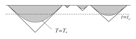
FIG. 1.: A conformal diagram of bubbles nucleating in an inflating background. The shaded regions of spacetime inside the bubbles are thermalized. The thermalization surfaces are the boundaries of these regions. They have an infinite $3$-volume which can be regularized by introducing a cutoff hypersurface $t=t_{c}$ and keeping only the part of the volume below this hypersurface.

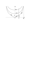
FIG. 2.: Geometry of the bubble interior.

FIG. 3.: The shape of the potential $V_{0}(\sigma)$ in Eq. (49).

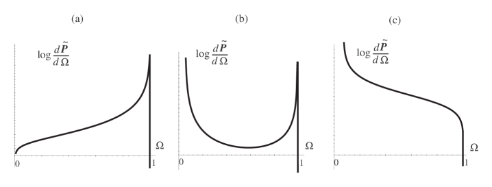
FIG. 4.: Probability distribution $d\tilde{{\cal{P}}}(\Omega)/d\Omega$ with $\phi_{\max}^{2}/\phi_{*}^{2}=100$, shown logarithmically up to a normalization. (a): $\mu=0.01$. The peak at $\Omega\approx 1$ is extremely sharp; the ratio of the values at $\Omega=.99$ and at $\Omega=0$ is $\sim\exp 20$, while the peak value differs from that at $\Omega=0$ by a factor of $\sim\exp\left(25000\right)$. (b): $\mu=0.5$, there are two local maxima near $\Omega=0$ and $\Omega=1$. (c): $\mu=2$. The function monotonically decreases. The maximum value at $\Omega=0$ differs from a typical intermediate value ($\Omega\sim 1/2$) by a factor of $\sim\exp\left(60\right)$.

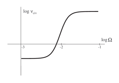
FIG. 5.: Dependence of $\nu_{\text{c}iv}$ on $\Omega$ for $\bar{\delta}=10^{-2}$. The ratio of the maximum and the minimum values is $\sim\exp\bar{\delta}^{-2}$. The origin on the vertical axis is arbitrary.

FIG. 6.: Probability distribution $d{\cal{P}}/d\Omega$, shown logarithmically up to a normalization, in the three cases corresponding to Fig. 4a-c. The parameter values are the same as those in Figs. 4, 5.

REFERENCES

-
[1]
For a review of inflation, see, e.g., A. D. Linde, Particle Physics and Inflationary Cosmology (Harwood Academic, Chur,
Switzerland, 1990); K. A. Olive, Phys. Rep. 190, 307 (1990).
-
[2]
J. R. Gott, III, Nature (London) 295, 304 (1982);
J. R. Gott, III and T. Statler, Phys. Lett. 136B, 157 (1984).
-
[3]
M. Bucher, A. S. Goldhaber, and N. Turok, Phys. Rev. D
52, 3314 (1995); M. Bucher and N. Turok, Phys. Rev. D 52, 5538
(1995).
-
[4]
T. Tanaka and M. Sasaki, Phys. Rev. D 50, 6444
(1994); K. Yamamoto, T. Tanaka and M. Sasaki, Phys. Rev. D 51, 2968
(1995).
-
[5]
A. D. Linde, Phys. Lett. B 351, 99 (1995); A. D.
Linde and A. Mezhlumian, Phys. Rev. D 52, 6789 (1995).
-
[6]
J. Garriga, preprint gr-qc/9602025; J. Garcia-Bellido,
preprint astro-ph/9510029.
-
[7]
A. Vilenkin, Phys. Rev. Lett. 74, 846 (1995).
-
[8]
B. Carter, in I.A.U. Symposium, vol. 63, ed. by
M. S. Longair (Reidel, Dordrecht, 1974).
-
[9]
B. J. Carr and M. J. Rees, Nature 278, 605 (1979).
-
[10]
J. Barrow and F. Tipler, The Antropic
Cosmological Principle (Clarendon Press, Oxford, 1986).
-
[11]
A. D. Linde, Particle Physics and Inflationary Cosmology
(Harwood Academic, Chur, 1990).
-
[12]
J. Leslie, Mind 101, 521 (1992).
-
[13]
The thermalization temperature is a convenient reference
point, but of course this choice is arbitrary, and one can use any other
reference temperature.
-
[14]
A. D. Linde, D. A. Linde, and A. Mezhlumian, Phys. Rev. D
49, 1783 (1994).
-
[15]
J. Garcia-Bellido, A. D. Linde, and D. A. Linde, Phys. Rev. D
50, 730 (1994).
-
[16]
A. Vilenkin, Phys. Rev. D 52, 3365 (1995).
-
[17]
S. Winitzki and A. Vilenkin, Phys. Rev. D 53,
4298 (1996).
-
[18]
It should be noted that the requirement of
time-reparametrization invariance alone does not fix a unique regularization
procedure. In fact, Linde and Mezhlumian [31] suggested a
generalization of the -prescription in which the co-moving volume
is replaced by a weighted volume , where is the physical volume and is a dimensionless parameter. Although all regularizations belonging to
this one-parameter family are time-reparametrization invariant, it was
argued in [17] that the original -prescription
(which corresponds to ) has some important advantages: (i) unlike
regularizations with , it can be applied to arbitrary inflaton
potentials, and (ii) it gives the “correct” answer in some cases where a
certain result is expected on intuitive grounds. We shall, therefore, adopt
the original -prescription in this paper and only briefly comment
on the results one would obtain from the modified prescriptions in
Sec. VII.
-
[19]
For a recent review of this stochastic approach to
inflation, see [14].
-
[20]
The function is rather
complicated,
Its explicit form will not be useful for us, and we can use the linear fit (36) to visualize its behavior.
-
[21]
As we noted before [18], the regularization
procedure of [16] which we use here is not unique, and a
set of alternative prescriptions depending on a parameter was proposed
in [31]; the original prescription is obtained for .
Analogous calculations can be performed using the alternative procedure. For
very small positive or negative satisfying , the modified Eq. (42) is
For larger negative satisfying , it becomes
-
[22]
F. C. Adams, Phys. Rev. D 48, 2800 (1993).
-
[23]
One can compare the probability distribution for obtained using alternative regularization procedures [18]
parametrized by with that in the case. The relevant formulae for
the thermalized volumes are given above in footnote [21]. The
allowed range of is , where is given by (54). The behavior of the distribution is similar to the case,
with maxima at and depending on the value of ,
but the values of separating different regimes become -dependent.
For large negative that satisfy , the peak is always at , whereas for small in the interval there are values of for which the peak is at .
-
[24]
The spectrum of density fluctuations is also -dependent, but this dependence is negligible on scales small compared to
the curvature radius of the bubble. This range of scales includes the
galactic scale, except for very small values of . Since drops exponentially fast as is
decreased, we expect that our conclusions will not be substantially modified
by taking into account the -dependence of the fluctuation spectrum.
-
[25]
It should be emphasized that our evaluation of can serve only as a very rough estimate. In
particular, for very low values of , galaxies are formed at a high
redshift (), and their properties may be very different
from those observed in our part of the universe. For example, a higher gas
density in the galaxy can affect the rate of star formation, and thus the
number of inhabitable stellar systems.
-
[26]
G. Steigman and J. E. Felten, Space Science Reviews
74, 245 (1995); A. D. Linde and A. Mezhlumian, in Ref. [5].
-
[27]
S. Weinberg, Phys. Rev. Lett. 59, 2607 (1987).
-
[28]
G. Efstathiou, M.N.R.A.S. 274, L73 (1995).
-
[29]
A. Vilenkin, in “Cosmological Constant and the Evolution
of the Universe”, ed. by K. Sato, T. Suginohara, and N. Sugiyama (Universal
Academy Press, Tokyo, 1996).
-
[30]
V. A. Berezin, V. A. Kuzmin, I. I. Tkachev, Phys. Lett. 120B,
91 (1983); Phys. Rev. D 36, 2919 (1987); also in Quantum Gravity, ed.
by M. A. Markov, V. A. Berezin and V. P. Frolov (World Scientific,
Singapore, 1985), p.781; R. Basu, A. H. Guth, and A. Vilenkin, Phys. Rev. D
44, 320 (1991).
-
[31]
A. D. Linde and A. Mezhlumian, Phys. Rev. D 53,
4267 (1996).