Abstract

We investigate how the qualitative structure of Doppler peaks in the angular power spectrum of the cosmic microwave anisotropy is affected by basic assumptions going into theories of structure formation. We define the concepts of “coherent” and “incoherent” fluctuations, and also of “active” and “passive” fluctuations. In these terms inflationary fluctuations are passive and coherent while topological defects are active incoherent fluctuations. Causality and scale invariance are shown to have different implementations in theories differing in the above senses. We then extend the formalism of Hu and Sugiyama to treat models with cosmic defects. Using this formalism we show that the existence or absence of secondary Doppler peaks and the rough placing of the primary peak are very sensitive to the fundamental properties defined. We claim therefore that even a rough measurement of the angular power spectrum $C_{l}$ shape at $100<l<1500$ ought to tell us which are the basic ingredients to be used in the right structure formation theory. We also apply our formalism to cosmic string theories. These are shown to fall into the class of active incoherent theories for which one can robustly predict the absence of secondary Doppler peaks. The placing of the cosmic strings’ primary peak is more uncertain, but should fall in $l\approx 400-600$.

1 Introduction

The cosmic microwave background (CMB) promises to become one of the most successful bridges between theory and experiment in cosmology. As the body of experimental data continues to grow[1], theorists are evaluating the impact of this data on the two major paradigms for cosmic structure formation: inflation [2] and topological defects [3]. The so-called Doppler peaks, in particular, have attracted great interest. They consist of a system of oscillations, known to be present for most inflationary models, in the CMB angular power spectrum $C_{l}$ at $100<l<1500$.

The Doppler peaks’ height and position have been extensively studied in inflationary scenarios [6], a context in which they can be used to fix with some accuracy combinations of cosmological parameters [7]. Although there has been some work on defect models [8, 9, 10], progress on defect Doppler peak predictions has been slow (see however [11, 12, 13]). In two recent letters [13, 19], we have claimed that regardless of the remaining quantitative uncertainties, one could expect dramatic qualitative differences between defect and inflationary Doppler peaks. In summary, we found two types of exotic behaviour. Firstly we found that defect Doppler peaks may be obtained from the inflationary ones by an additive shift in $l$. The shift value is roughly proportional to the inverse of the defect scaling coherence length. Only very large defects, on the verge of violating causality, apply a zero shift. We also found that defects should always soften the secondary Doppler oscillations, the more so the larger the additive shift they apply (the smaller their coherence length). Only “zero-shift” defects (placing the peaks on the inflationary positions) induce a negligible softening. If the main peak is at the isocurvature position one should not obtain more than an undulation. For a smaller coherence length (main peak to the right of the isocurvature position) the secondary peaks should be completely erased. These two types of phenomena are unheard of in inflationary scenarios. Putting aside “zero-shift” defects, we then claimed that measuring the qualitative features of the $C_{l}$ spectrum at $100<l<1500$ should decide between inflation and defects on fairly general grounds.

In this paper we explain in more detail the formalism outlined in [19], and present our findings in a more systematic form. As in [19] we focus on the basic assumptions of inflationary and defect theories in order to isolate the contrasting properties which alone determine the broad Doppler peak features (Section 3). We come up with two concepts: the concept of active and passive perturbations, and the concept of coherent and incoherent perturbations. In terms of these inflationary fluctuations are passive and coherent. Topological defects are active incoherent fluctuations. Causality and scale invariance are shown to have different implementations in theories differing in the above senses. These two concepts then allow us to write down a Hu and Sugiyama (H+S) type of formalism [4] tailored for cosmic defects (Sections 2 and 4). A number of simplifications apply, but one also needs to extend the existing work in two ways. Firstly, the way in which averages are taken has to be modified for incoherent perturbations. Two approximations may be useful: the coherent and the totally incoherent approximations. The factors controlling the applicability of these approximations are spelled out in Section 5.4. Secondly the H+S formalism cannot account for radiation backreaction, that is, for the radiation itself acting as a source for its own driving force. Causality, in defect theories, requires the existence of a large scale nonignorable radiation white noise-spectrum. This leads to a backreaction effect which can never be neglected. In Section 3.1.2 we show how to solve this problem.

We then apply our formalism in two types of study. In Section 5 we perform a qualitative analysis of defect Doppler peaks for a generic defect. We explain in more detail the results concerning the position of the primary peak and structure of secondary oscillations published in [19] and highlighted above. We go beyond the coherent and totally incoherent approximations. We also explicitly translate into $C_{l}$ spectra arguments initially developed in terms of the photons’ energy power spectrum at last scattering.

On a different front we target cosmic strings (Section 6). By using results from a cosmic string simulation we show that regardless of uncertainties one can safely predict that strings do not exhibit secondary oscillations. We also argue that the totally incoherent approximation is applicable to cosmic strings, and solve the full H+S algorithm in this approximation. The cosmic string (single) Doppler peak is shown to be in the region $l\approx 400-600$. Our simulation and formalism uncertainties do not yet allow us to make any prediction concerning the peak’s height relative to the low $l$ plateau.

2 Review of the Hu and Sugiyama formalism

We start by highlighting results in [4] of which we shall make use. The CMB photons are described by the brightness function $\Theta({\bf x},\mu,\eta)$, defined as the brightness temperature of photons moving in the direction $\mu$ at point ${\bf x}$ and time $\eta$. The brightness function satisfies the Boltzmann equation, which may be solved by expanding $\Theta({\bf x},\mu,\eta)$ in Fourier modes in space and Legendre polynomials in angle. The resulting components $\Theta_{l}(k,\eta)$ satisfy an infinite hierarchy of ODE’s, usually truncated and solved on a computer by a so-called Boltzmann code. The angular power spectrum $C_{l}$ can be obtained from the $\Theta_{l}(k,\eta)$ today ($\eta=\eta_{0}$) by using

$$C_{l}=\int_{0}^{\infty}dkk^{2}{\langle|\Theta_{l}(k,\eta_{0})|^{2}\rangle}\;.$$ (1)

where the brackets denote ensemble averages. In the analytical framework developed in [4], rather than making use of a Boltzmann code, evolution is split into three regimes for which analytical solutions are found: tight-coupling, recombination, and free-streaming. The idea is that before recombination photons are sufficiently tightly coupled to behave like a perfect fluid. For a perfect fluid the infinite series $\Theta_{l}(k,\eta)$ reduces to two non-vanishing components: the monopole $\Theta_{0}$ (related to the fluid energy density), and the dipole (related to its velocity). These satisfy perturbed perfect fluid equations, which can be analytically solved using the WKB approximation scheme. After recombination the photons free stream towards us. Although the infinite series $\Theta_{l}(k,\eta)$ is now required to describe the photons an exact solution for its evolution can be written. In between the two epochs there is recombination. If recombination were instantaneous one could simply glue together the two solutions. However this is never the case. The effects of finite recombination time can nevertheless be included in the form of a damping factor $D(k)$, describing Silk damping, an algorithm for which is supplied in [4]. A new paper by Battye has recently suggested some potentially important corrections to this method [5]. The corrections could raise the overall amplitude at small scales, but are unlikely to affect the presence or absence of the Doppler peaks, which we address here.

2.1 Free streaming

The free-streaming solution is approximately

$$\Theta_{l}(k,\eta_{0}) \approx [\Theta_{0}+\Psi](k,\eta_{*})j_{l}(k\Delta\eta_{*})+\Theta_{1}(k,\eta_{*}){lj_{l-1}(k\Delta\eta_{*})-(l+1)j_{l+1}(k\Delta\eta_{*})\over 2l+1}$$ (2)

$$+{\int^{\eta_{0}}_{\eta_{*}}}[{\dot{\Psi}}-{\dot{\Phi}}]j_{l}(k\Delta\eta)d\eta$$

where $\eta_{*}$ is the conformal time at last scattering, $\Delta\eta=\eta_{0}-\eta$, $\Delta\eta_{*}=\eta_{0}-\eta_{*}$, and $\Phi$ and $\Psi$ are the scalar gauge-invariant potentials (essentially the Newtonian potential on subhorizon scales). The first two terms represent the free streaming of spatial perturbations (of scale $k$) at last scattering into angular temperature fluctuations (of scale $l$) here and now. The first term is the free streaming projection of spatial fluctuations in the photon energy density (identified as $\Theta_{0}+\Psi$), and the second term the projection of fluctuations in the photons’ velocity (Doppler effect). The projectors are Bessel functions and peak at $l\approx k\Delta\eta_{*}$, but with some spread. Hence oscillations in the power spectra of $\Theta_{0}+\Psi$ and $\Theta_{1}$ at last scattering are translated into oscillation in the $C_{l}$ spectrum, but these always appear smoothed in the $C_{l}$. It is pointed out in [4] that the projector of the monopole term is more peaked than the projector of the dipole. Hence oscillations in the power spectrum of the monopole $\Theta_{0}$ at last scattering will be less smoothed out in the $C_{l}$ spectrum than oscillations in the dipole $\Theta_{1}$. In addition to the first two terms there is the Integrated Sachs Wolf (ISW) term, accounting for perturbations induced on photons in free flight after last scattering by non-conservative gravitational potentials.

2.2 Tight coupling

The equations ruling the photon fluid during tight coupling are:

$${\dot{\Theta}_{0}} = -{k\over 3}\Theta_{1}-{\dot{\Phi}}$$

$${\dot{\Theta}_{1}} = -{\dot{R}\over 1+R}\Theta_{1}+{k\over 1+R}\Theta_{0}+k\Psi\;,$$ (3)

where $R={3\over 4}{\rho_{b}\over\rho_{\gamma}}$ is the scale factor normalized to $3/4$ at photon-baryon equality. In this regime the baryons’ density contrast $\Delta_{b}$ and velocity $V_{b}$ satisfy the conditions

$${\dot{\Delta}_{b}} = {3\over 4}{\dot{\Delta}_{\gamma}}$$ (4)

$$V_{b} = V_{\gamma}\;,$$ (5)

where the photons’ density contrast $\Delta_{\gamma}$ and velocity $V_{\gamma}$ are to be found from

$$V_{\gamma} = \Theta_{1}$$ (6)

$$\Delta_{\gamma} = 4{\left(\Theta_{0}+h{\Theta_{1}\over k}\right)}\;.$$ (7)

We shall assume here that the main dynamical components are the photons and a defect component (and to a minor extent the baryons). Therefore we set the CDM density contrast $\Delta_{c}$ to zero. We also assume that Eqn.(4) can be integrated into $\Delta_{b}=(3/4)\Delta_{\gamma}$, that is, there are no entropy perturbations. These assumptions are not a requirement for the work to be presented, but are merely a simplification.

It may now happen that the potentials driving the fluid are external, or at any rate, known a priori. If this is the case then a WKB solution may be found for the monopole and dipole terms. For large $k$ (say $k>0.08h^{3}$) this is

$$[{\hat{\Theta}}_{0}+\Psi](\eta_{*}) = [\Psi-\Phi](\eta_{*})+{1\over(1+R_{*})^{1/4}}\bigg{(}[\cos{kr_{s}(\eta_{*})}+J(0)\sin{kr_{s}(\eta_{*})}][{\Theta}_{0}+\Psi](0)+I(\eta_{*})\bigg{)}$$ (8)

$${\hat{\Theta}}_{1}(\eta_{*}) = {{\sqrt{3}}\over(1+R_{*})^{3/4}}\Bigg{(}[1+J(\eta_{*})J(0)][{\Theta}_{0}+\Psi](0)\sin{kr_{s}(\eta_{*})}$$ (9)

$$+ [J(\eta_{*})-J(0)][{\Theta}_{0}+\Psi](0)\cos{kr_{s}(\eta_{*})}$$

$$+ J(\eta_{*})I(\eta_{*})-{k\over{\sqrt{3}}}{\int_{0}^{\eta_{*}}}d\eta\Phi(\eta)G(\eta)\cos[kr_{s}(\eta_{*})-kr_{s}(\eta)]\Bigg{)}$$

with

$$I(k,\eta) = {k\over{\sqrt{3}}}{\int_{0}^{\eta}}d\eta^{\prime}\Phi(\eta^{\prime})G(\eta^{\prime})\sin[kr_{s}(\eta)-kr_{s}(\eta^{\prime})]$$ (10)

$$G(k,\eta) = (1+R)^{-1/4}{\left(1-(1+R){\Psi\over\Phi}+{3{\ddot{R}}\over 4k^{2}}-J^{2}\right)}$$ (11)

$$J(k,\eta) = {{\sqrt{3}}\over 4k}{{\dot{R}}\over{\sqrt{1+R}}}$$ (12)

and where $r_{s}(\eta)$ is the sound horizon

$$r_{s}(\eta)={1\over{\sqrt{3}}}\int^{\eta}_{0}d\eta^{\prime}{1\over{\sqrt{1+R}}}\;.$$ (13)

For small $k$ (say $k<0.08h^{3}$) one may simply set $R=0$ in the solutions given above.

The gauge-invariant scalar potentials driving this system may be obtained from Einstein’s equations [21]

$$k^{2}\Phi = 4\pi{\left(a^{2}\rho\Delta_{T}+\rho^{s}+3hv^{s}\right)}$$ (14)

$$\Phi+\Psi = -8\pi{\left(a^{2}{p\Pi\over k^{2}}+\Pi^{s}\right)}$$ (15)

where $a$ is the scale factor, $h=\dot{a}/a$, $\rho$ ($\Delta_{T}$) is the total matter density (density contrast), and $p\Pi/k^{2}$ is simply related to the nearly vanishing quadrupole of the photon and neutrino fluctuations. In the tight coupling regime one may set $\Pi=0$ in a first approximation, and the total density contrast may be written as

$$\rho\Delta_{T}=\rho_{b}\Delta_{b}+\rho_{\gamma}\Delta_{\gamma}=\rho_{\gamma}\Delta_{\gamma}(1+R)$$ (16)

from Equation 4. We have included a defect component with stress-energy tensor $\Theta_{\mu\nu}$ given by

$$\Theta_{00} = \rho^{s}$$

$$\Theta_{0i} = k_{i}v^{s}$$

$$\Theta_{ij} = p^{s}\delta_{ij}+(k_{i}k_{j}-{1\over 3}\delta_{ij}k^{2})\Pi^{s}$$ (17)

as in [22] (but rewritten in terms of $\Theta_{\mu\nu}$ rather than $\Theta^{\mu}_{\nu}$). Equations (14) and (15) have the advantage of being elliptical, thus allowing a simple connection between sources and potentials. They form a complete set as long as the sources are conserved. For the defects this means:

$${\dot{\rho}}^{s}+h(3p^{s}+\rho^{s})+k^{2}v^{s} = 0$$ (18)

$${\dot{v}}^{s}+2hv^{s}-p^{s}+{2\over 3}k^{2}\Pi^{s} = 0\;.$$ (19)

3 Topological defects contrasted with inflation

We now focus on the basic assumptions of inflationary and defect theories and isolate the contrasting properties. This will allow us to write down a defect tailored Hu and Sugiyama formalism. We shall use the resulting formalism both in general arguments concerning defect scenarios, and in rigorous calculations for particular defects. We define the concepts of active and passive perturbations, and of coherent and incoherent perturbations. In terms of these concepts inflationary perturbations are passive coherent perturbations. Defect perturbations are active perturbations more or less incoherent depending on the defect.

3.1 Active and passive perturbations, and their different perceptions of causality and scaling

The way in which inflationary and defect perturbations come about is radically different. Inflationary fluctuations were produced at a remote epoch, and were driven far outside the Hubble radius by inflation. The evolution of these fluctuations is linear (until gravitational collapse becomes non-linear at late times), and we call these fluctuations “passive”. Also, because all scales observed today have been in causal contact since the onset of inflation, causality does not strongly constrain the fluctuations which result. In contrast, defect fluctuations are continuously seeded by defect evolution, which is a non-linear process. We therefore say these are “active” perturbations. Also, the constraints imposed by causality on defect formation and evolution are much greater than than those placed on inflationary perturbations.

3.1.1 Active and passive scaling

The notion of scale invariance has different implications in these two types of theory. For instance, a scale invariant gauge-invariant potential $\Phi$ with dimensions $L^{3/2}$ has a power spectrum

$$P(\Phi)=\langle|\Phi_{\bf k}|^{2}\rangle\propto k^{-3}$$

in passive theories (the Harrison-Zeldovich spectrum). This results from the fact that the only variable available is $k$, and so the only spectrum one can write down which has the right dimensions and does not have a scale is the Harrison-Zeldovich spectrum. The situation is different for active theories, since time is now a variable. The most general counterpart to the Harrison-Zeldovich spectrum is

$$P(\Phi)=\eta^{3}F_{\Phi}(k\eta)$$ (20)

where $F_{\Phi}$ is, to begin with, an arbitrary function of $x=k\eta$. All other variables may be written as a product of a power of $\eta$, ensuring the right dimensions, and an arbitrary function of $x$. Inspecting all equations it can be checked that it is possible to do this consistently for all variables. All equations respect scaling in the active sense.

3.1.2 Causality constraints on active perturbations

Moreover, active perturbations are constrained by causality, in the form of integral constraints [14, 15]. These consist of energy and momentum conservation laws for fluctuations in an expanding Universe. The integral constraints can be used to find the low $k$ behaviour of the perturbations’ power spectrum, assuming their causal generation and evolution [20]. Typically it is found that the causal creation and evolution of defects requires that their energy $\rho^{s}$ and scalar velocity $v^{s}$ be white noise at low $k$, but that the total energy fluctuations’ power spectrum is required to go like $k^{4}$. To reconcile these two facts one is forced to consider the compensation. This is an underdensity in the matter-radiation energy density with a white noise low $k$ tail, correlated with the defect network so as to cancel the defects’ white-noise tail.

We first derive directly the low $k$ behaviour of all variables in our problem. For low $k$ one may set $R=0$, $\Delta_{T}\approx\Delta_{\gamma}\approx 4\Theta_{0}$, and solve equations (3) coupled to (14) and (15) to find

$$\Theta_{0} = -4\pi{\rho^{s}+3hv^{s}\over k^{2}+6h^{2}\Omega_{\gamma}}$$ (21)

$$a^{2}\rho\Delta_{T} = -6h^{2}{\rho^{s}+3hv^{s}\over k^{2}+6h^{2}\Omega_{\gamma}}$$ (22)

$${\cal U}=a^{2}\rho\Delta_{T}+\rho^{s}+3hv^{s} = {k^{2}(\rho^{s}+3hv^{s})\over k^{2}+6h^{2}\Omega_{\gamma}}$$ (23)

$$\Phi=-\Psi = 4\pi{\rho^{s}+3hv^{s}\over k^{2}+6h^{2}\Omega_{\gamma}}$$ (24)

where $\Omega_{\gamma}=\rho_{\gamma}/\rho$, and we have used $3h^{2}=8\pi\rho$. This solution is in fact valid for all values of $k$ for which the dipole $\Theta_{1}$ is negligible. The lack of superhorizon correlations in the defect network requires the power spectrum $P(\rho^{s})$ to have a white noise low $k$ tail. Energy conservation Eqn. (18) requires that $v^{s}$ also have a white noise low $k$ tail. Equations (21) and (22) show the emergence of the compensation: a necessary low $k$ white-noise tail in the radiation power spectrum exactly anticorrelated with the defects’ tail. The quantity to be cancelled is $\rho^{s}+3hv^{s}$, and not just $\rho^{s}$. The density forced to have a $k^{4}$ power spectrum is ${\cal U}$, as shown by (23), and not just a combination of $\Delta_{T}$ and $\rho^{s}$. This is precisely the source term for the potential $\Phi$ which must therefore be white-noise on large scales. Since isotropy requires $\Pi^{s}$ and $p\Pi/k^{2}$ to be constant for small $k$, the Einstein equations imply that scaling active perturbations produce scaling gauge-invariant potentials, which must be white-noise on large scales. In particular $P(\Psi-\Phi)=F(k\eta)\eta^{3}$, with $F(0)$ a non-zero constant. For most realistic defects $x^{4}F(x)$ will then have a single peak, located at a value of $x\equiv x_{c}$ corresponding roughly to the “coherence scale” of the defect in question. We will see that the place and thickness of the peak in $x^{4}F(x)$ are deciding features for the Doppler peaks induced by active perturbations.

These results can be understood by means of integral constraints. Although gauge-invariant in their initial formulation, integral constraints have been applied to defects in terms of the gauge dependent energy-momentum pseudo-tensor of [17, 18]. Here we go back to their original formulation, and rewrite the defect integral constraints in terms of gauge-invariant variables. If a given perturbation has a compact support then according to [14] the following quantity must be conserved

$${\cal E}=\int dV(\delta T^{0}_{0}-x^{i}h\delta T^{0}_{i})\;.$$ (25)

It can be checked that the density ${\cal U}=(\delta T^{0}_{0}-x^{i}h\delta T^{0}_{i})$ is gauge invariant under transformations which go to zero outside the perturbation boundary. Since the Universe is unperturbed outside this boundary, setting all $local$ perturbation variables to zero in this region is a natural gauge restriction. Assuming a purely scalar perturbation, and integrating the second term in (25) by parts the density ${\cal U}$ can then be written as

$${\cal U}=a^{2}\rho\Delta_{T}+\rho^{s}+3hv^{s}$$ (26)

which is precisely the source term in (14) and the quantity given in (23). Using similar arguments it can be shown that the other three integral constraints concern integrals of the form $\int dV\,x^{i}{\cal U}$. Using these two constraints it was shown in [20] that if the perturbation field is the sum of individual contributions with a compact support and which are uncorrelated beyond a certain length, then the power spectrum of the total ${\cal U}$ field has to be bound by $k^{4}$ as $k\rightarrow 0$. This is precisely what we have found by studying directly the low $k$ behaviour of the tight-coupled equations.

The compensation can be implemented in the form of a compensation factor [24]. In our language this means postulating an equation of state for $\Delta_{T}$ of the form

$${\cal U}=a^{2}\rho\Delta_{T}+\rho^{s}+3hv^{s}=\gamma_{c}(\rho^{s}+3hv^{s})$$ (27)

Usually one writes

$$\gamma_{c}={1\over 1+{\left({\chi_{c}\over x}\right)}^{2}}$$ (28)

where $\chi_{c}$ is the compensation scale. Equation (23) suggests that if $h\eta=\alpha$ then $\chi_{c}={\sqrt{6\Omega_{\gamma}}}\alpha$. Then $\chi_{c}\approx 2.45$ in the radiation era. In work in preparation [23] we show that $\gamma_{c}$ is more than just a “fudge” factor. The radiation backreaction is indeed dominated by a factor of the form of $\gamma_{c}$. However, secondary radiation backreaction effects occur. A dipole driven monopole wave, with $k^{4}$ large scale behaviour and so not required by causality, is of particular relevance. It always acts so as to push the compensation scale further inside the horizon. Hence we consider a range of $\chi_{c}$ going over its limiting value of 2.45.

3.2 Coherent, incoherent, and totally incoherent perturbations

Active perturbations may also differ from inflation in the way “chance” comes into the theory. Randomness occurs in inflation only when the initial conditions are set up. Time evolution is linear and deterministic, and may be found by evolving all variables from an initial value equal to the square root of their initial variances. By squaring the result one obtains the variables’ variances at any time. Formally this results from unequal time correlators of the form

$${\langle\Phi({\bf k},\eta)\Phi({\bf k^{\prime}},\eta^{\prime})\rangle}=\delta({\bf k}-{\bf k^{\prime}})\sigma({\Phi}(k,\eta))\sigma({\Phi}(k,\eta^{\prime})),$$ (29)

where $\sigma$ denotes the square root of the power spectrum $P$. In defect models however, randomness may intervene in the time evolution as well as the initial conditions. Although deterministic in principle, the defect network evolves as a result of a complicated non-linear process. If there is strong non-linearity, a given mode will be “driven” by interactions with the other modes in a way which will force all different-time correlators to zero on a time scale characterized by the “coherence time” $\tau_{c}(k,\eta)$. Physically this means that one has to perform a new “random” draw after each coherence time in order to construct a defect history [13]. The counterpart to (29) for incoherent perturbations is

$${\langle\Phi({\bf k},\eta)\Phi({\bf k^{\prime}},\eta^{\prime})\rangle}=\delta({\bf k}-{\bf k^{\prime}})P({\Phi}(k,\eta),\eta^{\prime}-\eta)\;.$$ (30)

For $|\eta^{\prime}-\eta|\equiv|\Delta\eta|>\tau_{c}(k,\eta)$ we have $P({\Phi}(k,\eta),\Delta\eta)=0$. For $\Delta\eta=0$, we recover the power spectrum $P({\Phi}(k,\eta),0)=P({\Phi}(k,\eta))$. If there is active scaling we have seen that $P({\Phi}(k,\eta))=\eta^{3}F_{\Phi}(x)$. Also the correlation

$${\rm cor}(\Phi(k,\eta),\Phi(k,\eta^{\prime}))={{\langle\Phi(k,\eta)\Phi(k,\eta^{\prime})\rangle}\over\sigma(\Phi(k,\eta))\sigma(\Phi(k,\eta^{\prime}))}$$

must be a function of only $x=k\eta$ and $x^{\prime}=k\eta^{\prime}$. Let’s call it ${\cal C}_{\Phi}(x,x^{\prime})$. Since there is no time translational invariance, this function is not necessarily dependent only on $x-x^{\prime}$. Hence, if there is active scaling, we can write

$${\langle\Phi({\bf k},\eta)\Phi({\bf k^{\prime}},\eta^{\prime})\rangle}=\delta({\bf k}-{\bf k^{\prime}})(\eta^{3}F_{\Phi}(x))^{1/2}(\eta^{\prime 3}F_{\Phi}(x^{\prime}))^{1/2}{\cal C}_{\Phi}(x,x^{\prime}).$$ (31)

Detailed understanding of the effects of incoherence on the structure of Doppler peaks requires knowledge of the coherence function ${\cal C}(x,x^{\prime})$. However two approximation schemes have been implemented. In one effective coherence was assumed so that ${\cal C}(x,x^{\prime})=1$. This was done in calculations for texture models [11, 12], where coherent statistics were assumed. In another [13] it was assumed that

$${\langle\Phi({\bf k},\eta)\Phi({\bf k^{\prime}},\eta^{\prime})\rangle}=\delta({\bf k}-{\bf k^{\prime}})\delta(\eta-\eta^{\prime})P_{r}({\Phi}(k,\eta)),$$ (32)

in which

$$P_{r}({\Phi}(k,\eta))={{\int}}\,d\Delta\eta P({\Phi}(k,\eta),\Delta\eta)$$ (33)

is the time-integrated power spectrum [24]. This is far less naive than just setting ${\cal C}(x,x^{\prime})=\delta(x-x^{\prime})$ in (31) and draws on the methods of [24]. It should be a good approximation whenever convolving $P({\Phi}(k,\eta),\Delta\eta)$ with functions which vary slowly at the scale of $\tau_{c}(k,\eta)$. Clearly both approximations have drawbacks, and it is up to detailed calculations to decide which of the two approximations is better, if any, in each particular situation.

We shall label as coherent, incoherent, and totally incoherent the perturbations satisfying (29), (30), and (32) respectively. This feature changes the way the average $C^{l}$ are computed, resulting in a striking qualitative difference in the structure of Doppler peaks.

A comment should be added concerning the possibility of different coherence properties among the different components which act as sources for the potentials $\Phi$ and $\Psi$ (cf. Eqns. (14) and (15)). Indeed it could happen that say, radiation behaved coherently while defects behaved incoherently. In such a case the potentials coherence properties would naturally mix their sources coherence properties in a fashion easily predictable from Einstein’s equations. However, as we explain in Section 4.1, it is a good approximation to neglect the $a^{2}\rho\Delta_{T}$ contribution to the potentials except for the compensation. The compensation, on the other hand, is given by the large scale solution found in Section 3.1.2. It should be noted that Eqn.(22) applies for each realization, implying perfect correlation between defects and compensation. It follows that the compensation has the same coherence properties as the defect network. Therefore within the approximation spelled out further in Section 4.1, the potentials have the same coherence properties as the defects.

4 A defect-tailored Hu and Sugiyama formalism

In scenarios in which perturbations are driven by a topological defect network, a number of simplifications and extensions apply to the Hu and Sugiyama formalism. Making use of active scaling and the low $k$ constraints (21) to (24) one may prove that one may drop all but the convolution terms in (8) and (9). In fact they will be suppressed relative to the convolution terms by a factor of order $(\eta_{ph}/\eta_{*})^{3/2}$, where $\eta_{ph}$ is the conformal time of the phase transition. Then the multipoles $\Theta_{l}(k,\eta_{0})$ may be written in the simplified form

$$\Theta_{l}(k,\eta_{0}) = {\int_{0}^{\eta_{*}}}d\eta\,k\Phi(k,\eta)G(k,\eta){\left(D^{l}(k,\eta)+V^{l}(k,\eta)\right)}+$$ (34)

$$+ (\Psi-\Phi)(\eta_{*})j_{l}(k\Delta\eta_{*})+{\int_{\eta_{*}}^{\eta_{0}}}({\dot{\Psi}}-{\dot{\Phi}})j_{l}(k\Delta\eta)$$

with

$$D^{l}(k,\eta) = {j_{l}(k\Delta\eta_{*})\over{\sqrt{3}}(1+R_{*})^{1/4}}\sin(kr_{s}(\eta_{*})-kr_{s}(\eta))$$

$$V^{l}(k,\eta) = {lj_{l-1}(k\Delta\eta_{*})-(l+1)j_{l+1}(k\Delta\eta_{*})\over(2l+1)(1+R_{*})^{3/4}}\times$$ (35)

$$\times [J(\eta_{*})\sin(kr_{s}(\eta_{*})-kr_{s}(\eta))-\cos(kr_{s}(\eta_{*})-kr_{s}(\eta))]\;.$$

If one assumes coherence then one may simply compute the $\Theta_{l}(k,\eta_{0})$ with this formula, replacing every variable by the square root of its power spectrum. By squaring the result one then obtains ${\langle|\Theta_{l}(k,\eta_{0})|^{2}\rangle}$, providing the $C_{l}$ spectrum by means of (1). If the perturbation is incoherent then the H+S formalism must be modified at this step. For totally incoherent perturbations (imposing (32)) one has instead:

$$C_{l} = \int dk{\int_{0}^{\eta_{*}}}d\eta k^{4}P_{r}(\Phi(k,\eta)G(k,\eta)){\left({D^{l}(k,\eta)+V^{l}(k,\eta)}\right)}^{2}+$$ (36)

$$+ \int dkk^{2}P(\Psi-\Phi)(\eta^{*})j_{l}^{2}(k\Delta\eta_{*})+\int dkk^{3}{[V^{l}j_{l}(k\Delta\eta_{*})\sigma^{r}(\Phi G)\sigma^{r}(\Psi-\Phi)](\eta^{*})}$$

$$+ \int dk{\int_{\eta_{*}}^{\eta_{0}}}d\eta k^{2}P_{r}({\dot{\Psi}}-{\dot{\Phi}})j^{2}_{l}(k\Delta\eta)\;.$$

For incoherent perturbations the problem is always more complicated numerically, as one has to perform two integrals in time and one in $k$.

Even before performing any calculations one may expect striking differences between defects and inflationary Doppler peaks. For active perturbations the convolution terms dominate over the primordial terms in the monopole and dipole terms. Since the phase $kr_{s}(\eta_{*})$ enters differently in the primordial and convolution terms one may expect differences in the Doppler peaks’ position. Also, in obtaining the $C_{l}$ for coherent active perturbations one integrates an oscillatory function and then squares the result. Some oscillatory structure can always be expected in the $C_{l}$. For totally incoherent active perturbations, on the contrary, one simply integrates the square of an oscillatory function. This contains a DC level as well as an AC level. These will compete, leaving it up to other details of the incoherent perturbation to decide whether or not there are secondary oscillations. We will expand in great detail on these two points.

4.1 Possible loopholes

Eqns. (1), (2), (8), (9), (14), and (15) seem to imply that topological defects’ $C_{l}$ spectra may be analytically computed just from knowledge of the defect two-point functions

$${\langle\Theta_{\mu\nu}(\eta)\Theta_{\alpha\beta}(\eta^{\prime})\rangle}.$$ (37)

This includes knowledge of time-time correlators, and also cross-correlators involving different stress-energy components. However there are two loopholes in this statement which we now spell out.

In the H+S formalism one assumes that the potentials are external to the photon-baryon fluid, or at least, are known a priori. The defect potentials are indeed external, since defects evolve according to their own independent dynamics (the so-called stiff defect assumption [17]). However we know that we cannot neglect $\Delta_{\gamma}$ on large scales, as the compensation is of the same order of magnitude as the defect perturbations themselves. Since $\Delta_{\gamma}$ acts as a source for its own driving potentials we have a loophole in the formalism, as we cannot account for radiation backreaction effects. This is not necessarily a problem, as we have an explicit low $k$ solution for the radiation (Eqns. (21) to (24)). Hence we may account for the nonignorable radiation backreaction in the form of a factor $\gamma_{c}$, as in Eqn.(28). Thus we include radiation backreaction where it is required by causality, and ignore it otherwise. Many of the uncertainties in the backreaction may be mimicked by leaving $\chi_{c}$ as a free parameter. We shall see that the particular Doppler peak features we are interested in are insensitive to this uncertainty. In future work [23] we will write down solutions for the tight-coupling equations driven by a defect source, which incorporate exact radiation backreaction. These show that $\gamma_{c}$ is in fact the leading order backreaction effect. In another approach [25] we will simply solve the differential equations (3) directly. Although this approach can cope with the compensation exactly, it has the disadvantage of requiring a Monte-Carlo technique.

A second loophole concerns the measurement of the two-point correlators (37) from simulations. It may happen that we can only measure one term in the overall defect associated stress-energy. For instance a full account of cosmic string evolution requires consideration of evolution of tiny loops and the gravitational radiation they dissolve into. These are usually overlooked in string simulations. However it is extremely important to keep track of every defect stress-energy term, as one needs them all to ensure energy conservation, without which Eintein’s equations are not integrable. If however one assumes that the overlooked terms are a minor contribution to the total stress-energy tensor, then they can be neglected in our formalism. Equations (14) and (15) can be solved separately for every stress-energy component. If gravitational radiation is negligible then so are its induced potentials $\Phi$ and $\Psi$. This statement remains true even though one needs the gravitational radiation component to integrate the whole set of Einstein’s equations.

These loopholes concern calculations of $C_{l}$ spectra for concrete motivated defect scenarios (such as cosmic strings or textures). They do not affect the general analysis performed in Section 5.

5 Doppler peaks for a generic defect

We now undertake a qualitative general analysis of peak position and secondary oscillation strength in the monopole power spectrum at last scattering. We input qualitative perturbation features, as general as possible, for which we output only qualitative peak features. The idea is to find out which novelties in defect peak features are generic defect properties as opposed to mere accidents pertaining to particular defect models. Also we may learn when and why the coherent and totally incoherent approximations are too crude to be useful.

Figure 1: The dimensionless power spectrum of the monopole term $k^{3}P(\Theta_{0}+\Psi)(\eta_{*})$ plotted as a function of $k^{*}$ for adiabatic (line) and isocurvature (dashed) passive fluctuations.

The free-streaming solution (2) suggests interpreting $(\Theta_{0}+\Psi)(\eta_{*})$ as the intrinsic anisotropy $\delta_{\gamma}$, that is, the anisotropy due to photon energy density fluctuations at last scattering. This anisotropy has the sharpest free-streaming conversion from $k$ to $l$ and is responsible for the overall Doppler peak features. In particular the Doppler peak’s position and the structure of secondary oscillations may be inferred from the power spectrum $P(\delta_{\gamma})(\eta_{*})$. However it should be borne in mind that oscillations in $P(\delta_{\gamma})$ overestimate oscillations in the $C_{l}$. If we stick to low values of $\Omega_{b}h^{2}$ then the position and structure of the peaks is only mildly dependent on these parameters. In this Section we neglect this dependence altogether by implementing an approximation where $R=0$, $r_{s}(\eta)=\eta/{\sqrt{3}}$. This is a simplification for illustrative purposes and not a formalism requirement. Then, from (8), we have

$$(\Theta_{0}+\Psi)(\eta_{*})=(\Psi-\Phi)(\eta_{*})+{k\over{\sqrt{3}}}\int_{0}^{\eta_{*}}d\eta\,(\Phi-\Psi)\sin{{k(\eta_{*}-\eta)\over{\sqrt{3}}}}$$ (38)

If there is active scaling, in the sense of Eqn.(31), one has

$${\langle(\Psi-\Phi)(\eta)(\Psi-\Phi)(\eta^{\prime})\rangle}=(\eta^{3}F(x))^{1/2}(\eta^{\prime 3}F(x^{\prime}))^{1/2}{\cal C}(x,x^{\prime}).$$ (39)

with $x=k\eta$, $x^{\prime}=k\eta^{\prime}$. Here $F(x)$ is the structure function (as in [24]) or scaling factor (as in Eqn.(20)) of the potential $\Psi-\Phi$,

$$P(\Psi-\Phi)=\eta^{3}F(x)$$ (40)

and ${\cal C}$ is its coherence function. The dimensionless power spectrum $k^{3}P(\delta_{\gamma})(\eta_{*})$ is then only dependent on $x_{*}=k\eta_{*}$ and may be computed from

$$k^{3}P(\Theta_{0}+\Psi)(\eta_{*}) = x^{3}_{*}F(x_{*})-{2\over{\sqrt{3}}}(x_{*}^{3}F(x_{*}))^{1/2}{\int_{0}^{x_{*}}}dx\,{\cal C}(x,x_{*})(x^{3}F(x))^{1/2}{\sin{x_{*}-x\over{\sqrt{3}}}}+$$ (41)

$$+ {1\over 3}\int_{0}^{x_{*}}\int_{0}^{x_{*}}dx\,dx^{\prime}\,{\left((x^{3}F(x))^{1/2}{\sin{x_{*}-x\over{\sqrt{3}}}}\right)}{\left(x\rightarrow x^{\prime}\right)}{\cal C}(x,x^{\prime})$$

If we use a coherent approximation (${\cal C}=1$) this becomes

$$k^{3}P(\Theta_{0}+\Psi)(\eta_{*})={\left((x^{3}_{*}F(x_{*}))^{1/2}-{1\over{\sqrt{3}}}{\int_{0}^{x_{*}}}dx\,(x^{3}F(x))^{1/2}\sin{{x_{*}-x\over{\sqrt{3}}}}\right)}^{2}$$ (42)

If we use a totally incoherent approximation one has instead

$$k^{3}P(\Theta_{0}+\Psi)(\eta_{*})=x^{3}_{*}F(x_{*})+{1\over 3}{\int_{0}^{x_{*}}}dx\,x^{4}F_{r}(x)\sin^{2}{{x_{*}-x\over{\sqrt{3}}}}$$ (43)

in which $F_{r}$ is the structure function for the time-integrated power spectrum of $\Psi-\Phi$ as defined by (32) and (33):

$$P_{r}(\Psi-\Phi)=\eta^{4}F_{r}(x)$$ (44)

The rough peak structure in passive theories may be obtained by dropping all but the primordial terms [4], thereby ignoring sub-horizon processing. Thus for Harrison-Zeldovich initial conditions one has:

$$k^{3}P(\Theta_{0}+\Psi)(\eta_{*}) \propto {\cos^{2}{x_{*}\over{\sqrt{3}}}}$$ (45)

$$k^{3}P(\Theta_{0}+\Psi)(\eta_{*}) \propto {\sin^{2}{x_{*}\over{\sqrt{3}}}}$$ (46)

for adiabatic and isocurvature passive fluctuations. For reference we have plotted these spectra in Figure 1. The maxima are at scales $x^{*}_{m}/{\sqrt{3}}=m\pi$ and $x^{*}_{m}/{\sqrt{3}}=(m+1/2)\pi$, respectively. There are true zeros in the power spectrum, which get smoothed out into valleys in the $C_{l}$ spectrum. These valleys are further filled by the dipole, but since this is suppressed, the oscillatory structure survives. The free-streaming monopole projector is simply a Bessel function $j_{l}(x)$, which has its main peak at $x\approx l$. Then the peaks in $k^{3}P(\Theta_{0}+\Psi)(\eta_{*})$ will be converted into angular scales $l_{m}\approx(\eta_{0}/\eta_{*})x_{m}^{*}$. An improvement on this formula may be obtained by noticing that the peak of $j_{l}(x)$ is in fact at $x\approx l+0.8l^{1/3}$.

5.1 A representative generic defect

We now cut a representative section through the infinite dimensional defect parameter space. The physical inputs into (41) are the coherence function ${\cal C}(x,x^{\prime})$ and the potential structure function. Both may be obtained from the sources via Einstein’s equation:

$$k^{2}(\Phi-\Psi)=8\pi(a^{2}\rho\Delta_{T}+\rho^{s}+3hv^{s}+k^{2}\Pi^{s})$$ (47)

Then if $F_{\rho^{s}}$ is the defect energy structure function

$$P(\rho^{s})=F^{2}_{\rho^{s}}/\eta$$ (48)

one has

$$x^{4}F(x)=(8\pi)^{2}\gamma_{c}^{2}F^{2}_{\rho^{s}}\Gamma^{2}$$ (49)

in which we use a compensation of the form (27), and have assumed that the defect’s $v^{s}$ and $\Pi^{s}$ are related to its energy via equations of state, leading to the factor $\Gamma$. $F_{\rho^{s}}^{2}\Gamma^{2}$ must go to white noise at low $k$, and for realistic defects it falls-off like $1/x^{n}$ at large $k$. Then $F(x)$ must be white noise at low $x$, tailing off like $1/x^{n+4}$ at high $x$. $x^{4}F(x)$ will then have a peak at a turn-over scale close to $x_{c}\equiv 2\pi\eta/\xi_{c}$, where $\xi_{c}$ is approximately the coherence length of the defect (the wavelength where $F_{\rho^{s}}^{2}\Gamma^{2}$ switches from white noise to power law fall-off). This means that $x^{3}F(x)$ and $x^{4}F_{r}(x)$ will also have a peak, typically not very far off the peak in the potential source structure function $x^{4}F(x)$. Inspecting Eqns. 41, 42, and 43 we see that more than the exact form of the potential structure functions, it is the place and thickness of this peak that will determine the Doppler peak structure. For the purpose of the qualitative discussion to be carried out we then assume for definiteness that for our generic defect

$$F(x)=\exp{x^{2}\over 2\sigma^{2}}$$ (50)

placing the peak of $x^{4}F(x)$ at $x_{c}=2\sigma$. This form allows us to consider a one parameter family of structure functions for which both the peak position and the width are determined by the single parameter $\sigma$. In the familiar cases this “one scale” feature of the structure function is realistic, but it is worth noting that exotic cases could provide exceptions to the straightforward analysis which follows from (50). It is an important question of principle to know how small $x_{c}$ may be before causality is violated. The value $x_{c}\approx 2.7$ was suggested in [15]. Recently, a more systematic analysis of this question has been given by Turok[16] who gets similar results.

Strictly speaking the structure function (50) violates causality. ¿From (49) it implies a structure function for $\rho^{s}$ which once inverted into real space reveals vanishingly small, but not strictly zero superhorizon correlations. If one wants to be pedantic about this, one may simply set the real space structure function to zero outside the horizon, reinvert to Fourrier space, and find the corresponding modification to $F(x)$. Depending on how smoothly the cut-off is done a set of sub-dominant oscillations may or may not appear in the modified causal $F(x)$ (as stated in [16]). In any case, the correction in $F(x)$ is very small, and it certainly does not affect the integrals leading to the $C_{l}$ spectra needed for the sake of our argument. For this reason we shall ignore this detail in the rest of our discussion.

For a compensation satisfying (27) the compensation coherence time is the same as the defect coherence time. Hence the potential coherence function is also the defect coherence function. We will assume that our generic defect has a coherence function of the form

$${\cal C}(x,x^{\prime})=\exp{(x-x^{\prime})^{2}\over 2\tau_{c}^{2}}$$ (51)

in which the FWHM coherence time is given by $\theta_{c}\approx 2.35\tau_{c}$.

5.2 The peak position for active perturbations

Figure 2: Four potential source structure functions ($F(x)x^{4}$ where $F(x)$ is the potential structure function) and their corresponding spectra $k^{3}P(\Theta_{0}+\Psi)(\eta_{*})$ (dashed lines) assuming coherence. The continuous line in the bottom diagram represents a passive adiabatic spectrum. For a sufficiently small $\xi_{c}$ one obtains the adiabatic structure of peaks. As $\xi_{c}$ increases one may obtain the isocurvature peaks. However one cannot realistically push the peaks much further to the right without destroying the symmetry of the secondary peaks.

If the peak in $x^{4}F(x)$ is sufficiently thin, then from (41), (42), and (43), the monopole spectrum peaks will be at $x^{*}_{m}=(m-1/2)\pi{\sqrt{3}}+x_{c}$ for coherent, incoherent, and totally incoherent fluctuations. Then active perturbations merely apply a phase shift of value $x_{c}-\pi{\sqrt{3}}/2$ to an adiabatic type of spectrum (cf. Eqn. 45).

For $x_{c}\approx 2.7$ (not impossible, but probably unrealistic because it is very close to the smallest turnover point allowed by causality [15, 16]) the monopole peaks are at the adiabatic positions. As $x_{c}$ increases from the adiabatic position the peaks are shifted to smaller scales. For $x_{c}\approx 5.4$ they are out of phase with the adiabatic peaks (as in [11]). For $x_{c}>8.5$ the peaks start only in the adiabatic secondary peaks region. For standard values of $\Omega_{b}$ and $h$ these three cases would place the main “Doppler peak” at $l\approx 230$, $350$, and $500$, respectively. Therefore the placing of the peaks is not a generic feature of active fluctuations. Active perturbations simply add an extra parameter on which the Doppler peaks position is strongly dependent. In general we should expect that for the same $\Omega$, $\Omega_{b}$, and $h$, active perturbations will apply to the predicted CDM adiabatic peak position a shift of the form

$$l\rightarrow l+{\eta_{0}\over\eta^{*}}{\left(x_{c}-{\pi{\sqrt{3}}\over 2}\right)}$$ (52)

The secondary peaks’ separation is not changed, in a first approximation. This is to be contrasted with non-flat inflationary models where $C_{l}(\Omega=1)$ is taken into $C_{l\Omega^{-1/2}}$. The defect shift is additive whereas the low-$\Omega$ shift is multiplicative, a striking difference that should always allow us to distinguish between low $\Omega$ CDM and $\Omega=1$ high-$x_{c}$ defects.

If the peak in $x^{4}F(x)$ is thick then the issue of coherence comes into play but all we have said still applies if the perturbation is exactly coherent. This is illustrated in Fig. 2 using the generic model defined in Section 5.1. A formula for the peaks of $P(\Theta_{0}+\Psi)(k,\eta_{*})$ for more general structure functions of coherent active perturbations can be obtained by computing the structure function “primitives”:

$$F_{1}(x_{*}) = {\int^{x_{*}}_{0}}dx\,x^{3/2}{\sqrt{F(x)}}\cos(x/{\sqrt{3}})$$

$$F_{2}(x_{*}) = {\int^{x_{*}}_{0}}dx\,x^{3/2}{\sqrt{F(x)}}\sin(x/{\sqrt{3}})$$ (53)

and noting that

$$k^{3/2}(\Theta_{0}+\Psi)=(x^{3}_{*}F(x_{*}))^{1/2}-F_{1}(x_{*})\sin{x_{*}\over{\sqrt{3}}}+F_{2}(x_{*})\cos{x_{*}\over{\sqrt{3}}}$$ (54)

We see that defects mix the adiabatic and isocurvature modes (cf. (45) and (46)). The defect structure function primitives determine the mixing proportions, and therefore the shift applied to the peaks. For peaks occurring when $x^{3}_{*}F(x_{*})\approx 0$ the peaks’ position is given by solutions to the equation

$$\tan{x_{*}\over{\sqrt{3}}}=-{F_{1}(x_{*})\over F_{2}(x_{*})}$$ (55)

5.3 Secondary oscillations for totally incoherent perturbations

Figure 3: Four potential source structure functions ($F(x)x^{4}$ where $F(x)$ is the potential structure function) and their corresponding spectra $k^{3}P(\Theta_{0}+\Psi)(\eta_{*})$ (plotted with points) assuming total incoherence. The continuous line in the bottom diagram represents a passive adiabatic spectrum. One may obtain (softer) secondary oscillations at the adiabatic position for totally incoherent perturbations. As the spectrum shifts to the right (larger $x_{c}$) the secondary oscillations disappear very quickly.

For totally incoherent perturbations with a thick $x^{4}F(x)$ peak, secondary oscillations may never show up. All we have said on peak position still applies to the main peak position (it is not difficult to rewrite (53) and (55) for totally incoherent perturbations). However secondary oscillations are erased for large $x_{c}$. The situation is illustrated in Fig. 3 for the generic defect defined in Sec. 5.1, using ${\cal C}(x,x^{\prime})=\delta(x-x^{\prime})$ and $F_{r}(x)=F(x)$. Although there are never true zeros in $P(\Theta_{0}+\Psi)(x^{*})$ it is possible to obtain significant oscillations if the main peak is at the adiabatic position. In this case the structure function is so narrow that the defects only source perturbations for a brief “impluse” time for each scale. However the secondary oscillations disappear very quickly as the main peak approaches the isocurvature position, and the structure function correspondingly broadens. For $x_{c}>7$ there are no significant secondary oscillations. The absence of secondary oscillations is therefore not a prediction of incoherence, as even defect’s total incoherence is not sufficient for the secondary oscillations to be erased.

The low-$x_{c}$ incoherent oscillations present in $P(\Theta_{0}+\Psi)(x^{*})$ are strong enough to survive in the $C_{l}$. In Fig.4 we show the result of solving the full H+S algorithm for three of the totally incoherent models in Sec. 5.1. We have included the monopole, dipole, and monopole-dipole (interference) terms, but dropped the ISW term. We took $\Omega_{b}=0.05$, and $h=0.5$. For the marginal value $x_{c}\approx 2.7$ one may reproduce the rough sCDM features even with a totally incoherent defect, and with a realistic non-zero value for $\Omega_{b}$. This is somewhat in contradiction with the work of Hu and White [26], a fact we examine more closely in work in preparation [27]. This example also generalizes Turoks’ “confusing defect” [16], as it shows that confusing defects and sCDM is not only possible, but also that it can be done with defects with any incoherence properties.

These results can be understood from the fact that if the structure function is thin, then each mode is only active for a short time. The defect incoherence may not then have a chance to manifest itself in the monopole oscillations it drives. This situation may realistically be realized for low $x_{c}$ defects only. If $x_{c}$ is high each mode is then active for several expansion times, during which it incoherently kicks the photon plasma. The secondary oscillations are then erased or at least softened.

Figure 4: The $C_{l}$ spectrum for three exponential structure functions assuming incoherence and dropping the ISW term only. We see that incoherence is not by itself sufficient to erase the secondary oscillations. A totally incoherent defect with a primary near the adiabatic position would exhibit secondary oscillations.

We may be more quantitative and define the strength of secondary oscillation as the difference between power spectra maxima and minima in units of the maximum value:

$$\omega_{m}={(k^{3}P(\delta_{\gamma}))(k_{m},\eta_{*})-(k^{3}P(\delta_{\gamma}))(k_{n},\eta_{*})\over(k^{3}P(\delta_{\gamma}))(k_{m},\eta_{*})}$$ (56)

where $k_{m}$ and $k_{n}$ are adjoining maxima and minima in the monopole power spectrum. For passive or coherent active perturbations $\omega_{m}=1$. Approximating the peak by a step function with width $\delta x_{c}$ (not too large) an estimate of $\omega_{m}$ for totally incoherent active perturbations may be obtained. In this approximation the dominant second term in (43) becomes

$$k^{3}P(\Theta_{0}+\Psi)={1\over 6}{\left(1-{\sin{(\delta x_{c}/{\sqrt{3}})}\over\delta x_{c}/{\sqrt{3}}}\cos{2{x_{*}-x\over{\sqrt{3}}}}\right)}$$ (57)

and so

$$\omega\approx{2\sin(\delta x_{c}/{\sqrt{3}})\over\delta x_{c}/{\sqrt{3}}+\sin(\delta x_{c}/{\sqrt{3}})}\;.$$ (58)

As $\delta x_{c}\rightarrow 0$ one has $\omega\rightarrow 1$, and so the secondary oscillations of totally incoherent perturbations are indistinguishable from coherent or passive oscillations. For, say, $\delta x_{c}\approx 5.2$ the oscillations are a mere undulation with $\omega=0.1$.

5.4 Secondary oscillations for incoherent perturbations

Figure 5: A grid of models as in Sec. 5.1, for various values of $x_{c}$ and $\theta_{c}\approx 2.35\tau_{c}$. The dotted line on the second row corresponds to a totally incoherent approximation, and the dashed line in the third row to a coherent approximation.

If a perturbation is incoherent, with finite coherence time $\theta_{c}$, then the strength of its secondary oscillations will be overestimated (underestimated) by the coherent (totally incoherent) approximation. In general all we have said about peak position applies. The strength of the secondary oscillations will fall somewhere in between the coherent and incoherent predictions, the controlling factors being a combination of $\delta x_{c}$ and $\theta_{c}$.

For a given $x_{c}$ there will be a coherence time $\theta_{c}$ above which the perturbation is effectively coherent, and another $\theta_{c}$ below which the totally incoherent approximation is a good approximation. The strength of the secondary oscillations $\omega$ is a good indicator of how good or bad the coherent (predicting $\omega=1$) and totally incoherent (predicting $\omega$ as in (58)) approximations are. We have found the rule that an incoherent perturbation is effectively coherent if $\theta_{c}\gg\sqrt{2}\delta x_{c}$, and effectively totally incoherent if $\theta_{c}\ll\sqrt{2}\delta x_{c}$.

The situation for the defect defined in Sec. 5.1 is shown in Figure 5, where we show spectra in a grid of values of $x_{c}$ and $\theta_{c}\approx 2.35\tau_{c}$. In the second and third row we also present results in the totally incoherent (dotted line) and coherent (dashed line) approximations. We see that large $x_{c}$ perturbations not only erase the secondary oscillations if perfectly incoherent but also require unreasonably large $\theta_{c}$ to deviate from the totally incoherent approximation. If $x_{c}=9$ (third column of Fig. 5) then only for $\theta_{c}\approx 20$ do any meaningful secondary oscillations exist. The coherent approximation requires unacceptably large values for $\theta_{c}$. For all reasonable values of $\theta_{c}$ the totally incoherent approximation, on the other hand, simply smoothes out the already very soft or nonexistent secondary oscillations. We will see that cosmic strings fall into this category.

For perturbations with low $x_{c}$, close to the causality lower bound, smaller values of $\theta_{c}$ are required for effective coherence. However these perturbations also show secondary oscillations in the totally incoherent approximation, and therefore for all values of $\theta_{c}$ they do not discredit this approximation either. The first column in Fig. 5 shows the case $x_{c}=3$. For $\theta_{c}<3$ the actual oscillations are not far off the oscillations present in the totally incoherent approximation. For $\theta_{c}\approx 6$ one already has $\omega\approx 0.9$, and so the coherent approximation becomes a very good quantitative approximation. In this regime the real case and both approximations do not differ significantly.

For intermediate values of $x_{c}$ there will normally be meaningful secondary oscillations but peculiarly softer than coherent oscillations. Both approximations clearly have shortcomings in this regime. In the second column in Fig. 5 we see what happens for $x_{c}=6$ (texture type). One needs a rather large coherence time ($\theta_{c}\approx 20$ ) for the oscillations to be as strong as coherent secondary oscillations (say $\omega=0.9$). On the other hand the totally incoherent approximation shows nearly non existent secondary oscillations, a situation only realized for $\theta_{c}<2$. For all the $\theta_{c}$ in between one should do the full calculation to get the right qualitative picture.

We may explain these facts semi-quantitatively by repeating for incoherent perturbations the calculation leading to the estimate (58). The structure function $x^{3/2}F^{1/2}(x)$ is then replaced by a step in $x$ centred at $x_{c}$ and with width $\delta x_{c}$, and ${\cal C}(x,x^{\prime})$ by a step in $x-x^{\prime}$ centred at zero and with width $\theta_{c}$. By examining the third term in (41) one then sees that if $\theta_{c}>{\sqrt{2}}\delta x_{c}$ the perturbation is effectively coherent and $\omega=1$. The analogue of (57) for incoherent perturbations is lengthy and unilluminating. In the limit $\theta_{c}\ll{\sqrt{2}}\delta x_{c}$ it may be approximated by the rectangular region of the integration domain:

$$k^{3}P(\Theta_{0}+\Psi)\approx{1\over 6}{\sin(\theta_{c}/(2{\sqrt{3}}))\over\theta_{c}/(2{\sqrt{3}})}{\left({\delta x_{c}-\theta_{c}/{\sqrt{2}}\over\delta x_{c}}-{\sin{\delta x_{c}-\theta_{c}/{\sqrt{2}}\over{\sqrt{3}}}\over\delta x_{c}/{\sqrt{3}}}\cos{2{x_{*}-x\over{\sqrt{3}}}}\right)}$$ (59)

and so

$$\omega\approx{2\sin(\delta{\overline{x}}_{c}/{\sqrt{3}})\over\delta{\overline{x}}_{c}/{\sqrt{3}}+\sin(\delta{\overline{x}}_{c}/{\sqrt{3}})}\;.$$ (60)

with $\delta{\overline{x}}_{c}=\delta x_{c}-\theta_{c}/{\sqrt{2}}$. We see that finite coherence time tends to increase the oscillations strength above their totally incoherent value, but not by much if $\theta_{c}\ll{\sqrt{2}}\delta x_{c}$.

5.5 Translation into $C_{l}$’s

Figure 6: $l(l+1)C_{l}$ spectra for a grid of models with various values of $x_{c}$ (related to the defect coherence length) and $\theta_{c}\approx 2.35\tau_{c}$ (the defect coherence time). We have included the monopole term (dash) and dipole term (point-dash), Silk damping, and free-streaming. The monopole term is always dominant.

With topological defects, as with inflation, the monopole power spectrum is the dominant term in the Doppler peak region. We illustrate this statement in Fig. 6 using a grid of incoherent models as in Fig. 5, with variable values for $x_{c}$, and scaling coherence time $\theta_{c}\approx 2.35\tau_{c}$. We have included the monopole and dipole terms, but dropped the ISW term. We also included Silk damping and assumed that $\Omega_{b}=0.05$, $h=0.5$, and $T_{0}=2.726K$ (where $T_{0}$ is the CMB average temperature). We see that the dipole (Doppler) term is always subdominant, and that the monopole free-streaming further softens the spectrum’s oscillations present in $P(\Theta_{0}+\Psi)$.

Figure 6 confirms in terms of $C_{l}$’s what we have inferred from the monopole power spectrum regarding peak position and structure of secondary peaks. The salient features can be summarized as follows. The $x_{c}$ parameter controls the peak position. For the extreme value $x_{c}\approx 2.7$ the peaks appear on the adiabatic position. They suffer an additive shift to the right for larger values of $x_{c}$. The strength of the secondary oscillations depends on both $x_{c}$ (which is connected with structure function width in realistic models) and $\theta_{c}$. For $x_{c}\approx 2.7$ there are secondary oscillations regardless of the exact $\theta_{c}$ value. This is a confusing defect, as not only does it place the Doppler peaks on the adiabatic position, but also the peak structure is quite insensitive to the defect incoherence. For larger $x_{c}$ the secondary Doppler peaks survive only if the defect coherence time is much larger than $x_{c}$. This condition seems unphysical for large $x_{c}$ so we expect realistic defects with large $x_{c}$ not to have secondary oscillations.

Here is a rough guide to standard defect theories. Current understanding places the cosmic string models on the top right corner of Figure 6 (large $x_{c}$, $\tau_{c}$ smaller than 3). They should have a single peak well after the main adiabatic peak. Textures fall somewhere in the middle of the figure ($x_{c}$ around 6, coherence time not yet measured). Their main peak should be out of phase with the adiabatic peaks. This is an accident related to the $x_{c}$ value for textures, and not a robust defect feature. Texture secondary oscillations should exist but be softer than predicted by the coherent approximation (used in [11, 12]). How much softer depends on the exact value of the texture’s $\theta_{c}$. If their coherence time is of the same order as strings ($\tau_{c}\approx 3$) their secondary oscillation will be very soft.

6 Do cosmic strings have secondary oscillations?

Figure 7: The cosmic strings’ energy power spectra as measured from a simulation. This data was used to produce the approximate fit to ${F_{\rho^{s}}(x)=P(\rho^{s}(k,\eta))\eta}$ given in (61).

Besides the general analysis performed in Section 5 we may also target concrete defect scenarios. The parameter space scanning methods developed in Section 5 may then be useful in allowing use of partial or uncertain information obtained from simulations. The idea is to vary the physical inputs of the calculation within the simulations’ uncertainties, or to fill in what simulations left undetermined in the most general form. One may then evaluate the impact of our uncertainties on the final result. It may happen that in spite of simulation uncertainties some qualitative Doppler peak features are already robust predictions. We will argue that this is the case for the absence of secondary oscillations in cosmic string scenarios.

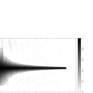
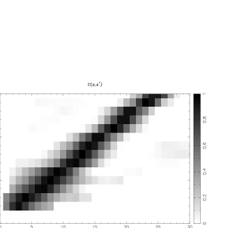
Figure 8: The measured ${\rm cor}(\rho^{s}(k,40),\rho^{s}(k,\eta))$ and the coherence function ${\cal C}_{\rho^{s}}(x,x^{\prime})$ it implies.

6.1 What can be measured from simulations

In Fig. 7 we plot the structure function of the strings’ energy density defined by $P(\rho^{s}(k,\eta))={F^{2}_{\rho^{s}}(x)/\eta}$, as discussed in [25]. There we show that this is well fitted with

$$F_{\rho^{s}}^{2}={N\over(1-2bx_{c}x+bx^{2})^{1/2}}$$ (61)

where $N$ is a constant, $b\approx.006$, and $x_{c}\approx 10$. Although we cannot measure the $x\ll 1$ region with the simulation it is known that a white noise behaviour is to be expected. Therefore we may safely take (61) as a valid extrapolation. The strings’ energy coherence function is plotted in Figure. 8. On the right we plot

$${\rm cor}(\rho^{s}(k,40),\rho^{s}(k,\eta))={{\langle\rho^{s}(k,40)\rho^{s}(k,\eta)\rangle}\over\sigma(\rho^{s}(k,40))\sigma(\rho^{s}(k,\eta))}$$ (62)

and on the left the ${\cal C}(x,x^{\prime})$ inferred from this measurement. The region $x<1,x^{\prime}<3$ has been left undetermined by the simulation, but since ${\cal C}(x,x^{\prime})$ is symmetric this leaves undetermined only $x<1,x^{\prime}<1$. We shall fill this gap with the widest range of possibilities. The last input required is $\Gamma$. In the Appendix we give some general properties imposed on equations of state by energy conservation.

Figure 9: The top three rows show a grid of cosmic strings’ spectra $P(\Theta_{0}+\Psi)$ for $\tau_{c}$ and $\chi_{c}$ varying within the allowed uncertainties. In dashed and dotted lines we have plotted a coherent and a totally incoherent approximation. The last row addresses the issue of how big the coherence time of a cosmic string would have to be for secondary oscillations with $\omega\approx 0.5$ to appear. The value $\tau_{c}=4$ is found, clearly ruled out by simulations.

Figure 10: The marginally acceptable (given simulations) cosmic string parameters which are most favourable for secondary oscillations: large coherence time $\theta_{c}=6$, coherent filling in the region where ${\cal C}(x,x^{\prime})$ could not be measured, low values of compensation scale $\chi_{c}$. On the right we show $l(l+1)C_{l}$ spectra from the monopole (dash) and dipole (point-dash) terms, in these cases. As for inflation the monopole dominates. Even pushing causality ($\chi_{c}=2$) one does not obtain meaningful oscillations. On the left we show the structure functions $x^{4}F(x)$ for the various $\chi_{c}$ parameters considered. Broad peaks centred around $x=10$ are always obtained.

6.2 The effects of the compensation and coherence time

We assume that stress-energy components other than $\rho^{s}$ can be ignored for the purpose of studying secondary oscillations (we take this question up further in the appendix). We therefore set $\Gamma=1$. The main uncertainty from the simulations concerns the strings coherence time. From Figs. 8 this can be estimated to be $\theta_{c}\approx 3-6$ (corresponding to $\tau_{c}\approx 1.5-2.5$). There is some evidence that $\tau_{c}$ decreases at large $x$. We shall fill in the region $x<1,x^{\prime}<1$ in three ways: same coherence function as in outer region; incoherent filling, in which one sets $\tau_{c}=0$ in this region; and coherent filling, in which one sets ${\cal C}=1$ in this region. These cases cover the extreme possibilities for the behaviour of ${\cal C}$ where it was not measured. Another uncertainty is the compensation scale $\chi_{c}$. This may be liberally placed in the region $2<\chi_{c}<5$. Within the framework of all that is already known this uncertainty has little impact.

The top three rows of Fig.9 show a grid of spectra in which $\tau_{c}$ and $\chi_{c}$ are varied within the allowed uncertainties. In dashed and dotted lines we have also plotted a coherent and a totally incoherent approximation (using $P$ rather than $P^{r}$). We have redone Fig.9 with coherent, incoherent, and trivial fillings in the $x<1,x^{\prime}<1$ region and found the results nearly identical. Clearly strings tend to erase secondary oscillations. For central values favoured by simulations this is done very effectively. For the marginally acceptable case where $\tau_{c}=2.5$, $\chi=2$ we cannot rule out the existence of very soft undulations in $P(\Theta_{0}+\Psi)$. The bottom row of Fig.9 addresses the issue of how big the coherence time of a cosmic string would have to be for secondary oscillations to show up. Even accepting $\omega=0.5$ as a reasonable oscillation strength, it appears that $\theta_{c}\approx 10$ is required. This is ruled out by simulations.

In order to argue that despite simulation uncertainties, we have established cosmic string’s absence of secondary oscillations, we now concentrate on the marginally acceptable scenario most favourable for secondary oscillations. We choose the extreme value $\tau_{c}=2.5$ and fill the unmeasured domain of ${\cal C}$ coherently. We then allow $\chi_{c}$ to take values $2,\cdots,5$. As we have seen the monopole power spectrum then shows an undulation. These are not even minima, but mere platforms in the rising spectrum. In Fig. 10 we show the $C_{l}$ spectrum they translate into. We have included Silk damping, combined the monopole with the dipole, and free streamed the result into $C_{l}$’s. Even in the most extreme case of compensation scale $\chi_{c}=2$ (pushing causality) the resulting $C_{l}$ undulations are extremely soft. Overall it is clear that the coherent approximation for cosmic strings will grossly overestimate the oscillatory structure of the spectrum. The totally incoherent approximation, on the other hand, simply exaggerates the lack of oscillations found in the real case.

This result may be understood by looking at the form of the potential source term $x^{4}F(x)$ in Fig. 10. This is dominated by the shape of $F_{\rho^{s}}(x)$. A low compensation scale may enhance the power on larger scales, and shift the peak in $x^{4}F(x)$ to the left. However one would need to push causality limits in order to distort the strings’ peak significantly. $\chi=2$ is the most that can be done realistically. In general $x^{4}F(x)$ for cosmic strings will have a very broad peak placed at $x=x_{c}\approx 10$. Hence each mode will be active for a long time, requiring a very large coherence time for effective coherence. The relatively low coherence time measured then suggests effective total incoherence, and since $x^{4}F(x)$ is broad, this will have time to erase the secondary oscillations. Also note that the double integral (41) is dominated by a region centred at $x=x^{\prime}\approx 10$. Hence it is in this region that knowledge of ${\cal C}(x,x^{\prime})$ is most relevant. This explains why our results are so insensitive to the way in which the unmeasured region $x<1,x^{\prime}<1$ is filled. Since we also expect that the low $x$ region is where corrections due to string loops and gravity waves are largest, the unimportance of this region gives us added confidence in our qualitative results.

6.3 The cosmic strings $C_{l}$ spectrum in the totally incoherent approximation

Figure 11: The $C^{l}$ spectrum for I (dash) and X (line) cosmic strings. The top lines use $s=.1,\sigma=.4$ for X strings and $s=.15,\sigma=.45$ for I strings. The bottom lines both use $s=.2,\sigma=.5$. We have assumed $\Omega=1$, $h=.5$, and $\Omega_{b}=0.05$.

Since the totally incoherent approximation seems to be justified for cosmic strings we have solved the full H+S algorithm in this approximation. We use the expression from [24] for the time-integrated power spectrum

$$P^{r}(\rho^{s})={1\over 1+2(\beta x)^{2}}$$ (63)

We consider the two cases $\beta=1$ and $\beta=.3$ similar to the X and I models in [24]. We consider only scalar contributions. We assume that the defect variables are subject to equations of state of the form $p^{s}=\gamma(x)\rho^{s}$, $\Pi^{s}=\eta^{2}\gamma_{s}(x)\rho^{s}$, and $v^{s}=\eta\gamma_{v}(x)\rho^{s}$. Energy conservation at small $x$ requires that $3\gamma(0)=(1/2\alpha)-1$ and $\gamma_{v}(0)=(1-2\alpha)/(3\alpha(4\alpha+1))$, with $\alpha=\eta h$ (see appendix). We make use of a string simulation to determine the large $x$ behaviour. We find, with large uncertainties, that $x\gamma_{v}(x)=s\approx.1-.3$, and $x^{2}\gamma^{s}(x)=\sigma\approx.4-.55$. We interpolate between the $x\gg 1$ and $x\ll 1$ behaviour. We set $\Pi=0$ and assume that $a^{2}\rho\Delta_{T}$ is subdominant except for the compensation and we fix the compensation scale at $\chi_{c}=2\pi$. Using (14) and (15) we finally obtain the required cosmic strings potential structure functions to be inserted in the HS formalism as modified for incoherent perturbations. The results are plotted in Fig. 11. The Sachs-Wolfe plateau exhibits a “running” tilt ranging from $n\approx 1.4$ before $l=10$ to $n\approx 1.2$ at $30-40$, although this is quite sensitive to input uncertainties. There is a single Doppler bump located at $l\approx 400-600$. These last two features are remarkably robust against uncertainties in the strings energy structure function, compensation and equations of state. The peak position is affected mostly by the energy structure function. The lower side of the $l\approx 400-600$ range appears to be favoured by X strings, and the upper side by I strings. The effect of equations of state on the peak position is negligible. An unnaturally strong compensation on small scales could push the peak further to the right but this is unlikely. The absence of secondary oscillation is a permanent feature whatever parameters changes one introduces, within the ranges mentioned above. The ratio between the peak and the plateau heights, on the other hand, can change by as much as an order of magnitude. Even small changes in the equations of state appear to be relevant. This is because the ISW plateau and the intrinsic terms probe different combinations of defect stress-energy components. One may hope that the peak/plateau height may act as a powerful probe of the defect speed and viscosity composition. On the other hand a prediction of the peak/plateau height ratio for strings will have to wait for improved simulations.

7 Conclusions

We have developed our formalism along two lines. We isolated the differences between inflation and defects which we found important for Doppler peak features. These were cast into the concepts of active and passive fluctuations, and coherent and incoherent fluctuations. These concepts allowed us to discuss Doppler peak features for a generic abstract defect, before addressing any concrete example. In order to address concrete examples we had to develop formalism along a second line. We extended the Hu and Sugiyama formalism so as to accommodate topological defect theories. The extensions concern mainly the way in which averages are taken when the photon fluid is being driven incoherently. We also allowed for photon backreaction effects so as to take into account the causality-required compensation.

We then derived two types of results. We studied Doppler peaks’ position and the structure of secondary oscillations for a generic defect, and then for cosmic string theories. We found that generic defects place the primary peak on or to the right of the adiabatic position ($l\approx 220$ for sCDM cosmological parameter values). The shift to the right, when present, is always additive, in contrast with low $\Omega$ models, which apply a multiplicative type of shift. The value of the shift is controlled by a single parameter $x_{c}$ which can be identified as $x_{c}\equiv 2\pi\eta/\xi_{c}$, where $\xi_{c}$ is roughly the coherence length of the defect. Very large defects, on the verge of violating causality, produce no shift. The smaller the defect coherence length, the larger its shift. The texture out-of-phase signature found by [11, 12] is therefore an accident related to the particular value of $x_{c}$ for textures, and not a generic defect feature.

We also found that the structure of secondary oscillations may be radically different for generic defects. This is generally controlled by the ratio of the defect scaling coherence time $\theta_{c}$ and $x_{c}$. If $\theta_{c}\gg x_{c}$ then the defect is effectively coherent, and displays secondary oscillations like the inflationary ones. If this is not the case then the secondary oscillations still appear if the defect structure function is sufficiently narrow, typically placing the primary peak close to the adiabatic position. Defects with a main peak shifted to the right, however, typically have broader structure functions. Provided that $\theta_{c}$ is not larger than $x_{c}$ the secondary oscillations get softer, the more so the further to the right the main peak is. Anywhere to the right of the isocurvature position, any defect with a realistic $\theta_{c}$ does not show secondary oscillations.

Given this picture there is good hope for a decisive experiment confronting inflation and defects. Defects and inflation can only be confused for $\Omega=1$ inflation, and a very large defect ($x_{c}\approx 2.7$). Only this annoying defect would leave no imprint of either its active or of its incoherent nature. Any other defect would leave some exotic imprint on the peak structure. An additive shift would ensure no confusion with low $\Omega$ inflation. Also the secondary peaks would normally appear as softer undulations for not too large $x_{c}$, or totally disappear for any realistic coherent times, if $x_{c}$ is large enough. No inflationary scenario could realize these spectra.

It remains to find out into which region of parameter space ($x_{c}$,$\theta_{c}$) each of the motivated defect scenarios fall. This is clearly a quantitative issue to be decided from simulations. We addressed this problem in connection with cosmic string theories. We measured the required structure and coherence functions. We found that even taking all the uncertainties into account cosmic strings fall into the class of defect theories for which the absence of secondary oscillations is a robust prediction. This validates the totally incoherent approximation, and we solved the H+S algorithm in this approximation for cosmic strings. The solution reveals that given the simulation uncertainties the main peak position should fall in $l\approx 400-600$. The height of the peak, however, is more sensitive to simulation uncertainties, and so we refrain from commenting on it at this stage.

Appendix: Active perturbations subject to equations of state

A complete solution for concrete defect models requires a precise knowledge of the defect stress energy power spectra. Knowledge of the stress energy of other related matter components (such as the loops and gravity waves into which the cosmic strings decay) is also essential[28]. Furthermore, the correlations between all these components must carefully taken into account. In the case of textures this problem is relatively simple because the textures and their primary decay producs are all excitations of the same scalar field which can be studied numerically. The cosmic string problem is much more complex, and further work is required before it is understood clearly. We present here the methodology used for this paper which may, with further study, provide a sound basis on which to address these questions. Our starting point is the concept of defect equations of state.

Coherent equations of state

Active perturbations may be subject to at most two independent coherent equations of state relating $\rho^{s}$, $p^{s}$, $v^{s}$, and $\Pi^{s}$. Let them be $p^{s}=\gamma(k\eta)\rho^{s}$, and $\Pi^{s}=\eta^{2}\gamma_{s}(k\eta)\rho^{s}$ for a scaling active perturbation. For a coherent perturbation the conservation equations will then impose another equation of state $v^{s}=\eta\gamma_{v}(k\eta)\rho^{s}$. The equations of state impart perfect equal-time correlation between all four variables (${\rm cov}(A,B)=\sigma(A)\sigma(B)$ for any two variables) and so (29) becomes the more general statement

$${\langle A({\bf k},\eta)B(-{\bf{k^{\prime}}},\eta^{\prime})\rangle}={\langle A(-{\bf{k}},\eta)B({\bf k^{\prime}},\eta^{\prime})\rangle}=\delta({\bf k}-{\bf k^{\prime}})\sigma(A(k,\eta))\sigma(B(k^{\prime},\eta^{\prime}))$$ (64)

where $\sigma(.)={\sqrt{P(.)}}$. This implies algebraic relations of the form $\langle\rho^{s}v^{s}\rangle=\sigma(\rho)\sigma(v^{s})$, $\langle{\dot{\rho}}\rho\rangle={\dot{\sigma}}(\rho)\sigma(\rho)$, or $\langle\dot{\rho}^{2}\rangle=({\dot{\sigma}}(\rho))^{2}$. Using them one can square the conservation equations (18) and (19), average, take the square root of the result, and find that the variances $\sigma(\rho^{s})$, etc, satisfy the same linear conservations equation as the variables $\rho^{s}$, etc, themselves. Introducing the variable $x=k\eta$, writing $\sigma(\rho^{s})=F_{\rho^{s}}(x)/\eta^{1/2}$ and $\sigma(v^{s})=F_{v^{s}}(x)\eta^{1/2}$ and denoting $d/dx$ by a prime one has:

$$xF^{\prime}_{\rho^{s}}+(\alpha(1+3\gamma)-1/2)F_{\rho^{s}}+x^{2}F_{v^{s}} = 0$$ (65)

$$xF^{\prime}_{v^{s}}+{\left(2\alpha+{1\over 2}\right)}F_{v^{s}}+{\left({2\over 3}x^{2}\gamma_{s}-\gamma\right)}F_{\rho^{s}} = 0$$ (66)

where $\alpha=\eta{\dot{a}}/a$. These can be solved expanding in Taylor series around $x=0$. Causality implies that $F_{\rho^{s}}(0)=const$, and isotropy implies that $\gamma_{s}(0)=const$. To zeroth order equations (65) and (66) imply that

$$3\gamma(0) = {1\over 2\alpha}-1$$ (67)

$$\gamma_{v}(0) = {1\over 3\alpha}{1-2\alpha\over 4\alpha+1}\;.$$ (68)

Fixing $\gamma_{s}(0)$ can also be done by extending the above calculation up to second order.

In this context the gauge-invariant formalism has the advantadge over synchronous gauge calculations that the potentials are also subject to equations of state of the form $\Phi=\eta^{2}\gamma_{\Phi}\rho^{s}$ and $\Psi=\eta^{2}\gamma_{\Psi}\rho^{s}$. This is because one may find a complete set of Einstein’s equations which are elliptic. One must bear in mind that the gauge invariant potentials may be expressed as combinations of synchronous gauge variables, and their time derivatives. Hence it is possible to get rid of potential time derivatives in Einstein’s equations, assuming source conservation, and write equations of state for the potentials. This advantage has one drawback: the defect structure function appearing as a potential source now combines the defect energy with its speed and viscosity, whereas in the synchronous gauge approach one only needs its pressure. Depending on the information available on the defect this may or may not be a problem. ¿From Einstein’s equations (14) and (15) we have

$$\gamma_{\Phi} = 4\pi\gamma_{c}{1+3\alpha\gamma_{v}\over x^{2}}$$ (69)

$$\gamma_{\Psi} = -4\pi{\left(\gamma_{c}{1+3\alpha\gamma_{v}\over x^{2}}+2\gamma_{s}\right)}\;.$$ (70)

These allow us to write the required relations

$$\sigma(\Phi G)= \eta^{3/2}\gamma_{int}F_{\rho^{s}}= \eta^{3/2}{\gamma_{\Phi}F_{\rho^{s}}\over(1+R)^{1/4}}{\left(1-(1+R){\gamma_{\Psi}\over\gamma_{\Phi}}+{3{\ddot{R}}\over 4k^{2}}-J^{2}\right)}$$ (71)

Using the conservation equations (18) and (19) we could also write $\dot{\Phi}$ and $\dot{\Psi}$ in terms of defect variables (and not their derivatives) and find a similar equation of state for the potentials appearing in the ISW term. The result is lengthy but straightforward to derive.

Small scale equations of state

On small scales the defects cannot be subject to coherent equations of state. For realistic sources it happens that $F_{\rho^{s}}(x)\propto x^{-n}$, and $\gamma$ and $k^{2}\Pi^{s}/\rho^{s}=x^{2}\gamma_{s}$ tend to a constant for $x\gg 1$. One may check that equations (65) and (66) would then lead to over-restrictive constraints (like $n=2\alpha-3/2$). We find from simulations that rather than relations like (64) on small scales one has

$${\rm cor}(A({\bf k},\eta),B(-{\bf k}^{\prime},\eta^{\prime}))\approx 0$$ (72)

where $A$ and $B$ are any two defect stress-energy components. This means that the different defect stress-energy components are in fact uncorrelated random variables, for which it makes more sense to postulate equations of state of the form:

$${\langle p^{s2}\rangle} = \gamma^{2}{\langle\rho^{s2}\rangle}$$

$${\langle v^{s2}\rangle} = \eta^{2}\gamma_{v}^{2}{\langle\rho^{s2}\rangle}$$

$${\langle\Pi^{s2}\rangle} = \eta^{4}\gamma_{s}^{2}{\langle\rho^{s2}\rangle}$$ (73)

We have found for cosmic strings that for large $x$

$$x\gamma_{v}(x) = s\approx.1-.3$$

$$x^{2}\gamma^{s}(x) = \sigma\approx.4-.55$$ (74)

The effect of the equations of state on cosmic strings coherence properties

¿From what we have said above the low $x$ behaviour of the $\Gamma$ factor (defined in (49)) is

$$\Gamma^{2}={\left(1+{1-2\alpha\over 1+4\alpha}+\gamma_{s}(0)\right)}^{2}$$ (75)

whereas its high $x$ behaviour is of the form

$$\Gamma^{2}=1+9\alpha^{2}{s^{2}\over x^{2}}+\sigma^{2}$$ (76)

In both regimes the $\Gamma$ factor is of order 1. Therefore $\Gamma$ may never modify the shape of the structure function $x^{4}F(x)$ as given by (49), which is determined by $F_{\rho^{s}}$ and the compensation factor. For this reason we simply set $\Gamma=1$ in our discussion of strings coherence features. On the other hand no doubt $\Gamma$ will affect the relative normalization of the structure functions used in the intrinsic and the ISW terms, which use different equations of state. We have found the the relative height of the peak and low $l$ plateau reflect sensitively the defect speed and viscosity composition.

Incoherent perturbations

If the perturbation is not coherent but is still subject to two equations of state, then all we have said still holds for the power spectra of the perturbation, but not for its time-integrated power spectra. One may try to relate power spectra and time-integrated power spectra. Suppose that one can factorize the unequal-time correlator as

$$P(\rho^{s}(k,\eta),\Delta\eta)=\sigma(\rho^{s}(k,\eta))\sigma(\rho^{s}(k,\eta+\Delta\eta)){\cal C}(k,\Delta\eta)$$ (77)

for, say, $\rho^{s}$. ${\cal C}(k,\Delta\eta)$ is a coherence function not necessarily symmetric about zero in $\Delta\eta$. Then wherever ${\cal C}\approx 1$ there is coherence, which is then cut off as ${\cal C}$ goes to zero for $\Delta\eta>\tau_{c}$. Suppose that this transition is very abrupt (e.g. ${\cal C}$ is nearly a step function). Then we can expand the time-integrated power spectrum written as in (33) in the form

$$P_{r}(\rho^{s}(k,\eta))=\tau_{c}^{(1)}P(\rho^{s}(k,\eta))+\tau_{c}^{(2)}\sigma(\rho^{s}(k,\eta)){\dot{\sigma}}(\rho^{s}(k,\eta))+{\tau_{c}^{(3)}\over 2}\sigma(\rho^{s}(k,\eta)){\ddot{\sigma}}(\rho^{s}(k,\eta))+{\cal O}(\tau_{c}^{4})$$ (78)

where

$$\tau_{c}^{(n)}={{\int}^{\infty}_{-\infty}}\,d\Delta\eta\;{\cal C}(k,\Delta\eta)(\Delta\eta)^{n-1}\;.$$ (79)

We have $\tau_{c}^{n}={\cal O}(\tau_{c}^{n})$. However, if ${\cal C}$ is symmetric about zero all the even $n$ vanish. We shall assume that this is not the case, so that the term in $\tau_{c}^{(2)}$ is the dominant correction to order ${\cal O}(\tau_{c}^{2})$. Using the conservation equations we can then write

$$P_{r}(\rho^{s}(k,\eta))=\tau_{c}P(\rho^{s}(k,\eta)){\left(1-{\hat{\tau}_{c}^{(2)}}(\alpha(1+3\gamma)+x^{2}\gamma_{v})\right)}$$ (80)

with ${\hat{\tau}_{c}^{(2)}}=\tau_{c}^{(2)}/(\tau_{c}\eta)$. For high $k$ the behaviour of $P$ and $P_{r}$ may be very different. For instance, for cosmic strings it is known that $P_{r}(\rho^{s}(k,\eta))\propto k^{-2}$ whereas $P(\rho^{s}(k,\eta))\propto k^{-1}$ ([24]). However for small $k$ equation (80) tells us that that $P_{r}$ and $P$ are related simply by a multiplicative constant. It can be checked that this is true for the power spectra of any variable. Moreover the multiplicative constant is the same ($\tau_{c}^{(1)}$) for all variables if one ignores corrections in ${\hat{\tau}_{c}^{(2)}}$. Therefore to this level of approximation the large scale behaviour of $P_{r}$ can be simply inferred from (67) and (68). If, however, one is to keep corrections of order ${\hat{\tau}_{c}^{(2)}}$ then the situation is more complicated, as the multiplicative constant depends on the variable. For a quantity related to $\rho^{s}$ by an equation of state of the form $\Gamma(k\eta)\rho^{s}$ one then has for $x\rightarrow 0$

$$P_{r}(\Gamma(k\eta)\rho^{s}(k,\eta))=\tau_{c}\Gamma^{2}(k\eta)P(\rho^{s}(k,\eta)){\left(1-{\hat{\tau}_{c}^{(2)}}(\alpha(1+3\gamma)+\Gamma^{\prime}/\Gamma)\right)}\;.$$ (81)

Higher derivatives of the $\gamma$’s at zero would be required to ${\cal O}({\hat{\tau}_{c}^{(2)}})$. How important these corrections are remains to be determined.

Modelling the $P_{r}$ on small scales is again more complicated and defect dependent. If the $\gamma$’s are always slowly varying one may use an approximation where formally $P_{r}=\eta\tau_{c}^{s}\sigma^{r2}$, where $\tau_{c}^{s}=\tau_{c}/\eta$, and $\sigma^{r}$ means the value of $\sigma$ as computed for coherent fluctuations but with $P(\rho^{s})$ replaced by $P_{r}(\rho^{s})$. Then the required potential properties can be found from

$$P_{r}(\Phi G) = \tau_{c}^{s}\eta^{4}\gamma_{int}^{2}F^{r2}_{\rho^{s}}$$ (82)

$$P_{r}({\dot{\Psi}}-{\dot{\Phi}}) = \tau_{c}^{s}\eta^{2}\gamma_{isw}^{2}F^{r2}_{\rho^{s}}$$ (83)

with $\gamma_{int}$ and $\gamma_{isw}$ are the equations of state for the potentials appearing in the intrinsic and ISW terms. We have used this approximation in the calculation in Section 6.3 of the $C_{l}$ spectrum of cosmic strings in the totally incoherent approximation.

References

- [1] M. White, D. Scott and J. Silk, Annu. Rev. Atron. Astrophys.32 319-370 (1994).
- [2] P. Steinhardt, Cosmology at the Crossroads to appear in the Proceedings of the Snowmass Workshop on Particle Astrophysics and Cosmology, E. Kolb and R.Peccei, eds. (1995) astro-ph/9502024.
- [3] T.W.B. Kibble, J. Phys., A9 1387-1398 (1976), A. Vilenkin and P. Shellard, Cosmic Strings and other Topological Defects. Cambridge University Press, Cambridge (1994). M. Hindmarsh and T.W.B. Kibble, Reports on Progress in Physics, 58, 477-562 (1995)
- [4] W.Hu and N.Sugyiama, Astroph.J., 444 489 (1995), W.Hu and N.Sugyiama, Phys. Rev. D, 51 2599-2630 (1995).
- [5] R. Battye, Small-angle anisotropies in the CMBR from active perturbations. IMPERIAL/TP/95-96/46
- [6] Bond J. R., Efstathiou G., MNRAS 226 655 (1987).
- [7] G. Jungman, M. Kamionkowski, A. Kosowsky and D. Spergel, Phys. Rev. Lett. 76 1007 (1996).
- [8] David Bennett, Albert Stebbins, and François Bouchet The Astrophysical Journal, Letters, 399, L5-8. (1992)
- [9] D. Bennett and S. Rhie, ApJ 406, L7 (1993).
- [10] D. Coulson, P. Ferreira, P. Graham and N. Turok, Nature 368 27-31 (1994).
- [11] R. Crittenden and N. Turok, Phys. Rev. Lett., 75 2642 (1995).
- [12] R. Durrer, A. Gangui and M. Sakellariadou, Phys. Rev. Lett., 76 579 (1996).
- [13] A. Albrecht, D. Coulson, P. Ferreira, and J. Magueijo, Phys. Rev. Lett. 76 1413-1416 (1996).
- [14] J.Traschen, Phys. Rev. D, 31 283-289 (1985); J.Traschen, Phys. Rev. D, 29 1563-1574 (1984).
- [15] J. Robinson and B. Wandelt, Phys.Rev.D 53 618 (1996).
- [16] N. Turok, Causality and the doppler peaks. astro-ph/9604172/
- [17] S. Veeraraghavan and A. Stebbins, Astrophys.J. 365 37-65 (1990).
- [18] U. Pen, D.N. Spergel and N. Turok, Phys. Rev. D, 49 692-729 (1994).
- [19] J.Magueijo, A. Albrecht, D. Coulson, P. Ferreira, Phys. Rev. Lett, 76 2617 (1996).
- [20] L.F.Abbott and J.Traschen, Astrophys.J. 302 39-42 (1986).
- [21] H.Kodama and M.Sasaki, Prog.Th.Phys. Supp., 78 1-166 (1984).
- [22] J.Magueijo, Phys. Rev. D, 46 3360-3371 (1992).
- [23] J.Magueijo et al, Causal compensated perturbations in the CMBR, in preparation.
- [24] A.Albrecht and A.Stebbins,Phys. Rev. Lett. 68 (1992) 2121-2124; ibid. 69 2615-2618 (1992).
- [25] P.Ferreira, A.Albrecht, D.Coulson, and J.Magueijo, in preparation.
- [26] Hu and White, Acoustic signatures in the cosmic microwave background, IASSNS-96/6.
- [27] J.Magueijo et al, Confusing defects and inflation, in preparation.
- [28] P. Avelino and R. Caldwell, Entropy perturbations due to cosmic strings astro-ph/9602116 (1996).