An approximate analytical method for inferring the law of gravity from the macroscopic dynamics: Thin-disk mass distribution with exponential density

Abstract

The gravitational potential and the gravitational rotation field generated by an thin-disk mass distribution with exponential density are considered in the case when the force between any two mass elements is not the usual Newtonian one, but some general central force. We use an approximation such that in the Newtonian case the gravitational field generated by the disk reduces to the familiar expression that results from applying the Gauss’ law. In this approximation, we invert the usual integral relations in such a way that the elemental interaction (between two point-like masses) is obtained as a function of the overall gravitational field (the one generated by the distribution). Thus, we have a direct way for testing whether it is possible or not to find a correction to the Newtonian law of gravity that can explain the observed dynamics in spiral galaxies without dark matter.

1 Introduction.

In a previous paper (Rodrigo-Blanco [1996] : hereafter, paper I ) we found the exact solution to the problem of, given the gravitational field generated by an spherical mass distribution with exponential density, finding out which was the elemental gravitational force, that is, the force between any two point-like masses, that could have generated that field.

In this paper we follow the same steps as in paper I , but the mass distribution that we consider is a thin disk with exponential density, which is a more realistic description of a spiral galaxy.

In this case, the exact solution cannot be found and the problem is solved in an approximation that, in the Newtonian case, is equivalent to use the Gauss’ law for calculating the gravitational field. We show that this is a very good approximation which improves even more when the $g_{\rm eff}(r)$, that represents the deviation from the Newtonian force, is a growing function of $r$, which is a welcome behaviour for explaining the observed data. We also see that this approximation is clearly better than using the results obtained in paper I for the case of spherical symmetry.

In Section 2 we give the general definitions that are used later in Section 3 for the case of a thin disk with exponential density. In Section 4 we show the mathematical basis underlying the results presented in Section 3. Finally we offer some conclusions. In Appendix A we study the validity of the approximation. In Appendix B we list some of the mathematical identities used in Section 4.

2 General definitions

Let us assume that the gravitational potential generated by a point-like mass does not correspond to the usual Newtonian form but can be written in terms of a function $g(r)$ that describes the deviation from the Newtonian law, that is,

$$\phi(r)\equiv-\frac{G_{0}m}{r}g(r).$$ (1)

The force per unit mass is, by definition, the gradient of the potential,

$$\vec{F}(r)\equiv-\frac{G_{0}m}{r^{2}}g_{\rm eff}(r)\frac{\vec{r}}{r},$$ (2)

where we have introduced

$$g_{\rm eff}(r)\equiv g(r)-rg^{\prime}(r).$$ (3)

In this way, to find the total potential or the total force generated by a mass distribution $\Omega$ with density $\rho(\vec{r})$, it is necessary integrate over the volume spanned by $\Omega$ to get:

$$\Phi(\vec{R})=-G_{0}\int\int\int_{\Omega}d^{3}\vec{r}\ \ \frac{g(|\vec{R}-\vec{r}|)}{|\vec{R}-\vec{r}|}\ \ \rho(\vec{r})$$ (4)

for the potential experienced by a point mass at a distance $R$ from the centre of $\Omega$, and

$$\vec{F}(\vec{R})=-G_{0}\int\int\int_{\Omega}d^{3}\vec{r}\ \ \frac{g_{\rm eff}(|\vec{R}-\vec{r}|)}{|\vec{R}-\vec{r}|^{2}}\ \ \frac{\vec{R}-\vec{r}}{|\vec{R}-\vec{r}|}\ \ \rho(\vec{r})$$ (5)

for the force.

In the case that the gravitational potential is only a function of the distance to the centre of the distribution, it is convenient to introduce two new functions $\Psi(R)$ and $\Psi_{\rm eff}(R)$ such that:

$$\Phi(R)\ \equiv\ -\ \frac{G_{0}M_{\rm tot}}{R}\ \Psi(R),$$ (6)

$$\vec{F}(R)\ \equiv\ -\frac{G_{0}M_{\rm tot}}{R^{2}},\ \Psi_{\rm eff}(R)\ \frac{\vec{R}}{R}$$ (7)

and the rotation velocity of a test particle in a circular orbit bound to the distribution will be:

$$V^{2}_{\rm rot}(R)\ \equiv\ \frac{G_{0}M_{\rm tot}}{R}\ \Psi_{\rm eff}(R)$$ (8)

where the auxiliary functions $\Psi_{\rm eff}(R)$ and $\Psi(R)$ satisfy the following relationship:

$$\Psi_{\rm eff}(R)=\Psi(R)-R\Psi^{\prime}(R),$$ (9)

Our goal is to design a procedure where, assuming that $\vec{F}(R)$ is known (say from observation of the rotation velocity) for all values of $R$, a $g_{\rm eff}(r)$ that generates the given rotation velocity is obtained. In other words, given the potential as inferred from observations we want to find which $g(r)$ could have generated it. Actually, we find $g(r)$ and $g_{\rm eff}(r)$ as functions of $\Psi_{\rm eff}(R)$ and $\Psi(R)$ respectively.

3 Thin-disk mass distribution with exponential density

The luminosity profile of many spiral galaxies can be well fitted assuming that the luminous matter is placed along a thin disk with a density that decreases exponentially with the distance to the centre of the galaxy (Kent [1987]).

$$\rho(r)\equiv\rho_{0}\ e^{-\alpha r}.$$ (10)

Considering a thin-disk distribution and using Eqs. (6), (7) and (10), in Eqs. (4) and (5), the two problems outlined above can be recast as two integral equations:

(i) Given $\Psi(R)$, defined by (6), find a function $g(r)$ such that:

$$\int_{0}^{\infty}dr\int_{0}^{\pi}d\theta\int_{0}^{2\pi}d\phi\frac{g(\sqrt{R^{2}+r^{2}-2Rr\cos\theta})}{\sqrt{R^{2}+r^{2}-2Rr\cos\theta}}r^{2}\sin\theta e^{-\alpha r}=\frac{8\pi}{\alpha^{3}}\frac{\Psi(R)}{R}.\\$$ (11)

(ii) Given $\Psi_{\rm eff}(R)$, defined by (7), find a function $g_{\rm eff}(r)$ such that:

$$\int_{0}^{\infty}dr\int_{0}^{\pi}d\theta\int_{0}^{2\pi}d\phi\frac{g_{\rm eff}(\sqrt{R^{2}+r^{2}-2Rr\cos\theta})}{(R^{2}+r^{2}-2Rr\cos\theta)^{\frac{3}{2}}}(R-r\cos\theta)r^{2}\sin\theta e^{-\alpha r}=\frac{8\pi}{\alpha^{3}}\frac{\Psi_{\rm eff}(R)}{R^{2}}.$$ (12)

In this case the problem cannot be solved exactly. We use an approximation that we call Gaussian as, in the Newtonian case, it is equivalent to use the Gauss’ law for calculating the gravitational field.

In the next section the calculations are described in detail. The solution to the two problems outlined above, in the Gaussian approximation can be summarized as:

(i) Potential problem: (viz. Eqs. (6) and (11))

In this case, the approximate solution to the problem is

$$g(x)=\Psi(x)-\frac{1}{\alpha^{2}}\Psi^{\prime\prime}(x),$$ (13)

where the function $\Psi$ has the following behaviour at the origin:

$$\Psi(0)\ =\ 0.$$ (14)

(ii) Force and velocity problem: (viz. Eqs. (7), (8) and (12)).

Here, the approximate solution is given by the following expression:

$$g_{\rm eff}(x)=\Psi_{\rm eff}(x)-\frac{1}{\alpha^{2}}\Psi_{\rm eff}^{\prime\prime}(x)+\frac{2}{\alpha^{2}x}\Psi_{\rm eff}^{\prime}(x)$$ (15)

and the behaviour of $\Psi$ at the origin is as follows:

$$\Psi_{\rm eff}(0)\ =\ \Psi_{\rm eff}^{\prime}(0)\ =\ 0.$$ (16)

4 Mathematical formalism.

First we show how to solve the potential problem, that is, how to go from equation (11) to equations (13) and (14). Then, the results obtained above are used to tackle the force problem, i.e, to go from equation (12) to equations (15) and (16).

4.1 The potential.

In order to go from equation Eq. (11) to Eqs. (13) and (14), it is necessary to use several mathematical identities. For convenience, these are listed in Appendix B.

Using (34), (36),(39) and (40) into (11) $\Psi(R)$ can be written as:

$$\begin{array}[]{rl}\Psi(R)=&-\frac{\alpha^{2}}{\pi\sqrt{R}}\sum_{\rm k=0}^{\infty}(4k+1)\left[\frac{\Gamma(2k+1/2)}{\Gamma(2k+1)}\right]^{2}\int_{0}^{\infty}dp\frac{\hat{g}_{s}(p)}{p}J_{\rm 2k+1/2}(pR)\int_{0}^{\infty}dre^{-\alpha r}\sqrt{r}J_{\rm 2k+1/2}(pr)\\ \end{array}$$ (17)

We apply our approximation here. We only consider the first term in the series of Bessel functions, that is, we drop all the terms in the series but the one with $k=0$. It can be seen, and we prove it in an appendix, that in the Newtonian limit (i.e, when $g(r)$ = $g_{\rm eff}(r)$ = $1$) this approximation corresponds to apply the Gauss’ law to the mass distribution, i.e, to say that the gravitational force at a distance $R$ is proportional to the total mass contained in the sphere of radius $R$. This is the reason why we have called this method Gaussian approximation. As it is quite a good approximation in the Newtonian case, and we also will see that it is exact for some forms of $g(r)$ and a very good approximation for the most interesting forms of $g(r)$, we restrict ourselves to consider only the first term in the series.

Thus, we will write:

$$\Psi_{0}(R)=-\frac{\alpha^{2}}{\sqrt{R}}\int_{0}^{\infty}dp\frac{\hat{g}_{s}(p)}{p}J_{\rm 1/2}(pR)\int_{0}^{\infty}dre^{-\alpha r}\sqrt{r}J_{\rm 1/2}(pr)$$ (18)

Now, using the functional form of $J_{\rm 1/2}$ and applying (35) to invert the Fourier transformation, and after some straightforward calculations, we get:

$$\Psi_{0}(R)=-\frac{\alpha}{2}\left\{e^{\alpha R}\left[\int_{0}^{R}dxg(x)e^{-\alpha x}-\int_{0}^{\infty}dxg(x)e^{-\alpha x}\right]-e^{-\alpha R}\left[\int_{0}^{R}dxg(x)e^{\alpha x}-\int_{0}^{\infty}dxg(x)e^{-\alpha x}\right]\right\}.$$ (19)

At this point, it is useful to introduce an auxiliary function $\psi(x)$ that makes the integrals exact:

$$g(x)\ \equiv\ \psi(x)-\frac{1}{\alpha^{2}}\psi^{\prime\prime}(x).$$ (20)

Eq (20) can be inserted into Eq. (19) and, upon integration by parts, we get:

$$\Psi_{0}(R)=\psi(R)-e^{-\alpha R}\psi(0),$$ (21)

where $\psi$ is a solution to the ordinary differential Eq. (20) that satisfies the conditions of being an analytic function at $x=0$, and

$$\lim_{x\rightarrow\infty}\psi(x)\exp(-\alpha x)=\lim_{x\rightarrow\infty}\psi^{\prime}(x)\exp(-\alpha x)=0.$$ (22)

These conditions are easily satisfied in all the astrophysical systems. The analiticity is satisfied in the Newtonian limit, which is the behaviour that we expect to recover at $R\sim 0$ and it can be seen that if Eq. (22) were not satisfied, the rotation velocity would grow almost exponentially with the distance, which clearly seems to contradict the observations.

It is straightforward to see that, provided $\psi(R)$ is a solution to Eq. (20), then $\Psi_{0}(R)$ is also a solution to the same equation. Moreover, the term proportional to $\psi(0)$ in Eq. (21) implies that $\Psi_{0}$ is zero at the origin. Taking all that into account, we finally obtain:

$$g(x)=\Psi(x)-\frac{1}{\alpha^{2}}\Psi^{\prime\prime}(x),$$ (23)

and

$$\Psi(0)\ =\ 0.$$ (24)

where we have omitted the subscript $0$ everywhere as we will in what follows.

4.2 The force and the rotation velocity.

Once $\Psi(R)$ is known, $\Psi_{\rm eff}(R)$ can be calculated using Eq. (9). Equivalently, once $g(r)$ is known, $g_{\rm eff}(r)$ can be obtained through Eq. (3). Using these two equations together with Eq. (23), and after some straightforward calculations, a direct relation between $g_{\rm eff}$ and $\Psi_{\rm eff}$ can be obtained:

$$g_{\rm eff}(x)=\Psi_{\rm eff}(x)-\frac{1}{\alpha^{2}}\Psi_{\rm eff}^{\prime\prime}(x)+\frac{2}{\alpha^{2}x}\Psi_{\rm eff}^{\prime}(x).$$ (25)

From Eq. (9) and the behaviour of $\Psi$ at the origin, Eq. (24), it is easy to see that, at the origin, $\Psi_{\rm eff}$ will satisfy:

$$\Psi_{\rm eff}(0)\ =\ \Psi^{\prime}_{\rm eff}(0)\ =\ 0.$$ (26)

5 Summary and conclusions.

We have found the solution to the problem of inverting the integral relation between the elemental law of gravity and the overall gravitational field generated by a thin-disk mass distribution. We have done it in an approximation that we have called Gaussian as it is equivalent to use the Gauss’ law for calculating the gravitational field generated by the distribution. Although this is not exact, we show in an appendix that it is a very good approximation, and it gets much better when $g_{\rm eff}(r)$ grows with $r$, which is the expected behaviour if the observed gravitational behaviour must be explained without the need of dark matter.

In summary, we now have a method for inferring $g_{\rm eff}(r)$ given $\Psi_{\rm eff}(R)$. It can be said that we have a way to travel from the world of macroscopic interactions to the world of microscopic interactions. It can be schematized as follows: Given the observed $V_{\rm rot}(R)$ for a given galaxy, use Eq. (8) to obtain $\Psi_{\rm eff}(R)$, fit it by a mathematical function and then use Eq. (15) to get the $g_{\rm eff}(r)$ that describes the elemental gravitational force (through Eq. (2)) that can explain the observed rotation curve.

We are now ready for applying the differential expression that we have found to the observed rotation curves of spiral galaxies, and find the $g_{\rm eff}$ required for explaining those rotation curves. Doing that, we will see whether it is possible or not to find a universal law of gravity that can explain all the rotation curves needing only the observed luminous matter. This will be done in a separate publication (Rodrigo-Blanco & Pérez-Mercader [1996]).

Appendix A The validity of the approximation.

In the step from Eq. (17) to Eq. (18) we made the approximation of considering only the first term of an infinite series. The terms dropped depend also on $g(r)$, which is not known, so it is not trivial to evaluate the goodness of the approximation.

In this appendix, we choose some functions $g_{\rm eff}(r)$ and compare the exact rotation velocity with the approximate one. By exact we mean the rotation velocity generated by the considered $g_{\rm eff}(r)$ through Eqs. (12) and (8). Nevertheless, for most functional forms of $g_{\rm eff}(r)$ an analytical solution cannot be found and it is necessary to perform numerical integration for finding that exact rotation velocity. Whenever that happens we have chosen to perform the integrals assuming that the disk has some non-zero thickness. Actually this is a more realistic model for a spiral galaxy, the astrophysical system to which our approximate method is applied. By approximate rotation velocity we mean the one such that the corresponding $\Psi_{\rm eff}(R)$ satisfies Eqs. (25) and (26).

As a test of consistency we first consider the Newtonian case, i.e., $g(r)=g_{\rm eff}(r)=1$. When we use Eqs. (25) and (26) we obtain:

$$\Psi_{\rm eff}(R)=1-(1+\alpha R)e^{-\alpha R},$$ (27)

and thus, the rotation velocity is

$$V^{2}_{\rm rot}(R)=\frac{G_{0}M_{\rm tot}}{R}[1-(1+\alpha R)e^{-\alpha R}]=\frac{G_{0}M(R)}{R},$$ (28)

where $M(R)$ is the disk mass inside the sphere of radius $R$. Of course, this is not the exact result, but it is what we find if we apply the Gauss’ law as an approximation for evaluating the gravitational field. That is why the approximation is called Gaussian.

Next, our approximation must be checked for other different forms of $g_{\rm eff}$. For doing that we choose a parametric family of $g_{\rm eff}(r)$’s given by

$$g_{\rm eff,\mu}(r)\equiv\left(\frac{r}{a}\right)^{\mu},$$ (29)

where $\mu$ parametrizes how fast $g_{\rm eff}$ grows.

Figure 1: Exact rotation curves (dots) and Gaussian approximation (solid line) when $g_{\rm eff}(r)\equiv\left(\frac{r}{a}\right)^{\mu}$ for some values of $\mu$ ($\mu=0$ is the Newtonian case). In every case, for the sake of clarity, the velocities are normalized by dividing by an appropriate constant ${\rm V}_{0}\equiv\frac{G_{0}M_{\rm tot}\alpha}{(\alpha a)^{\mu}}$. In the inset graphs (dashed lines) we have plotted, as a function of $r$ for each case, the percentage of error made when the Gaussian approximation is used instead of the numerical integrals.

Concerning the exact solution we have found the analytical one (for the thin-disk case) for $\mu=1$ and $\mu=3$:

$$V^{2}_{\rm rot,\mu=1}(R)=\frac{G_{0}M_{\rm tot}}{a}[1-(1+\alpha R)e^{-\alpha R}]=\frac{G_{0}M(R)}{R}\ \frac{R}{a},$$ (30)

$$V^{2}_{\rm rot,\mu=3}(R)=\frac{G_{0}M_{\rm tot}}{R}\ \left(\frac{R}{a}\right)^{3}\left(1+\frac{6}{\alpha^{2}R^{2}}\right).$$ (31)

For the other values of $\mu$ the integrals are performed numerically for a disk with a small thickness $h=\alpha^{-1}/6$

Concerning the approximation, it can be seen that, for $\mu=3$ the solution is (31), that is, the approximation is exact.

In Figure 1 we have plotted the exact rotation velocities compared with those corresponding to our approximation for some values of $\mu$. It can be seen that the results are very similar in every case. For each case, the solutions are normalized dividing by a convenient constant $V_{0}$ defined as:

$$V_{0}\equiv\frac{G_{0}M_{\rm tot}\alpha}{(\alpha a)^{\mu}}.$$ (32)

                                                                        

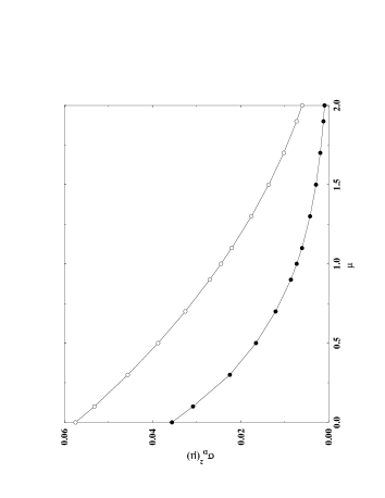
Figure 2: Mean square error in the velocity when the Gaussian approximation is used instead of the exact solution for the disk, as a function of $\mu$, and using $g_{\rm eff}(r)\equiv\left(\frac{r}{a}\right)^{\mu}$. The exact meaning of $\sigma^{2}_{\rm D}$ is explained in the text.

Although it can be seen in Figure 1 that the approximation is quite good in every case, and is better when $g_{\rm eff}(r)$ is a growing function of $r$, it is interesting to have a more quantitative way of describing the difference in the rotation velocity obtained in the exact case and in the Gaussian approximation as a function of $\mu$. In order to do that, we define a quantity $\sigma^{2}_{D}$ as follows:

$$\sigma^{2}_{D}(\mu)\equiv\frac{1}{N}\sum_{\rm i=1}^{N}\frac{(V_{\rm D,\mu}(r_{i})-V_{\rm G,\mu}(r_{i}))^{2}}{V^{2}_{\rm D,\mu}(r_{i})},$$ (33)

where the sub-scripts $D$ and $G$ stand for the disk (exact) and the Gaussian approximation, respectively. We sum over $r_{i}$, which are the points where the integrals are calculated. The total number of points for each value of $\mu$ is $N=100$.

So defined, $\sigma^{2}_{D}(\mu)$ is a measure of the mean square error that we make in the rotation velocity if the approximation is used instead of the numerical integrals, for each value of $\mu$.

In figure (2), we plot the value of $\sigma^{2}_{D}$ versus $\mu$. Once again, it can be seen that the larger $\mu$ is, the smaller the difference. We also plot the values of $\sigma^{2}_{D}$ obtained in paper I when the equations for spherical symmetry were used as an approximation to the disk problem. It can be seen that the Gaussian approximation is always better than the spherical one.

Appendix B Appendix: Mathematical identities

1. Fourier sine transform

   $$g(\sqrt{r^{2}+R^{2}-2rR\cos{\theta}})\equiv\frac{2}{\pi}\int_{0}^{\infty}\hat{g}_{s}(p)\sin(p\sqrt{r^{2}+R^{2}-2rR\cos{\theta}})dp$$ (34)

   $$\hat{g}_{s}(p)=\int_{0}^{\infty}g(t)\sin{pt}dt$$ (35)

2. Addition theorem for Bessel functions (see Gradshteyn [1980]).

   $$\frac{Z_{\nu}(m\omega)}{\omega^{\nu}}=\frac{2^{\nu}}{m^{\nu}}\Gamma(\nu)\sum_{\rm k=0}^{\infty}(\nu+k)\frac{J_{\rm\nu+k}(m\rho)}{\rho^{\nu}}\frac{J_{\rm\nu+k}(mr)}{r^{\nu}}C_{k}^{\nu}(\cos{\theta})$$ (36)

   where:

   $$\left\{\begin{array}[]{l}\omega\equiv\sqrt{r^{2}+\rho^{2}-2r\rho\cos{\theta}}\\ \rho<r\\ C_{k}^{\nu}\equiv\mbox{Gegenbauer Polynomials.}\end{array}\right.$$ (37)

   Using Eq. (36), together with:

   $$\sin(mz)=\sqrt{\frac{\pi mz}{2}}J_{\rm 1/2}(mz)$$ (38)

   we get:

   $$\frac{\sin{p\sqrt{r^{2}+R^{2}-2rR\cos{\theta}})}}{\sqrt{r^{2}+R^{2}-2rR\cos{\theta}}}=\frac{\pi}{2\sqrt{Rr}}\sum_{\rm k=0}^{\infty}(2k+1)J_{\rm k+\frac{1}{2}}(pr)J_{\rm k+\frac{1}{2}}(pR)P_{k}(\cos{\theta})$$ (39)

3. Legendre Polynomials.

   $$\int_{0}^{2\pi}d\theta P_{k}(\cos{\theta})=\left\{\begin{array}[]{lcl}2\left[\frac{\Gamma(2k+1/2)}{\Gamma(2k+1)}\right]^{2}&;&\mbox{if }k=2n+1\\ &&\\ 0&;&\mbox{if }k=2n\\ \end{array}\right.$$ (40)