The Las Campanas Redshift Survey

Abstract

The Las Campanas Redshift Survey (LCRS) consists of 26418 redshifts of galaxies selected from a CCD-based catalog obtained in the $R$ band. The survey covers over 700 square degrees in 6 strips, each 1.5$\arcdeg$ x 80$\arcdeg$, three each in the North and South galactic caps. The median redshift in the survey is about 30 000 km s^-1. Essential features of the galaxy selection and redshift measurement methods are described and tabulated here. These details are important for subsequent analysis of the LCRS data. Two dimensional representations of the redshift distributions reveal many repetitions of voids, on the scale of about 5000 km s^-1, sharply bounded by large walls of galaxies as seen in nearby surveys. Statistical investigations of the mean galaxy properties and of clustering on the large scale are reported elsewhere. These include studies of the luminosity function, power spectrum in two and three dimensions, correlation function, pairwise velocity distribution, identification of large scale structures, and a group catalog. The LCRS redshift catalog will be made available to interested investigators at an internet web site and in archival form as an Astrophysical Journal CD-ROM.

1 Introduction

Redshift surveys reveal surprising structures in the large-scale distribution of galaxies, which provide clues to physical properties of the Universe (see Giovanelli & Haynes (1991) and Strauss & Willick (1995) for reviews.) Early investigations (such as Kirshner et al. (1981), or Huchra et al. (1983)) suggested that the nearby Universe might be strongly inhomogeneous with nearly empty voids and thin, high contrast regions of galaxy overdensity. Convincing demonstrations that this pattern is a general feature of the Universe have come from extensive surveys which cover large angles on the sky, (de Lapparent et al. (1986), Geller & Huchra (1989):summarizing the CfA surveys, and da Costa et al. 1994a : the SSRS2 survey.) Galaxies appear to lie on networks of filaments or sheets extending over $100\ h^{-1}$ Mpc that encompass sharply bounded voids (Hubble constant $H_{0}=100\ h$ km s^-1 Mpc^-1). Despite the power of the CfA2 (Huchra et al. (1995)) and SSRS2 surveys in conveying an impression of the galaxy distribution on large scales, the largest features they reveal are very near the upper limit set by the depth of the survey at about 12000 km s^-1.

Are these the largest features in the Universe? There are hints of possible structure on larger scales from apparent periodicities in redshifts (Broadhurst et al. (1990)), from the flows suggested by Lauer & Postman (1994), or from possible variations in the luminosity density (da Costa et al. 1994a ). Only a deep extensive survey can provide evidence on the reality of these suggestions. Similarly, the statistical measures of galaxy clustering derived from redshift catalogs (Efstathiou (1995), Park et al. (1994)) which can be used to constrain models for the formation of structure in the Universe, have only modest precision at the large scales which are most interesting. To explore structure in the local Universe on a scale of 30000 km s^-1 and to improve our measures of galaxy statistics, we have been working since 1987 on the Las Campanas Redshift Survey (LCRS). We have compiled a CCD-based galaxy catalog, selected the galaxies, developed the fiber-optic equipment for mass producing galaxy spectra, and observed from 1988 to 1994. We have measured more than 26000 galaxy redshifts averaging $z=0.1$ over an area of 700 square degrees arranged in six long thin strips, three in the North Galactic Cap, and three in the South. The Las Campanas Redshift Survey provides a reconaissance of present-day structure on the largest scales mapped to date.

The Las Campanas Redshift Survey is a direct descendent of earlier surveys aimed at measuring the average properties of galaxies: the luminosity function and the space density of galaxies (Kirshner et al. (1978); Kirshner et al. (1979); Kirshner et al. (1983)) Annoying variations in the average properties, such as the luminosity density, signalled the presence of strong inhomogeneities in the galaxy distribution. Most startling was a large void of diameter $60\ h^{-1}$ Mpc in the galaxy distribution beyond the constellation Boötes (Kirshner et al. (1981); Kirshner et al. (1987); Kirshner et al. (1990)). Because similar structures are now frequently seen in wider-angle surveys and because the structures are nearly as large as the survey dimensions, a much larger and deeper survey seems needed in order to encompass a fair sample of the universe, as well as to search for structure on larger scales. The LCRS began with a goal of obtaining a galaxy sample of sufficient size, sky coverage, and depth to permit a reliable characterization of the average properties of galaxies and of their distribution.

While this work was in progress, some important large wide-angle redshift surveys have been carried out. Recent large-scale structure analyses include (see Strauss & Willick (1995) for a more complete list): (1) nearly all-sky samples of objects selected from the IRAS Point Source Catalog, specifically the IRAS 1.2 Jy survey (5321 galaxies with 60 $\mu$m flux $f_{60}>1.2$ Jy; Fisher et al. (1995)) and the 1-in-6 sparse-sampled IRAS QDOT survey (2184 galaxies with $f_{60}>0.6$ Jy; Lawrence et al. (1995)); (2) the Stromlo-APM survey, selected from the optical APM galaxy catalog, covering $4300$ square degrees of the Southern sky to a median survey depth $cz=15000$ km s^-1, but 1 in 20 sparse sampled (1787 galaxies, $b_{J}\leq 17.15$; Loveday et al. (1992); Loveday et al. (1995); Loveday (1996)); and (3) the combined CfA2 and Southern Sky (SSRS2) redshift surveys, selected from the Zwicky catalog and from plate scans, respectively, covering one-third of the sky over the North and South galactic caps out to a mean depth of about $7500$ km s^-1 (14383 galaxies with $m_{B(0)}\leq 15.5$; Huchra et al. (1995), da Costa et al. 1994a , 1994b). The CfA2+SSRS2 sample represents the state of the art for a wide-angle survey, with a large sample size and dense sky coverage. Sparse sampling provides an efficient way to measure a particular statistic, while dense sampling reveals structures that require the coherent arrangement of many galaxies and which are not easily characterized by low-order statistics. Our survey has some of the desirable properties of each: the samples are strips on the sky 1.5$\arcdeg$ wide and 80$\arcdeg$ long which are separated by 3$\arcdeg$. Within each strip, the galaxies are sampled randomly from a magnitude-limited catalog, but the sampling is quite dense, averaging about 70% of the magnitude-limited list. The distinctive properties of our survey are its depth (out to 60000 km s^-1) and the number of redshifts (26000).

The Las Campanas Redshift Survey provides improvements in sample size, volume, and depth in a limited region of the sky. Unlike most previously completed surveys, where spectra were taken of individual galaxies, one at a time, the LCRS employs a fiber-optic spectrograph system on the Las Campanas 2.5 meter DuPont telescope to observe over 100 objects at once. The greater depths explored by the LCRS mean that we observe galaxies which have sufficient surface density on the sky to make efficient use of a multi-fiber system. Some details of the galaxy selection and observing procedure which add to the complexity of the analysis were shaped by the properties of the fiber system, but the overall gain for exploring large-scale structure is very large. In this sense the LCRS represents part of a fundamental technological change in the way that large-scale redshift surveys are carried out.

Other surveys in progress, such as the Century Survey (Geller et al. (1996)) and the ESO-based survey (Vettolani et al. (1993)), have a comparable depth but cover smaller areas. Each has selection criteria that differ from ours in interesting ways which should make the comparison of our results with theirs a fruitful enterprise. The next generation of surveys, such as the 2 Degree Field project (Ellis (1993)) and the the Sloan Digital Sky Survey (Gunn & Weinberg (1995)), will use the multiplex advantage of fiber-fed spectrographs to obtain redshifts of up to a million galaxies, to about the same depth ($z\approx 0.1$) explored by the LCRS. It is our hope to illuminate some of the most interesting subjects for more thorough investigation by these ambitious projects.

In addition to providing a map of the galaxy distribution on the largest scales, the LCRS can help to constrain the physical history of the Universe and the properties of its constituents. Current theories of structure formation start with a spectrum of fluctuations produced in the early universe, follow the growth of structure due to gravitation, and strive to match both the subtle structure observed at recombination and the high-contrast distribution of the galaxies today mapped by redshift data. Most models presume that the Universe is dominated by non-baryonic dark matter (Blumenthal et al. (1984)) whose properties are to be inferred from the match to the data. The luminous galaxies trace the underlying mass, but may be biased: galaxies may form preferentially in peaks of the matter distribution (Bardeen et al. (1986), White et al. (1987)). Such models, with the aid of numerical N-body simulations, predict the clustering properties of galaxies from small nonlinear scales of less than $10\ h^{-1}$ Mpc, all the way up past the largest scales sampled by existing redshift surveys. The scales sampled with the LCRS, up to about $300\ h^{-1}$ Mpc, correspond to the horizon size at interesting stages in the early universe and are closer to the scales probed by microwave backgound observations than can be measured by smaller surveys. By observing galaxy fluctuations on these scales with LCRS, we can learn about primordial density fluctuations and the processes by which they grow. Combining evidence from large-scale structures and from microwave background observations holds the potential to answer fundamental questions about the dark matter that makes up most of the universe (Scott et al. (1995)).

This paper gives details about the construction of the LCRS which are essential to any analysis of the survey data. Some preliminary results and descriptions of the survey have already been published (Shectman et al. (1992), Oemler et al. (1993), Kirshner (1994), Lin 1995a , Shectman et al. (1995), Tucker et al. (1995).) Tucker’s (1994) Ph.D. thesis at Yale discusses the construction of the survey’s photometric catalog and statistical analyses of the early 50-fiber sample. Tucker describes the galaxy correlation function, the properties of galaxy groups, and galaxy clustering as a function of galaxy color. A more complete analysis, using the entire LCRS data set to investigate these topics, will be carried out by Tucker (Tucker et al. 1996c,a,b, respectively). Huan Lin’s Ph.D. thesis at Harvard (Lin 1995b ) is the basis for the present paper and for several forthcoming papers on the LCRS. Lin et al. (1996a) details the derivation of the luminosity function and space density of LCRS galaxies. Lin et al. (1996b) deals with the power spectrum, a basic statistic which characterizes the clustering properties of galaxies. Lin et al. (1996c) examines redshift-space distortions in the clustering of LCRS galaxies, derives the velocity dispersion of galaxy pairs, and estimates the value of the cosmological density parameter $\Omega$. The analysis of Landy et al. (1996) uses the tools of 2D Fourier analysis to search for coherent structures on very large scales in the LCRS data. Doroshkevich et al. (1996) examines the typical scales and types of large scale structure in the LCRS sample. Our intention is to make results from this survey and the survey data itself available to interested investigators. We have established a home page for the LCRS at “http://manaslu.astro.utoronto.ca/~lin/lcrs.html” which will provide rapid access to the data. An archival table of the redshift data will accompany this paper as an Astrophysical Journal CD-ROM.

2 Survey Construction

The Las Campanas Redshift Survey has been carried out at the Carnegie Institution’s Las Campanas Observatory in Chile, with redshifts harvested in a series of 13 spectroscopic observing runs from November 1988 through October 1994. Over 26000 galaxy spectra have been gathered, with an average redshift $z=0.1$, over 700 square degrees of the sky. This survey has exploited the Las Campanas 2.5-m DuPont telescope’s $2.1\arcdeg$-diameter field and the multiplexing capability of the associated multi-object fiber-optic spectrograph system constructed by Shectman, which permits simultaneous observations of 112 galaxy spectra.

The survey data may be divided into two parts based on the development of the photometric detectors and the fiber system during the six year span of the LCRS. The first 20% of the survey galaxies were selected based on data from an 800 x 800 TI CCD and the redshifts were measured using a 50-object fiber system. Beginning October 1991, an improved 112-object system was used to gather the final 80% of the data, which were also selected with better imaging systems using first a LORAL, then a large Tektronix CCD. See Table 1 for a summary. Some significant technical details of the survey construction, and additional specifics of the instruments and methods may be found in Shectman et al. (1992, 1995) and Tucker (1994), but essential features which affect the use of the sample for further analysis are set out here.

2.1 Photometry, Astrometry, and Object Selection

There was no suitable galaxy catalog available to us in 1986 when preparations for the Las Campanas survey began in earnest. We constructed our own catalog through a modest digital sky survey at the 1m Swope Telescope at Las Campanas. Photometry for the survey comes from CCD drift scans, taken through a Thuan-Gunn $r$ filter (Thuan & Gunn (1976)) with the telescope’s sidereal drive turned off. The accumulated charge is shifted across the chip at the sidereal rate and read out to produce a continuous strip of photometric data. Three CCD’s have been used in this way since the beginning of the survey. The first was a thinned 800 x 800 TI device, which was used with reimaging optics to obtain 1$\farcs$06 pixels. This was replaced in 1990 with a thick 2K x 2K LORAL chip, used without reimaging optics and binned 2 x 2 to provide 0$\farcs$865 pixels. The third CCD, introduced in 1992, is a thick 2K x 2K Tektronix CCD used unbinned without reimaging to provide 0$\farcs$692 pixels. Star-galaxy separation is appreciably better with the latter two chips because of the increased scale and the absence of distortion from intermediate optics.

The effective exposure time depends on the size of the chip and the cosine of the declination, but was typically near 1 minute. The limiting magnitude for the scans is similar to the limiting magnitude of the ESO red plates of the Southern Sky survey and extended well below the adopted limits near $m=17.75$ used for galaxy selection. Overlapping scans, offset in declination by slightly less than a chip width, were obtained to build up a strip $1.5\arcdeg$ wide. The typical length of each scan was $3\arcdeg$ or $4.5\arcdeg$ long: short enough to complete each $1.5\arcdeg$ x $3\arcdeg$ “brick” in about 2 hours, but long enough to minimize the time lost in setting the telescope and initiating the scan. Each brick covers two or three $1.5\arcdeg\times 1.5\arcdeg$ spectroscopic fields for the fiber system described below. A set of bricks was accumulated over several observing seasons to pave 700 square degrees, arranged in six long paths: in the North galactic hemisphere at $\delta=-3\arcdeg,-6\arcdeg,-12\arcdeg$ and in the South galactic hemisphere at $\delta=-39\arcdeg,-42\arcdeg$, and $-45\arcdeg$.

These drift scans were analyzed by an automated photometry system similar to that described in Kirshner et al. (1983). Bias was determined from an overscan region and subtracted from the data. The data were then sky-subtracted and flatfielded using the mode of the pixel values in each column and in each scan-line, respectively. Objects were found by a search routine which identified contiguous groups of pixels whose brightness was greater than 1.15 times that of the sky. Two magnitudes were derived for each object: an isophotal magnitude, $m$, corresponding to the sum of the background corrected flux in all pixels within the object, and a central magnitude, $m_{c}$, which measures the flux within a 2-pixel radius of the object center. The area measured by the central magnitude is close to that covered by a spectroscopic fiber and it is used to identify galaxies which have low central surface brightness. Images were classified using several structural parameters. All objects not classified as stars were inspected by eye to eliminate spurious galaxy classifications. Our star-galaxy separation criteria turned out to be conservative so that there is a small amount of stellar contamination in the spectroscopic sample (Table 1 and § 2.2). Figure 1 illustrates the stellar contamination rate as a function of isophotal magnitude and surface brightness.

Photometric calibration of the data proceeded in several steps. Observations were obtained only on nights which appeared to be photometric, and photometric standard fields were observed several times per night. These standards were used to obtain a zeropoint for each night’s scans. Though our photometry was obtained with a Gunn $r$ filter, the calibration was done relative to standards (Graham (1981); Graham (1982)) with magnitudes in the Kron-Cousins $R$ band, resulting in a hybrid red band which we call $R_{G;K-C}$. The zeropoint difference between $R_{G;K-C}$ and true Kron-Cousins $R$ is small ($<0.1$ mag), which can be seen in Figure 2 (see also Tucker (1994)).

This photometry calibrated the catalog from which objects were selected for spectroscopic observations. Even after the observations were obtained, we continued to refine the photometric calibration, so the resulting photometric limits for each brick vary slightly from the nominal values. Near the end of this survey, after scans were obtained of all bricks in each declination strip, additional calibration procedures were applied to eliminate residual photometric offsets. These offsets can be due to two effects. First, fluctuations in the derived zeropoints from night to night, and within some nights, reveal that not all of the nights on which data were obtained were perfectly photometric. Secondly, isophotal magnitudes of galaxies are quite sensitive to the limiting isophote. Because our outer isophote was defined as a multiple of the sky brightness, variations in sky brightness could cause variations in $m_{iso}-m_{total}$, as could variations in the seeing.

Because most of the bricks in a strip overlap their neighbors to the east and west, we could compare the photometric zeropoints of all the bricks within one, or at most a few, groups of contiguous bricks within each strip. This comparison, using the stars in the overlapping regions, revealed residual photometric offsets with a standard deviation of 0.065 mag. After removing these offsets, the zeropoint of each group of bricks was redetermined using CCD observations of 26 regions we obtained with Yale Service Observing Time on the CTIO 0.9 meter telescope, supplemented with objects from the HST photometric catalog. This comparison revealed no offsets in the mean of any group greater than $\sim 0.015$ mag.

To remove variations in $m_{iso}-m_{total}$, magnitudes were calculated for all objects through a 12 arcsec diameter synthetic aperture. This magnitude, $m_{12}$, is insensitive to seeing or sky brightness variations. Therefore, $m_{12}-m_{total}$, while a function of magnitude, should be constant from field to field. Intercomparison of $m_{iso}-m_{12}$ with $m_{iso}$ from field to field allows us to remove variations in $m_{iso}-m_{total}$ for galaxies. The field-to-field variation in this quantity had a standard deviation of 0.07 mag.

The final distribution of pairwise galaxy magnitude differences for galaxies which were measured twice on overlapping bricks is presented in Figure 3. This distribution has broader wings than expected from pure photon noise, but is otherwise as expected. From this distribution we calculate the standard deviation of galaxy magnitudes, $\sigma_{m}=0.10$, for $16.0<r\leq 17.0$, and $\sigma_{m}=0.17$ for $17.0<r\leq 18.0$.

The astrometric calibration of driftscan data is straightforward. To first order, the $x$ and $y$ coordinates within the data array map linearly into declination and right ascension, with two scale factors: telescope scale and CCD clock rate. Three additional correction factors may need to be applied: one for rotation of the CCD relative to the cardinal directions of celestial coordinates, a second for differential stellar aberration as the earth rotates during a scan, and, in the case of the early data taken with a focal reducer, a third for distortions in the optical system. Stellar aberration was calculated from first principles. Experience revealed that the other factors were all stable during a single observing run, and one global calibration of each was sufficient per run.

This calibration was done using the coordinate system defined by the HST Guide Star Catalog (Jenkner et al. (1990), Lasker et al. (1990), Russell et al. (1990)). The Guide Star Catalog has the virtue of containing a very dense sample, although individual positions are not very accurate (of order 1 arcsec) and it suffers from systematic errors of up to several arcsec near the edge of the individual Schmidt telescope fields from which the positions were derived. When averaged over all of the bricks observed in a single run, these errors are unimportant for determining the calibration parameters for the run. They are not, however, negligible for determining the coordinate zeropoints of each brick. When adjustment is made for systematic offsets between overlapping bricks, we find that the pairwise position differences between the bricks implies a standard deviation in the 1 dimensional position of an object $\sigma_{\alpha\delta}$ = 0$\farcs$25, for both stars and galaxies at all magnitudes in our catalog. However, because of the systematic zeropoint uncertainties, the absolute coordinates should not be trusted to better than 1 arcsec.

Two criteria are applied to select objects, classified as galaxies from the photometric catalog, for follow-up spectroscopy. First, both faint and bright isophotal magnitude limits are applied, with the following nominal values:

$$m_{1}\leq m<m_{2}:\left\{\begin{array}[]{ccc}m_{1}=16.0,&m_{2}=17.3,&{\rm 50\ fiber\ data}\\ m_{1}=15.0,&m_{2}=17.7,&{\rm 112\ fiber\ data}\end{array}\right.\ .$$ (1)

Second, the following nominal central surface brightness “cut line” is imposed:

$$m_{c}<m_{cen}-0.5(m_{2}-m):\left\{\begin{array}[]{ccc}m_{cen}=18.15,&{\rm 50\ fiber\ data}\\ m_{cen}=18.85,&{\rm 112\ fiber\ data}\end{array}\right.\ .$$ (2)

Figure 4 illustrates these selection criteria. Although they are more complex than a simple magnitude limit, they have their origin in the technique of our fiber optic measurements. Other surveys also have limits in surface brightness, but they are rarely made explicit: they result from failed observations. The faint isophotal limit $m_{2}$ is chosen so that there would generally be slightly more galaxies than fibers in each spectroscopic field. The bright isophotal limit $m_{1}$ is used so that the total count rate through the fibers, used to guide telescope pointing during the spectroscopic exposures, is not dominated by a few bright galaxies. The cut line limit on $m_{c}$ is used to eliminate low surface brightness (LSB) galaxies, for which it is difficult to obtain redshifts during the fixed exposure time of two hours. The slope of the line is chosen so that the fraction of LSB galaxies eliminated is approximately constant with isophotal magnitude, about 20% for the 50-fiber data, but $<10\%$ for the 112-fiber data (see Table 1).

When there are more objects that meet the photometric criteria than fibers available in a given 1.5$\arcdeg$ x 1.5$\arcdeg$ field, the targets for spectra were chosen at random from within the photometric boundaries. Careful use of this “galaxy sampling fraction” is required in subsequent analysis, but for the 112-fiber data that make up 80% of the sample, the galaxy selection fraction is large ($70\%$) and the details of this procedure do not affect the derived results for quantities like the luminosity density, once the sampling is taken into account. As described below, a small number of galaxy positions were physically impossible to observe because of fiber “collisions”, and their effects on the statistical measures also need to be assessed. In the unusual case where there were fewer galaxies than fibers for an individual field, the photometric limits were enlarged a small amount to admit additional targets until all the fibers were in use. However, for simplicity in the later data analyses, these additional galaxies, which constitute $<10\%$ of the total data set, are not considered part of the survey proper.

Table 2 details the right ascension and declination borders, photometric limits $m_{1}$, $m_{2}$, and $m_{cen}$, number of galaxy redshifts measured, and galaxy sampling fractions for each of the 327 spectroscopic fields of the Las Campanas survey proper. There are small variations in $m_{1}$, $m_{2}$, and $m_{cen}$ from the nominal values given above which result from recalibrations of the photometric zeropoints for the fields after the galaxies were selected and observed. Additional variations in $m_{cen}$ are caused by differences in pixel size of the 3 CCD’s used during the course of the survey, and by attempts to account for shifts in $m_{c}$ caused by variable seeing on the drift-scan images. Most photometry for galaxies observed with the 50-fiber system was obtained using our original 800 x 800 TI CCD, with 1$\farcs$06 pixels. The quality of the images was much improved for the larger chips used to obtain the 112-fiber data photometry and the analysis of the luminosity function (Lin et al. 1996a ) explicitly separates the 50-fiber data from the 112-fiber data to compute separate selection functions and luminosity functions for the two sets of data.

2.2 Spectroscopy and Redshift Measurements

A detailed description of the Las Campanas fiber system is given by Shectman (1993). The silica fibers have a 3$\farcs$5 diameter in the focal plane, are safely encased in concentric layers of hypodermic needle tubing and bicycle brake cable housing, and are manually plugged into holes on a 90-cm aluminum plate mounted at the curved focal plane of the Las Campanas 2.5-m DuPont telescope. The fibers guide the light from the objects into a spectrograph on the observing floor where the spectra are detected by the 2D-Frutti two-dimensional photon counter (Shectman (1984)). This combination consitutes the “fruit and fiber” system. Each plate is pre-drilled by a computer-controlled milling machine in Pasadena with holes at the expected positions of the selected objects. Holes for objects on four separate fields were drilled on a single plate, so that over 400 redshifts could be obtained during a single night using the 112-fiber system, without changing plates.

Mechanical constraints prevent the fibers from being plugged closer together than 55^′′. We have maintained a list of objects (about 1100) which were not observed because they were too close to another hole in the plate. In all other respects, these objects fulfill the selection criteria, including the random selection, and the list can be used to correct the small-scale correlation function and other statistics of the galaxy distribution. The galaxies which were not observed because of “collisions” are flagged in Table 3, the detailed listing of redshifts available on CD-ROM. Each field is one half of a photometric brick, with dimensions $1.5\arcdeg\times 1.5\arcdeg$, and the exposure times are typically 2 hours per field. Under 30 minutes are needed to change the observing setup from one exposure to the next, so a typical clear night produces four fields. For the 50-fiber system, there were an additional 10 fibers dedicated to observing sky spectra, and for the 112-fiber system, 16 sky fibers. Because the galaxies in the LCRS are equal to or brighter than the sky as observed through a fiber, precise sky subtraction was not required, and this sample of sky spectra proved adequate for our purposes.

The spectra are extracted, sky-subtracted, and wavelength-calibrated using a combination of custom programs and standard IRAF routines. For sky subtraction, all the sky spectra of a given exposure are averaged, then that average sky spectrum is normalized to the bright [OI] 5577 Å sky line of each raw object+sky spectrum, to account for individual fiber transmissions, before being subtracted. For wavelength calibration we use He-Ne arc lamp spectra taken with the fiber system midway through each object exposure. Some 35 lines in the range 3000-7000 Å are used to derive the wavelength solution. The typical rms wavelength residual for the comparison lines is 0.7 Å. The spectra are finally linearized and rebinned, at 2.5 Å per pixel (approximating the original pixel size), to the wavelength range 3350-6400 Å for the 50-fiber data or 3350-6750 Å for the 112-fiber data.

Redshifts are determined by cross-correlating the object spectra against a set of template spectra. The standard cross-correlation technique (Tonry & Davis (1979)) is implemented using the IRAF add-on package RVSAO (Kurtz et al. (1991), Mink & Wyatt (1995)). We use three templates, each consisting of an average of many high signal-to-noise stellar spectra. Two of the templates have strong absorption features typical of non-emission-line galaxies (see Sandage (1975)): CN (3833 Å), Ca H (3969 Å) and K (3934 Å), G-band (4304 Å), and Mg I (5175 Å). A third template contains strong Balmer absorption features: H$\beta$ (4861 Å), H$\gamma$ (4340 Å), and H$\delta$ (4102 Å). The third template is useful for obtaining cross-correlation velocities for the absorption-line features in galaxies with emission lines, for which such early-type Balmer absorption features are often seen. The third template avoids a systematic bias that creeps into cross-correlation velocities for the emission-line galaxies. This problem occurs for the first two templates because of systematic differences in the aborption-line spectra between the two templates and the typical galaxy with emission lines, particularly the increasing blend of H$\epsilon$ 3970 Å with Ca H. Gaussian profiles are fit to emission lines to determine redshifts from the line centers and also to measure line equivalent widths. The five most prominent emission lines present in our spectra are: [OII] 3727, [OIII] 5007, [OIII] 4959, H$\beta$ and H$\gamma$. The emission velocities from these lines are consistent to about 5 km s^-1, providing a check on our wavelength solutions, and the emission and third-template cross-correlation velocity zeropoints agree to 15 km s^-1. Two sample spectra, one with prominent absorption features and one with strong emission lines, are shown in Figure 5. One of the distinguishing features of the LCRS is that it has produced a very large and homogeneous set of galaxy spectra which are useful for characterizing the stellar populations and gas content of galaxies, not just their velocities (e.g., Zabludoff et al. (1996)).

Every spectrum is visually inspected at least once to check the plausibility of the automated cross-correlation and emission velocity determinations. Poor signal-to-noise spectra (approximately the bottom third) are examined more carefully and the final velocity determination, or rejection of the spectrum as a failure, is made interactively. We find that 93% of our spectra are galaxies, another 3% are stars contaminating our sample, and the final 4% fail to yield either a galaxy redshift or an identification as a star. Our rate for identifying spectra as galaxies or stars does not vary strongly with isophotal magnitude or central surface brightness; the identification rate only drops by about 5% at the faint isophotal magnitude limit or at the central surface brightness cut line (Lin et al. 1996a ). Our failure rate increases toward the edges of the DuPont telescope field (Shectman et al. 1995). This is a subtle effect whose impact on clustering statistics should be small, but which we are evaluating. Of the galaxy redshifts, 68% are cross-correlation velocities based on absorption lines alone, 25% are a combination of absorption and emission velocities, and the remaining 7% are solely emission velocities. A total of 26418 galaxy redshifts have been obtained in the course of the survey; 23697 of these galaxies lie within the photometric limits and geometric boundaries of the survey proper. The mean galaxy sampling fraction, corrected for stellar contamination, is 70% for the 112-fiber data and 58% for the 50-fiber data. Table 1 summarizes some of the above numbers for the main survey data samples. Because the spectroscopic fields are not observed more than once, the sampling fractions must be tracked on a field-by-field basis (as in Table 2) in subsequent statistical analyses of the survey data. Other surveys such as the Century Survey or the ESO Survey return to fields to observe every galaxy that meets their selection criterion, so it will be informative to compare results from these surveys with the LCRS to assess the effects of this choice. We expect they will be small (Lin et al. 1996b ; Tucker et al. 1996c ), but they are in the sense of the LCRS undersampling fields which have an unusually high density of galaxies, such as galaxy clusters.

The cross-correlation and emission-line fitting IRAF programs generate formal errors. We checked these estimates using a sample of 575 galaxies which were successfully observed twice, in the small overlapping areas between some of our spectroscopic fields. For our data, the formal errors underestimate the true random errors by 30%, so we multiply the formal errors by 1.3. Otherwise, application of a Kolmogorov-Smirnov (K-S) test (e.g. Press et al. (1992), § 14.3) shows that for these repeated galaxies, the shape of the cumulative distribution of velocity differences, normalized by the (corrected) velocity errors, is consistent with a gaussian distribution; see Figure 6(a). Figure 6(b) shows the distribution of corrected velocity errors for all galaxies and for the repeated galaxies; note that the two distributions are similar, suggesting that the result derived for the overlap sample applies equally well to the whole survey. The average random velocity error is 67 km s^-1, corresponding to $<1\ h^{-1}$ Mpc blurring in the spatial domain, so that none of the effects described by Schuecker, Ott and Seitter (1994) for low velocity precision redshifts is a problem for the LCRS. A measure of the zeropoint offset in the velocities is provided by the velocities of the stellar spectra, which should be near zero in the mean; we find $10\pm 1$ km s^-1 for the average of 1102 stars, not exactly zero but comfortably smaller than our random velocity errors.

3 The Survey Data

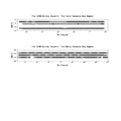
Figure 7: The survey pattern for the North (top) and the South Galactic Cap regions (bottom) sampled by the LCRS. Lightly shaded regions denote fields observed with the 50-fiber spectrograph and darkly shaded regions fields observed with the 112-fiber spectrograph. Declination and right ascension coordinates are epoch 1950.0.

The geometry of the survey is that of six “slices”, each about $1.5\arcdeg$ in declination by $80\arcdeg$ in right ascension. Three slices are located in the North galactic cap, centered at declinations $\delta=-3\arcdeg$, $-6\arcdeg$, and $-12\arcdeg$, and ranging in right ascension from $\alpha=10^{h}$ to $15.5^{h}$. The other three slices are in the South galactic cap, centered at declinations $\delta=-39\arcdeg$, $-42\arcdeg$, and $-45\arcdeg$, and ranging in right ascension from $\alpha=21^{h}$ to $4.5^{h}$. The fields are at galactic latitudes $b>30\arcdeg$ in the North and $b<-40\arcdeg$ in the South. Figure 7 shows the pattern of survey fields in declination and right ascension on the sky, with different shadings for 50- and 112-fiber fields. (Note that three fields in the $-45\arcdeg$ slice were not finished, thus producing gaps in the that slice. There are also other small gaps between fields that cannot be seen from the figures, so that one should always consult Table 2 for the exact boundaries.) The distributions of LCRS galaxies in redshift space, as a function of heliocentric velocity and right ascension, as well as their distributions on the sky, are next shown in Figures 8 (a-f) for each of the six slices, and in Figures 8 (g,h) for the combined Northern and Southern samples. For the $\delta=-3\arcdeg$ slice and the three Southern slices, the data combines 50-fiber and 112-fiber observations. The factor of two difference in sampling can be seen in the lower density of points for the 50-fiber fields in the figures. The $\delta=-6\arcdeg$ slice is nearly all 50-fiber data, and the $\delta=-12\arcdeg$ slice consists only of 112-fiber fields.

The figures demonstrate the rich texture of clusters, filaments, voids, and walls in the LCRS galaxy distribution, reminiscent of structures seen in the denser, wider, and shallower CfA survey (which has a mean distance of about 7500 km s^-1), but replicated many times across the bigger LCRS volume. The largest walls and voids have sizes of order $50-100\ h^{-1}$ Mpc, much smaller than the largest survey dimensions, suggesting that the LCRS samples the largest high-contrast structures of the nearby universe. The 3$\arcdeg$ separation between slices amounts to about $15\ h^{-1}$ Mpc at a typical survey redshift of 30000 km s^-1. The strong resemblance of one strip to its neighbor and the structures that are visible in the combined North or South fields provide another indication that coherent structures on scales of tens of Mpc are very common. The redshift data are found in Table 3, which is available in the AAS CD-ROM series.

Finally, redshift histograms for the 50- and 112-fiber North and South data sets are shown in Figures 16 and 17 along with the expected redshift distributions computed for galaxies uniformly distributed in space and sampled using the survey’s selection function as derived by Lin et al. (1996a). The average distance of the observed distribution is about $cz=30000$ km s^-1 as intended. Also, although large-scale structure makes the histogram noisy, the uniform distribution line is a reasonable approximation to the actual redshift distribution, which supports the view that the LCRS is large enough to approximate a fair sample of the nearby Universe.

We welcome other investigators to apply their analysis techniques to this large sample of galaxy redshifts. For this reason, the redshift catalog will be available at the LCRS home page (“http://manaslu.astro.utoronto.ca/~lin/lcrs.html”) and in the AAS CD-ROM series. To obtain reliable scientific results from this redshift data, users need to be aware of the details of our selection methods described and tabulated in this paper. These include the limits on isophotal magnitude and on central surface brightness, the differences between data taken with the 50 fiber system and with the 112 fiber system, and the limit on closest approach of the fibers. For many purposes, these effects can be taken into account quite easily, but the best use of the survey requires attention to these details.

Table 1: LCRS Sample Information

Sample	$N_{sel}$	$N_{lsb}$	%	$N_{gal}$	%	$N_{star}$	%	$N_{?}$	%	$f$
North 50	4288	1179	22	2711	92.2	130	4.4	99	3.4	0.66
South 50	4363	1145	21	2055	91.1	126	5.6	74	3.3	0.50
All 50	8651	2324	21	4766	91.7	256	4.9	173	3.3	0.58
North 112	12220	557	4	8552	94.9	153	1.7	302	3.4	0.71
South 112	15639	1530	9	10379	91.4	451	4.0	525	4.6	0.69
All 112	27859	2087	7	18931	93.0	604	3.0	827	4.1	0.70

Table 2: LCRS Spectroscopic Fields

Field	$\alpha_{1}$	$\alpha_{2}$	$\delta_{1}$	$\delta_{2}$	$m_{1}$	$m_{2}$	$m_{cen}$	$N_{fib}$	$N_{gal}$	$f$
1003-03W	10 03 30.60	10 09 46.42	-03 42 28.1	-02 16 03.4	15.06	17.76	19.41	112	111	0.87
1003-03E	10 09 46.42	10 16 05.81	-03 42 28.1	-02 16 03.4	15.06	17.76	19.41	112	109	0.75
1015-03W	10 16 05.81	10 21 46.37	-03 44 11.8	-02 15 11.2	14.86	17.56	18.71	112	93	0.56
1015-03E	10 21 46.37	10 28 00.72	-03 44 11.8	-02 15 11.2	14.86	17.56	18.71	112	109	0.57
1027-03W	10 28 00.72	10 33 26.78	-03 44 10.7	-02 15 22.0	16.01	17.31	18.31	50	42	0.58
1027-03E	10 33 26.78	10 39 33.77	-03 44 10.7	-02 15 22.0	14.91	17.61	18.76	112	106	0.65
1039-03W	10 39 33.77	10 45 30.41	-03 44 16.8	-02 15 14.4	14.94	17.64	18.79	112	97	0.67
1039-03E	10 45 30.41	10 52 00.53	-03 44 16.8	-02 15 14.4	14.94	17.64	18.79	112	101	0.79
1051-03W	10 52 00.53	10 57 34.87	-03 44 11.8	-02 15 09.4	16.09	17.39	18.29	50	32	0.89
1051-03E	10 57 34.87	11 03 00.26	-03 44 11.8	-02 15 09.4	16.09	17.39	18.29	50	33	0.94
1103-03W	11 03 00.26	11 09 30.94	-03 43 53.0	-02 14 52.4	14.94	17.64	18.79	112	105	0.55
1103-03E	11 09 30.94	11 16 00.74	-03 43 53.0	-02 14 52.4	14.94	17.64	18.79	112	109	0.54
1115-03W	11 16 00.74	11 21 29.57	-03 44 03.5	-02 15 02.2	14.73	17.53	18.63	112	95	0.83
1115-03E	11 21 29.57	11 27 00.17	-03 44 03.5	-02 15 02.2	14.73	17.53	18.63	112	67	0.85
1127-03W	11 27 00.17	11 33 28.37	-03 44 10.7	-02 14 55.7	14.88	17.58	18.73	112	109	0.71
1127-03E	11 33 28.37	11 39 58.06	-03 44 10.7	-02 14 55.7	14.88	17.58	18.73	112	105	0.52
1139-03W	11 39 58.06	11 45 26.45	-03 44 10.3	-02 15 05.8	14.81	17.61	18.71	112	97	0.57
1139-03E	11 45 26.45	11 51 31.18	-03 44 10.3	-02 15 05.8	14.81	17.61	18.71	112	110	0.43
1151-03W	11 51 31.18	11 57 30.24	-03 44 33.7	-02 15 08.6	15.01	17.71	18.86	112	88	0.86
1151-03E	11 57 30.24	12 03 42.31	-03 44 33.7	-02 15 08.6	15.01	17.71	18.86	112	95	0.90
1203-03W	12 03 42.31	12 09 31.32	-03 44 41.3	-02 15 16.2	15.05	17.65	18.85	112	96	0.89
1203-03E	12 09 31.32	12 15 31.30	-03 44 41.3	-02 15 16.2	15.05	17.65	18.85	112	108	0.59
1215-03W	12 15 31.30	12 21 28.97	-03 44 12.5	-02 15 09.7	14.79	17.59	18.69	112	104	0.86
1215-03E	12 21 28.97	12 27 29.74	-03 44 12.5	-02 15 09.7	14.79	17.59	18.69	112	104	0.89
1227-03W	12 27 29.74	12 33 27.70	-03 46 05.2	-02 15 20.9	15.92	17.22	18.07	50	33	0.82
1227-03E	12 33 27.70	12 39 18.65	-03 46 05.2	-02 15 20.9	15.92	17.22	18.07	50	48	0.91
1239-03W	12 39 28.66	12 45 27.94	-03 43 28.9	-02 15 25.9	15.85	17.15	18.00	50	25	0.45
1239-03E	12 45 27.94	12 51 19.46	-03 43 28.9	-02 15 25.9	15.85	17.15	18.00	50	43	0.76
1251-03W	12 51 23.11	12 57 21.41	-03 46 22.4	-02 15 34.9	15.83	17.13	18.08	50	47	0.63
1251-03E	12 57 21.41	13 03 13.54	-03 46 22.4	-02 15 34.9	15.83	17.13	18.08	50	47	0.37
1303-03W	13 03 30.26	13 09 25.20	-03 46 21.0	-02 15 19.4	16.00	17.30	18.15	50	45	0.68
1303-03E	13 09 25.20	13 15 19.58	-03 46 21.0	-02 15 19.4	16.00	17.30	18.15	50	39	0.89
1315-03W	13 15 26.62	13 21 20.71	-03 45 55.1	-02 15 04.3	15.88	17.18	18.13	50	49	0.67
1315-03E	13 21 20.71	13 27 13.63	-03 45 55.1	-02 15 04.3	15.88	17.18	18.13	50	50	0.53
1327-03W	13 27 28.51	13 33 24.96	-03 44 44.2	-02 15 39.2	16.03	17.33	18.33	50	50	0.59
1327-03E	13 33 24.96	13 39 29.93	-03 44 44.2	-02 15 39.2	14.93	17.63	18.78	112	107	0.81
1339-03W	13 39 30.62	13 45 30.00	-03 44 20.4	-02 15 33.8	14.81	17.61	18.71	112	78	0.72
1339-03E	13 45 30.00	13 50 59.86	-03 44 20.4	-02 15 33.8	14.81	17.61	18.71	112	80	0.89
1351-03W	13 50 59.86	13 57 31.73	-03 44 24.7	-02 15 29.9	14.77	17.47	18.62	112	104	0.93
1351-03E	13 57 31.73	14 04 00.00	-03 44 24.7	-02 15 29.9	14.77	17.47	18.62	112	96	0.86
1403-03W	14 04 00.00	14 09 30.10	-03 44 11.4	-02 15 21.2	14.78	17.58	18.68	112	94	0.85
1403-03E	14 09 30.10	14 14 59.52	-03 44 11.4	-02 15 21.2	14.78	17.58	18.68	112	89	0.92
1415-03W	14 14 59.52	14 21 24.12	-03 44 21.1	-02 15 18.7	15.01	17.71	18.86	112	103	0.91
1415-03E	14 21 24.12	14 27 57.67	-03 44 21.1	-02 15 18.7	15.01	17.71	18.86	112	108	0.91
1427-03W	14 27 57.67	14 33 31.15	-03 44 47.8	-02 15 49.3	16.14	17.44	18.44	50	26	0.83
1427-03E	14 33 31.15	14 39 00.34	-03 44 47.8	-02 15 49.3	16.14	17.44	18.44	50	41	0.88
1439-03W	14 39 00.34	14 45 25.46	-03 44 17.5	-02 15 14.0	15.11	17.81	18.96	112	107	0.72
1439-03E	14 45 25.46	14 51 57.19	-03 44 17.5	-02 15 14.0	15.11	17.81	18.96	112	108	0.91
1451-03W	14 51 57.19	14 57 11.54	-03 46 22.8	-02 15 37.1	15.96	17.26	18.11	50	37	0.70
1451-03E	14 57 11.54	15 03 02.04	-03 46 22.8	-02 15 37.1	15.96	17.26	18.11	50	25	0.97
1503-03W	15 03 02.04	15 09 30.22	-03 44 12.1	-02 15 14.0	14.76	17.56	18.66	112	63	0.92
1503-03E	15 09 30.22	15 15 30.17	-03 44 12.1	-02 15 14.0	14.76	17.56	18.66	112	100	0.72
1515-03W	15 15 30.17	15 21 30.82	-03 44 38.0	-02 15 43.6	14.89	17.69	18.79	112	66	0.91
1515-03E	15 21 30.82	15 27 30.02	-03 44 38.0	-02 15 43.6	14.89	17.69	18.74	112	62	0.91
1003-06W	10 03 30.96	10 09 52.32	-06 42 12.6	-05 15 49.0	15.00	17.70	19.35	112	100	0.55
1003-06E	10 09 52.32	10 16 08.62	-06 42 12.6	-05 15 49.0	15.00	17.70	19.35	112	92	0.88
1015-06W	10 16 08.62	10 21 17.71	-06 43 56.3	-05 15 33.8	15.98	17.28	18.13	50	38	0.39
1015-06E	10 21 17.71	10 27 06.96	-06 43 56.3	-05 15 33.8	15.98	17.28	18.13	50	44	0.81
1027-06W	10 27 30.82	10 33 33.17	-06 44 26.9	-05 15 13.3	15.92	17.22	18.22	50	45	0.66
1027-06E	10 33 33.17	10 39 37.18	-06 44 26.9	-05 15 13.3	15.92	17.22	18.22	50	38	0.76
1039-06W	10 39 37.18	10 45 02.45	-06 43 53.4	-05 15 25.2	16.26	17.56	18.41	50	44	0.90
1039-06E	10 45 02.45	10 51 06.14	-06 43 53.4	-05 15 25.2	16.26	17.56	18.41	50	46	0.48
1051-06W	10 51 31.66	10 57 11.11	-06 44 15.0	-05 15 23.0	16.08	17.38	18.28	50	48	0.60
1051-06E	10 57 11.11	11 03 27.31	-06 44 15.0	-05 15 23.0	16.08	17.38	18.28	50	48	0.66
1103-06W	11 03 28.44	11 09 18.22	-06 44 19.0	-05 15 27.4	16.03	17.33	18.28	50	40	0.93
1103-06E	11 09 18.22	11 15 05.64	-06 44 19.0	-05 15 27.4	16.03	17.33	18.28	50	39	0.51
1115-06W	11 15 30.91	11 21 28.03	-06 44 31.6	-05 15 26.3	16.08	17.38	18.38	50	48	0.83
1115-06E	11 21 28.03	11 27 38.09	-06 44 31.6	-05 15 26.3	16.08	17.38	18.38	50	50	0.85
1127-06W	11 27 38.09	11 33 11.81	-06 31 41.2	-05 15 32.0	16.01	17.31	18.16	50	48	0.69
1127-06E	11 33 11.81	11 39 05.69	-06 31 41.2	-05 15 32.0	16.01	17.31	18.16	50	36	0.93
1139-06W	11 39 28.82	11 45 30.91	-06 44 22.9	-05 15 01.1	14.98	17.68	18.83	112	109	0.74
1139-06E	11 45 30.91	11 51 34.61	-06 44 22.9	-05 15 01.1	16.08	17.38	18.38	50	47	0.52
1151-06W	11 51 34.61	11 57 09.77	-06 44 21.1	-05 15 27.0	16.04	17.34	18.19	50	45	0.65
1151-06E	11 57 09.77	12 03 07.08	-06 44 21.1	-05 15 27.0	16.04	17.34	18.19	50	46	0.58
1203-06W	12 03 30.98	12 09 36.02	-06 44 44.9	-05 15 18.7	16.02	17.32	18.22	50	46	0.63
1203-06E	12 09 36.02	12 15 36.74	-06 44 44.9	-05 15 18.7	16.02	17.32	18.22	50	46	0.42
1215-06W	12 15 36.74	12 21 16.92	-06 44 15.7	-05 15 38.9	16.07	17.37	18.22	50	41	0.92
1215-06E	12 21 16.92	12 27 07.68	-06 44 15.7	-05 15 38.9	16.07	17.37	18.22	50	37	0.93
1227-06W	12 27 30.17	12 33 27.58	-06 44 22.9	-05 15 23.8	16.16	17.46	18.36	50	38	0.76
1227-06E	12 33 27.58	12 39 36.74	-06 44 22.9	-05 15 23.8	16.16	17.46	18.36	50	48	0.68
1239-06W	12 39 36.74	12 45 11.78	-06 44 15.4	-05 15 28.4	16.13	17.43	18.28	50	43	0.47
1239-06E	12 45 11.78	12 51 06.84	-06 44 15.4	-05 15 28.4	16.13	17.43	18.28	50	43	0.47
1251-06W	12 51 29.11	12 57 28.78	-06 44 39.1	-05 15 12.2	16.10	17.40	18.40	50	46	0.76
1251-06E	12 57 28.78	13 03 33.10	-06 44 39.1	-05 15 12.2	16.10	17.40	18.40	50	47	0.53
1303-06W	13 03 33.10	13 09 22.85	-06 44 19.0	-05 15 36.7	16.28	17.58	18.43	50	44	0.51
1303-06E	13 09 22.85	13 15 05.14	-06 44 19.0	-05 15 36.7	16.28	17.58	18.43	50	39	0.51
1315-06W	13 15 28.56	13 21 38.35	-06 44 37.7	-05 15 29.5	15.00	17.70	18.85	112	68	0.71
1315-06E	13 21 38.35	13 27 29.02	-06 44 37.7	-05 15 29.5	16.10	17.40	18.30	50	28	0.84
1327-06W	13 27 29.02	13 33 17.66	-06 44 25.4	-05 15 50.4	15.98	17.28	18.13	50	50	0.93
1327-06E	13 33 17.66	13 39 07.70	-06 44 25.4	-05 15 50.4	15.98	17.28	18.13	50	48	0.59
1339-06W	13 39 31.06	13 45 34.39	-06 31 58.4	-05 15 06.1	16.03	17.33	18.23	50	47	0.70
1339-06E	13 45 34.39	13 51 35.93	-06 31 58.4	-05 15 06.1	16.03	17.33	18.23	50	40	0.89
1351-06W	13 51 35.93	13 57 15.53	-06 44 16.8	-05 15 37.4	15.83	17.13	17.98	50	31	0.92
1351-06E	13 57 15.53	14 03 04.18	-06 44 16.8	-05 15 37.4	15.83	17.13	17.98	50	49	0.72
1403-06W	14 03 31.75	14 09 34.92	-06 44 52.4	-05 15 46.8	16.07	17.37	18.37	50	43	0.64
1403-06E	14 09 34.92	14 15 36.55	-06 44 52.4	-05 15 46.8	16.07	17.37	18.37	50	48	0.83
1415-06W	14 15 36.55	14 21 07.15	-06 19 08.8	-05 15 51.5	16.06	17.36	18.21	50	36	0.82
1415-06E	14 21 07.15	14 27 06.41	-06 19 08.8	-05 15 51.5	16.06	17.36	18.21	50	17	0.86
1427-06W	14 27 28.70	14 33 45.29	-06 44 51.4	-05 40 55.2	16.10	17.40	18.30	50	26	0.86
1427-06E	14 33 45.29	14 39 35.18	-06 44 51.4	-05 40 55.2	16.10	17.40	18.30	50	26	0.76
1439-06W	14 39 35.18	14 45 18.74	-06 44 25.8	-05 15 51.1	16.18	17.48	18.33	50	45	0.66
1439-06E	14 45 18.74	14 51 06.48	-06 44 25.8	-05 15 51.1	16.18	17.48	18.33	50	42	0.62
1451-06W	14 51 29.76	14 57 34.42	-06 44 50.6	-05 15 35.6	16.13	17.43	18.43	50	30	0.66
1451-06E	14 57 34.42	15 03 28.32	-06 44 50.6	-05 15 35.6	16.13	17.43	18.43	50	33	0.75
1503-06W	15 03 28.32	15 09 19.63	-06 44 28.7	-05 15 45.4	16.04	17.34	18.29	50	44	0.61
1503-06E	15 09 19.63	15 15 00.38	-06 44 28.7	-05 15 45.4	16.04	17.34	18.29	50	47	0.77
1003-12W	10 03 26.02	10 09 50.81	-12 42 16.6	-11 15 49.7	14.91	17.61	19.26	112	79	0.87
1003-12E	10 09 50.81	10 15 00.58	-12 42 16.6	-11 15 49.7	14.91	17.61	19.26	112	64	0.85
1015-12W	10 15 00.58	10 21 30.48	-12 42 59.8	-11 16 29.6	15.02	17.72	19.27	112	97	0.80
1015-12E	10 21 30.48	10 27 00.53	-12 42 59.8	-11 16 29.6	15.02	17.72	19.27	112	102	0.85
1027-12W	10 27 00.53	10 33 38.28	-12 43 58.8	-11 15 01.4	15.01	17.71	18.86	112	107	0.77
1027-12E	10 33 38.28	10 39 00.22	-12 43 58.8	-11 15 01.4	15.01	17.71	18.86	112	87	0.67
1039-12W	10 39 00.22	10 45 28.01	-12 42 41.0	-11 16 11.6	15.03	17.73	19.28	112	103	0.68
1039-12E	10 45 28.01	10 51 59.69	-12 42 41.0	-11 16 11.6	15.03	17.73	19.28	112	111	0.73
1051-12W	10 51 59.69	10 57 37.80	-12 42 06.8	-11 15 36.7	15.08	17.78	19.43	112	93	0.49
1051-12E	10 57 37.80	11 04 16.75	-12 42 06.8	-11 15 36.7	15.08	17.78	19.43	112	105	0.79
1103-12W	11 04 16.75	11 09 30.36	-12 43 00.8	-11 16 36.5	15.03	17.73	19.28	112	69	0.89
1103-12E	11 09 30.36	11 15 58.27	-12 43 00.8	-11 16 36.5	15.03	17.73	19.28	112	109	0.59
1115-12W	11 15 58.27	11 21 35.30	-12 42 11.5	-11 16 03.0	15.01	17.71	19.36	112	90	0.82
1115-12E	11 21 35.30	11 28 18.50	-12 42 11.5	-11 16 03.0	15.01	17.71	19.36	112	109	0.81
1127-12W	11 28 18.50	11 33 37.63	-12 43 14.2	-11 16 28.6	15.01	17.71	19.26	112	99	0.51
1127-12E	11 33 37.63	11 39 01.63	-12 43 14.2	-11 16 28.6	15.01	17.71	19.26	112	102	0.45
1139-12W	11 39 01.63	11 45 41.33	-12 43 01.6	-11 16 20.3	15.00	17.70	19.35	112	110	0.54
1139-12E	11 45 41.33	11 52 20.90	-12 43 01.6	-11 16 20.3	15.00	17.70	19.35	112	109	0.68
1151-12W	11 52 20.90	11 57 29.23	-12 42 58.7	-11 16 17.8	15.03	17.73	19.28	112	90	0.79
1151-12E	11 57 29.23	12 03 00.91	-12 42 58.7	-11 16 17.8	15.03	17.73	19.28	112	54	0.77
1203-12W	12 03 00.91	12 09 39.19	-12 42 55.8	-11 16 20.6	15.03	17.73	19.38	112	75	0.89
1203-12E	12 09 39.19	12 15 00.48	-12 42 55.8	-11 16 20.6	15.03	17.73	19.38	112	84	0.86
1215-12W	12 15 00.48	12 21 27.07	-12 43 14.2	-11 16 34.3	15.04	17.74	19.29	112	82	0.79
1215-12E	12 21 27.07	12 26 58.68	-12 43 14.2	-11 16 34.3	15.04	17.74	19.29	112	72	0.87
1227-12W	12 26 58.68	12 33 37.20	-12 42 40.3	-11 37 09.1	15.10	17.80	19.45	112	105	0.87
1227-12E	12 33 37.20	12 40 19.08	-12 42 40.3	-11 37 09.1	15.10	17.80	19.45	112	99	0.89
1239-12W	12 40 19.08	12 45 32.21	-12 43 21.7	-11 16 50.5	14.92	17.62	19.17	112	83	0.57
1239-12E	12 45 32.21	12 51 58.68	-12 43 21.7	-11 16 50.5	14.92	17.62	19.17	112	110	0.63
1251-12W	12 51 58.68	12 57 38.47	-12 42 49.7	-11 16 21.7	15.03	17.73	19.38	112	93	0.47
1251-12E	12 57 38.47	13 04 18.02	-12 42 49.7	-11 16 21.7	15.03	17.73	19.38	112	106	0.91
1303-12W	13 04 18.02	13 09 31.51	-12 43 20.3	-11 16 59.2	14.97	17.67	19.22	112	68	0.87
1303-12E	13 09 31.51	13 15 59.11	-12 43 20.3	-11 16 59.2	14.97	17.67	19.22	112	92	0.86
1315-12W	13 15 59.11	13 21 39.19	-12 42 31.7	-11 16 13.8	14.92	17.62	19.27	112	57	0.76
1315-12E	13 21 39.19	13 28 17.59	-12 42 31.7	-11 16 13.8	14.92	17.62	19.27	112	108	0.83
1327-12W	13 28 17.59	13 33 30.17	-12 43 05.9	-11 16 42.2	15.05	17.75	19.30	112	96	0.50
1327-12E	13 33 30.17	13 39 58.15	-12 43 05.9	-11 16 42.2	15.05	17.75	19.30	112	108	0.59
1339-12W	13 39 58.15	13 45 44.42	-12 42 58.0	-11 16 44.0	14.87	17.57	19.22	112	89	0.81
1339-12E	13 45 44.42	13 52 17.78	-12 42 58.0	-11 16 44.0	14.87	17.57	19.22	112	105	0.51
1351-12W	13 52 17.78	13 57 16.34	-12 43 23.5	-11 17 00.2	14.95	17.65	19.20	112	93	0.57
1351-12E	13 57 16.34	14 04 01.10	-12 43 23.5	-11 17 00.2	14.95	17.65	19.20	112	109	0.76
1403-12W	14 04 01.10	14 09 38.64	-12 43 01.2	-11 16 44.4	14.98	17.68	19.33	112	94	0.66
1403-12E	14 09 38.64	14 16 16.68	-12 43 01.2	-11 16 44.4	14.98	17.68	19.33	112	78	0.86
1415-12W	14 16 16.68	14 20 47.78	-12 43 19.9	-11 17 07.1	14.97	17.77	19.27	112	42	0.93
1415-12E	14 20 47.78	14 27 00.82	-12 43 19.9	-11 17 07.1	14.97	17.77	19.27	112	35	0.90
1427-12W	14 27 00.82	14 33 38.88	-12 44 36.2	-11 15 47.2	14.89	17.69	18.79	112	66	0.81
1427-12E	14 33 38.88	14 40 15.60	-12 44 36.2	-11 15 47.2	14.89	17.69	18.79	112	92	0.86
1439-12W	14 40 15.60	14 45 30.67	-12 43 17.8	-11 17 12.5	15.02	17.92	19.37	112	70	0.63
1439-12E	14 45 30.67	14 51 57.58	-12 43 17.8	-11 17 12.5	15.02	17.92	19.37	112	103	0.67
1451-12W	14 51 57.58	14 57 35.62	-12 44 36.2	-11 15 41.4	14.80	17.60	18.70	112	62	0.86
1451-12E	14 57 35.62	15 04 16.87	-12 44 36.2	-11 15 41.4	14.80	17.60	18.70	112	78	0.83
1503-12W	15 04 16.87	15 09 32.42	-12 43 23.5	-11 17 19.0	15.04	17.94	19.39	112	90	0.69
1503-12E	15 09 32.42	15 15 57.79	-12 43 23.5	-11 17 19.0	15.04	17.94	19.39	112	92	0.78
1515-12W	15 15 57.79	15 21 24.53	-12 21 13.0	-11 16 40.8	14.92	17.92	19.42	112	44	0.72
1515-12E	15 21 24.53	15 27 50.71	-12 21 13.0	-11 16 40.8	14.92	17.92	19.42	112	47	0.82
2100-39W	21 00 40.22	21 07 58.73	-39 46 18.8	-38 16 13.8	16.03	17.33	18.18	50	41	0.30
2100-39E	21 07 58.73	21 15 11.04	-39 46 18.8	-38 16 13.8	15.03	17.54	18.48	112	79	0.54
2114-39W	21 15 11.04	21 23 55.27	-39 44 43.1	-38 16 16.7	14.93	17.63	18.78	112	80	0.80
2114-39M	21 23 55.27	21 32 36.58	-39 44 43.1	-38 16 16.7	14.93	17.63	18.78	112	89	0.68
2114-39E	21 32 36.58	21 41 11.35	-39 44 43.1	-38 16 16.7	14.93	17.63	18.78	112	97	0.65
2140-39W	21 41 11.35	21 48 15.12	-39 44 25.1	-38 15 41.0	15.95	17.25	18.10	50	32	0.75
2140-39E	21 48 15.12	21 55 09.46	-39 44 25.1	-38 15 41.0	15.95	17.25	18.10	50	28	0.83
2154-39W	21 55 09.46	22 03 54.89	-39 44 26.9	-38 15 58.7	14.95	17.65	18.80	112	67	0.74
2154-39M	22 03 54.89	22 12 40.30	-39 44 26.9	-38 15 58.7	14.95	17.65	18.80	112	88	0.65
2154-39E	22 12 40.30	22 21 11.04	-39 44 26.9	-38 15 58.7	14.95	17.65	18.80	112	108	0.59
2220-39W	22 21 11.04	22 28 12.58	-39 44 25.1	-38 15 25.9	16.15	17.45	18.30	50	45	0.62
2220-39E	22 28 12.58	22 35 09.96	-39 44 25.1	-38 15 25.9	16.15	17.45	18.30	50	44	0.35
2234-39W	22 35 09.96	22 43 52.30	-39 44 55.7	-38 16 17.0	14.83	17.53	18.68	112	105	0.52
2234-39M	22 43 52.30	22 52 46.75	-39 44 55.7	-38 16 17.0	14.83	17.53	18.68	112	103	0.83
2234-39E	22 52 46.75	23 01 11.83	-39 44 55.7	-38 16 17.0	14.83	17.53	18.68	112	100	0.73
2300-39W	23 01 11.83	23 08 16.87	-39 44 28.0	-38 15 25.6	16.03	17.33	18.18	50	37	0.64
2300-39E	23 08 16.87	23 15 11.21	-39 44 28.0	-38 15 25.6	16.03	17.33	18.18	50	41	0.58
2314-39W	23 15 11.21	23 24 06.12	-39 44 06.4	-38 15 19.4	14.98	17.68	18.83	112	91	0.83
2314-39M	23 24 06.12	23 32 38.35	-39 44 06.4	-38 15 19.4	14.98	17.68	18.83	112	106	0.65
2314-39E	23 32 38.35	23 41 13.18	-39 44 06.4	-38 15 19.4	14.98	17.68	18.83	112	99	0.58
2340-39W	23 41 13.18	23 48 15.58	-39 44 23.6	-38 15 07.6	16.21	17.51	18.36	50	40	0.41
2340-39E	23 48 15.58	23 55 09.77	-39 44 23.6	-38 15 07.6	16.21	17.51	18.36	50	45	0.41
2354-39W	23 55 09.77	00 04 01.22	-39 44 26.5	-38 15 25.9	15.03	17.73	18.98	112	106	0.56
2354-39M	00 04 01.22	00 12 35.35	-39 44 26.5	-38 15 25.9	15.03	17.73	18.98	112	105	0.69
2354-39E	00 12 35.35	00 21 12.12	-39 44 26.5	-38 15 25.9	15.03	17.73	18.98	112	105	0.59
0020-39W	00 21 12.12	00 28 14.21	-39 44 32.6	-38 28 18.5	16.12	17.42	18.27	50	36	0.46
0020-39E	00 28 14.21	00 35 10.54	-39 44 32.6	-38 28 18.5	16.12	17.42	18.27	50	39	0.35
0034-39W	00 35 10.54	00 43 51.72	-39 44 48.5	-38 15 53.3	15.03	17.73	18.88	112	107	0.74
0034-39M	00 43 51.72	00 52 42.79	-39 44 48.5	-38 15 53.3	15.03	17.73	18.88	112	97	0.86
0034-39E	00 52 42.79	01 01 13.30	-39 44 48.5	-38 15 53.3	15.03	17.73	18.88	112	93	0.83
0100-39W	01 01 13.30	01 08 21.22	-39 44 19.3	-38 15 19.8	16.08	17.38	18.23	50	42	0.64
0100-39E	01 08 21.22	01 15 09.70	-39 44 19.3	-38 15 19.8	16.08	17.38	18.23	50	39	0.45
0114-39W	01 15 09.70	01 23 51.65	-39 43 48.4	-38 15 16.2	14.99	17.69	18.94	112	103	0.50
0114-39M	01 23 51.65	01 32 27.38	-39 43 48.4	-38 15 16.2	14.99	17.69	18.94	112	97	0.64
0114-39E	01 32 27.38	01 41 11.40	-39 43 48.4	-38 15 16.2	14.99	17.69	18.94	112	89	0.85
0140-39W	01 41 11.40	01 48 47.62	-39 44 04.9	-38 15 14.0	16.14	17.44	18.29	50	24	1.00
0140-39E	01 48 47.62	01 55 09.72	-39 44 04.9	-38 15 14.0	16.14	17.44	18.29	50	26	0.63
0154-39W	01 55 09.72	02 03 53.90	-39 43 48.4	-38 15 14.8	14.92	17.62	18.77	112	88	0.62
0154-39M	02 03 53.90	02 12 43.75	-39 43 48.4	-38 15 14.8	14.92	17.62	18.77	112	75	0.92
0154-39E	02 12 43.75	02 21 02.59	-39 43 48.4	-38 15 14.8	14.92	17.62	18.77	112	86	0.89
0220-39W	02 21 02.59	02 28 13.27	-39 44 09.6	-38 15 05.8	16.15	17.45	18.30	50	43	0.88
0220-39E	02 28 13.27	02 35 11.62	-39 44 09.6	-38 15 05.8	16.15	17.45	18.30	50	47	0.83
0234-39W	02 35 11.62	02 43 52.44	-39 43 38.6	-38 15 13.3	14.86	17.56	18.71	112	99	0.88
0234-39M	02 43 52.44	02 52 49.39	-39 43 38.6	-38 15 13.3	14.86	17.56	18.71	112	78	0.81
0234-39E	02 52 49.39	03 01 10.68	-39 43 38.6	-38 15 13.3	14.86	17.56	18.71	112	101	0.82
0300-39W	03 01 10.68	03 08 16.39	-39 44 00.6	-38 15 28.1	16.02	17.32	18.27	50	36	0.31
0300-39E	03 08 16.39	03 15 09.34	-39 44 00.6	-38 15 28.1	16.02	17.32	18.27	50	40	0.39
0314-39W	03 15 09.34	03 23 57.19	-39 43 31.8	-38 15 06.1	15.02	17.72	18.87	112	105	0.61
0314-39M	03 23 57.19	03 32 42.67	-39 43 31.8	-38 15 06.1	15.02	17.72	18.87	112	108	0.57
0314-39E	03 32 42.67	03 41 10.85	-39 43 31.8	-38 15 06.1	15.02	17.72	18.87	112	107	0.44
0340-39W	03 41 10.85	03 48 17.93	-39 44 10.7	-38 15 16.9	16.18	17.48	18.33	50	46	0.62
0340-39E	03 48 17.93	03 55 11.62	-39 44 10.7	-38 15 16.9	16.18	17.48	18.33	50	40	0.46
0354-39W	03 55 11.62	04 03 53.64	-39 43 18.1	-38 15 20.5	14.92	17.62	18.77	112	102	0.68
0354-39M	04 03 53.64	04 12 47.11	-39 43 18.1	-38 15 20.5	14.92	17.62	18.77	112	82	0.82
0354-39E	04 12 47.11	04 21 11.88	-39 43 18.1	-38 15 20.5	14.92	17.62	18.77	112	95	0.82
0420-39W	04 21 11.88	04 28 22.97	-39 44 04.6	-38 15 46.1	16.07	17.37	18.22	50	31	0.49
0420-39E	04 28 22.97	04 35 49.25	-39 44 04.6	-38 15 46.1	16.07	17.37	18.22	50	26	0.69
2100-42W	21 03 46.03	21 12 04.30	-42 44 31.9	-41 40 38.3	14.79	17.59	18.69	112	103	0.80
2100-42E	21 12 04.30	21 20 22.70	-42 44 31.9	-41 40 38.3	14.79	17.59	18.69	112	80	0.85
2120-42W	21 20 43.92	21 28 49.03	-42 44 55.3	-41 16 05.5	14.89	17.69	18.79	112	84	0.63
2120-42E	21 28 49.03	21 35 44.57	-42 44 55.3	-41 16 05.5	14.89	17.69	18.79	112	80	0.52
2135-42W	21 35 44.57	21 43 45.19	-42 44 19.3	-41 15 30.2	14.82	17.52	18.82	112	102	0.84
2135-42M	21 43 45.19	21 52 50.28	-42 44 19.3	-41 15 30.2	14.82	17.52	18.82	112	84	0.85
2135-42E	21 52 50.28	22 01 22.10	-42 44 19.3	-41 15 30.2	14.82	17.52	18.82	112	77	0.81
2200-42W	22 01 22.10	22 08 40.54	-42 45 11.2	-41 16 20.6	14.76	17.56	18.66	112	73	0.91
2200-42E	22 08 40.54	22 15 43.92	-42 45 11.2	-41 16 20.6	14.76	17.56	18.66	112	53	0.78
2215-42W	22 15 43.92	22 23 51.84	-42 44 02.4	-41 14 47.0	14.83	17.53	18.83	112	102	0.83
2215-42M	22 23 51.84	22 32 57.19	-42 44 02.4	-41 14 47.0	14.83	17.53	18.83	112	106	0.67
2215-42E	22 32 57.19	22 41 22.82	-42 44 02.4	-41 14 47.0	14.83	17.53	18.83	112	106	0.65
2240-42W	22 41 22.82	22 48 47.59	-42 45 13.0	-41 16 05.2	14.92	17.72	19.02	112	89	0.68
2240-42E	22 48 47.59	22 56 43.73	-42 45 13.0	-41 16 05.2	14.92	17.72	19.02	112	101	0.92
2255-42W	22 56 43.73	23 03 40.49	-42 44 43.4	-41 15 18.4	14.84	17.54	18.59	112	78	0.77
2255-42M	23 03 40.49	23 12 57.48	-42 44 43.4	-41 15 18.4	14.84	17.54	18.59	112	101	0.82
2255-42E	23 12 57.48	23 21 19.94	-42 44 43.4	-41 15 18.4	14.84	17.54	18.59	112	106	0.34
2320-42W	23 21 19.94	23 28 33.14	-42 44 38.4	-41 15 31.7	16.26	17.56	18.41	50	37	0.58
2320-42E	23 28 33.14	23 35 44.54	-42 44 38.4	-41 15 31.7	16.26	17.56	18.41	50	39	0.95
2335-42W	23 35 44.54	23 43 43.99	-42 44 20.8	-41 14 53.2	15.04	17.74	18.99	112	101	0.76
2335-42M	23 43 43.99	23 52 56.16	-42 44 20.8	-41 14 53.2	15.04	17.74	18.99	112	99	0.90
2335-42E	23 52 56.16	00 01 25.73	-42 44 20.8	-41 14 53.2	15.04	17.74	18.99	112	103	0.65
0000-42W	00 01 25.73	00 08 28.66	-42 44 04.6	-41 15 28.8	16.19	17.49	18.34	50	40	0.35
0000-42E	00 08 28.66	00 15 43.22	-42 44 04.6	-41 15 28.8	16.19	17.49	18.34	50	37	0.31
0015-42W	00 15 43.22	00 23 41.14	-42 44 13.9	-41 14 42.7	14.93	17.63	18.78	112	105	0.56
0015-42M	00 23 41.14	00 33 03.82	-42 44 13.9	-41 14 42.7	14.93	17.63	18.78	112	107	0.85
0015-42E	00 33 03.82	00 41 21.14	-42 44 13.9	-41 14 42.7	14.93	17.63	18.78	112	81	0.88
0040-42W	00 41 21.14	00 48 29.50	-42 44 00.2	-41 15 06.8	16.22	17.52	18.37	50	47	0.64
0040-42E	00 48 29.50	00 55 46.30	-42 44 00.2	-41 15 06.8	16.22	17.52	18.37	50	49	0.72
0054-42W	00 55 46.30	01 04 26.52	-42 44 03.1	-41 27 16.2	15.01	17.81	18.91	112	99	0.93
0054-42M	01 04 26.52	01 12 58.32	-42 44 03.1	-41 27 16.2	15.01	17.81	18.91	112	103	0.87
0054-42E	01 12 58.32	01 21 29.71	-42 44 03.1	-41 27 16.2	15.01	17.81	18.91	112	91	0.90
0120-42W	01 21 29.71	01 28 38.81	-42 44 04.6	-41 15 17.3	16.16	17.46	18.31	50	47	0.63
0120-42E	01 28 38.81	01 35 46.56	-42 44 04.6	-41 15 17.3	16.16	17.46	18.31	50	47	0.55
0134-42W	01 35 46.56	01 44 20.52	-42 43 50.5	-41 14 52.1	14.99	17.79	18.89	112	107	0.62
0134-42M	01 44 20.52	01 52 54.14	-42 43 50.5	-41 14 52.1	14.99	17.79	18.89	112	87	0.91
0134-42E	01 52 54.14	02 01 22.44	-42 31 04.8	-41 14 52.1	14.99	17.79	18.89	112	69	0.93
0200-42W	02 01 40.13	02 08 48.19	-42 43 53.0	-41 15 40.7	16.33	17.63	18.58	50	40	0.39
0200-42E	02 08 48.19	02 16 29.81	-42 43 53.0	-41 15 40.7	16.33	17.63	18.58	50	41	0.55
0214-42W	02 18 20.95	02 24 20.42	-42 42 55.1	-41 14 12.5	15.00	17.80	18.90	112	58	0.71
0214-42M	02 24 20.42	02 32 58.78	-42 42 55.1	-41 14 12.5	15.00	17.80	18.90	112	90	0.84
0214-42E	02 32 58.78	02 41 20.26	-42 42 55.1	-41 14 12.5	15.00	17.80	18.90	112	73	0.56
0240-42W	02 41 20.26	02 48 35.23	-42 44 02.4	-41 15 03.2	16.23	17.53	18.48	50	39	0.28
0240-42E	02 48 35.23	02 55 46.03	-42 44 02.4	-41 15 03.2	16.23	17.53	18.48	50	42	0.48
0254-42W	02 55 46.03	03 04 05.11	-42 43 23.9	-41 14 48.8	15.09	17.89	18.99	112	110	0.79
0254-42M	03 04 05.11	03 13 08.71	-42 43 23.9	-41 14 48.8	15.09	17.89	18.99	112	102	0.73
0254-42E	03 13 08.71	03 21 22.25	-42 43 23.9	-41 14 48.8	15.09	17.89	18.99	112	106	0.37
0320-42W	03 21 22.25	03 28 41.09	-42 44 14.3	-41 15 04.3	16.26	17.56	18.41	50	34	0.51
0320-42E	03 28 41.09	03 35 44.62	-42 44 14.3	-41 15 04.3	16.26	17.56	18.41	50	43	0.51
0335-42W	03 35 44.62	03 43 40.32	-42 43 14.9	-41 27 20.9	14.95	17.65	18.80	112	76	0.88
0335-42M	03 43 40.32	03 52 59.26	-42 43 14.9	-41 27 20.9	14.95	17.65	18.80	112	93	0.91
0335-42E	03 52 59.26	04 01 28.42	-42 43 14.9	-41 27 20.9	14.95	17.65	18.80	112	96	0.88
0400-42W	04 01 28.42	04 08 47.14	-42 44 03.1	-41 15 13.0	15.00	17.70	18.85	112	73	0.77
0400-42E	04 08 47.14	04 15 47.04	-42 44 03.1	-41 15 13.0	15.00	17.80	18.90	112	74	0.78
0415-42W	04 15 47.04	04 24 48.46	-42 43 04.1	-41 14 37.0	14.87	17.57	18.72	112	102	0.83
0415-42E	04 24 48.46	04 33 44.47	-42 43 04.1	-41 14 37.0	14.87	17.57	18.72	112	61	0.79
2100-45W	21 00 45.60	21 09 09.60	-45 45 00.0	-44 16 12.0	14.93	17.63	18.88	112	96	0.64
2100-45E	21 09 09.60	21 17 33.60	-45 45 00.0	-44 16 12.0	14.93	17.63	18.88	112	99	0.41
2115-45W	21 17 33.60	21 25 02.40	-45 43 48.0	-44 15 36.0	15.00	17.70	19.00	112	75	0.78
2115-45E	21 33 38.40	21 42 40.80	-45 43 48.0	-44 15 36.0	15.00	17.70	19.00	112	101	0.66
2140-45W	21 42 40.80	21 47 55.20	-45 46 48.0	-44 16 12.0	16.16	17.46	18.31	50	27	0.37
2140-45E	21 47 55.20	21 55 43.20	-45 46 48.0	-44 16 12.0	16.16	17.46	18.31	50	38	0.53
2155-45W	21 55 43.20	22 05 02.40	-45 43 48.0	-44 15 36.0	14.94	17.64	18.94	112	76	0.60
2155-45M	22 05 02.40	22 13 48.00	-45 43 48.0	-44 15 36.0	14.94	17.64	18.94	112	83	0.62
2155-45E	22 13 48.00	22 20 50.40	-45 43 48.0	-44 15 36.0	14.94	17.64	18.94	112	79	0.83
2220-45W	22 20 50.40	22 29 12.00	-45 44 24.0	-44 15 36.0	14.98	17.78	19.08	112	90	0.83
2220-45E	22 29 12.00	22 37 36.00	-45 44 24.0	-44 15 36.0	14.98	17.78	19.08	112	90	0.61
2235-45W	22 37 36.00	22 45 09.60	-45 44 24.0	-44 15 00.0	15.06	17.76	19.06	112	85	0.44
2235-45M	22 45 09.60	22 53 52.80	-45 44 24.0	-44 15 00.0	15.06	17.76	19.06	112	108	0.52
2235-45E	22 53 52.80	23 02 38.40	-45 44 24.0	-44 15 00.0	15.06	17.76	19.06	112	105	0.47
2300-45W	23 02 38.40	23 09 00.00	-45 44 24.0	-44 15 00.0	16.18	17.48	18.33	50	25	0.29
2300-45E	23 09 00.00	23 15 45.60	-45 44 24.0	-44 40 12.0	16.18	17.48	18.33	50	30	0.52
2315-45W	23 15 45.60	23 25 02.40	-45 44 24.0	-44 15 36.0	15.02	17.72	19.02	112	89	0.71
2315-45M	23 25 02.40	23 33 36.00	-45 44 24.0	-44 15 36.0	15.02	17.72	19.02	112	74	0.68
2315-45E	23 33 36.00	23 40 43.20	-45 44 24.0	-44 15 36.0	15.02	17.72	19.02	112	87	0.87
2340-45W	23 40 43.20	23 48 57.60	-45 44 24.0	-44 15 36.0	16.18	17.48	18.43	50	40	0.68
2340-45E	23 48 57.60	23 55 45.60	-45 44 24.0	-44 15 36.0	15.18	17.69	18.63	112	68	0.81
2355-45W	23 55 45.60	00 05 09.60	-45 44 24.0	-44 15 00.0	14.91	17.61	18.91	112	103	0.74
2355-45M	00 05 09.60	00 13 36.00	-45 44 24.0	-44 15 00.0	14.91	17.61	18.91	112	95	0.91
2355-45E	00 13 36.00	00 22 36.00	-45 44 24.0	-44 15 00.0	14.91	17.61	18.91	112	72	0.80
0020-45W	00 22 36.00	00 29 09.60	-45 44 24.0	-44 15 36.0	16.21	17.51	18.36	50	36	0.92
0020-45E	00 29 09.60	00 37 12.00	-45 44 24.0	-44 15 36.0	16.21	17.51	18.36	50	38	0.83
0035-45W	00 37 12.00	00 45 04.80	-45 44 24.0	-44 15 00.0	14.84	17.54	18.84	112	81	0.66
0035-45M	00 45 04.80	00 53 26.40	-45 44 24.0	-44 15 00.0	14.84	17.54	18.84	112	74	0.71
0035-45E	00 53 26.40	01 00 52.80	-45 44 24.0	-44 15 00.0	14.84	17.54	18.84	112	68	0.85
0100-45W	01 00 52.80	01 09 16.80	-45 45 00.0	-44 16 12.0	15.09	17.79	19.14	112	87	0.89
0100-45E	01 09 16.80	01 17 45.60	-45 45 00.0	-44 16 12.0	15.09	17.79	19.14	112	109	0.65
0115-45W	01 17 45.60	01 24 09.60	-45 43 48.0	-44 15 00.0	14.94	17.64	18.94	112	82	0.54
0115-45M	01 24 09.60	01 33 38.40	-45 43 48.0	-44 15 00.0	14.94	17.64	18.94	112	103	0.59
0115-45E	01 33 38.40	01 42 04.80	-45 43 48.0	-44 15 00.0	14.94	17.64	18.94	112	99	0.79
0140-45W	01 42 04.80	01 49 02.40	-45 44 24.0	-44 15 36.0	16.17	17.47	18.32	50	35	0.57
0140-45E	01 49 02.40	01 55 48.00	-45 44 24.0	-44 15 36.0	16.17	17.47	18.32	50	35	0.66
0155-45W	01 55 48.00	02 04 07.20	-45 43 48.0	-44 15 00.0	14.94	17.64	18.94	112	103	0.75
0155-45M	02 04 07.20	02 13 55.20	-45 43 48.0	-44 15 00.0	14.94	17.64	18.94	112	104	0.68
0155-45E	02 13 55.20	02 22 40.80	-45 43 48.0	-44 15 00.0	14.94	17.64	18.94	112	105	0.78
0220-45W	02 22 40.80	02 29 07.20	-45 43 48.0	-44 15 00.0	16.06	17.36	18.21	50	35	0.61
0220-45E	02 29 07.20	02 35 48.00	-45 43 48.0	-44 15 00.0	16.06	17.36	18.21	50	32	0.81
0235-45W	02 35 48.00	02 44 04.80	-45 43 12.0	-44 14 24.0	14.89	17.59	18.89	112	107	0.82
0235-45M	02 44 04.80	02 53 45.60	-45 43 12.0	-44 14 24.0	14.89	17.59	18.89	112	107	0.78
0235-45E	02 53 45.60	03 02 40.80	-45 43 12.0	-44 14 24.0	14.89	17.59	18.89	112	83	0.84
0300-45W	03 02 40.80	03 09 19.20	-45 43 48.0	-44 15 36.0	16.08	17.38	18.23	50	41	0.66
0300-45E	03 09 19.20	03 17 19.20	-45 43 48.0	-44 15 36.0	16.08	17.38	18.23	50	48	0.21
0315-45E	03 33 40.80	03 42 38.40	-45 43 12.0	-44 15 00.0	14.89	17.59	18.89	112	101	0.77
0340-45W	03 42 38.40	03 49 02.40	-45 43 48.0	-44 15 36.0	16.05	17.35	18.30	50	36	0.49
0340-45E	03 49 02.40	03 55 45.60	-45 43 48.0	-44 15 36.0	16.05	17.35	18.30	50	34	0.43
0355-45W	03 55 45.60	04 05 04.80	-45 43 12.0	-44 15 36.0	14.82	17.52	18.82	112	105	0.67
0355-45M	04 05 04.80	04 13 24.00	-45 43 12.0	-44 15 36.0	14.82	17.52	18.82	112	60	0.83
0355-45E	04 13 24.00	04 22 38.40	-45 43 12.0	-44 15 36.0	14.82	17.52	18.82	112	103	0.78
0420-45W	04 22 38.40	04 29 02.40	-45 43 48.0	-44 15 36.0	16.14	17.44	18.29	50	32	0.85
0420-45E	04 29 02.40	04 37 19.20	-45 43 48.0	-44 15 36.0	16.14	17.44	18.29	50	43	0.66

Figure 1: The ratio $N_{star}/(N_{star}+N_{gal})$ vs. (a) isophotal magnitude and (b) vs. distance $m_{c}-m_{c,limit}$ from the central surface brightness “cut line,” where $m_{c,limit}\equiv m_{cen}-0.5(m_{2}-m)$. Here, $m_{cen}$ and $m_{2}$ are the proper values for an object within a given field and are taken from Table 2. In both plots, the filled circles connected by the thick solid line denote the ratio for the full LCRS sample; the dashed line, the 50-fiber sample; and the thin solid line, the 112-fiber sample. Note that, in (b), the high value of the ratio for the 50-fiber sample at $m_{c}-m_{c,limit}=-1.25$, is due to just two objects – one star and one galaxy. Poisson errors are shown.

Figure 2: The difference between the LCRS hybrid Kron-Cousins $R$, $R_{G;K-C}$, and true Kron-Cousins $R$, $R_{K-C}$, vs. $(V-R_{K-C})$ color. Note that the systematic difference between the two $R$ bands is less than 0.1 mag. (True Kron-Cousins $R$ magnitudes for LCRS objects were obtained from calibration frames taken at the CTIO 0.9 meter telescope.)

Figure 3: The final distribution of pairwise galaxy magnitude differences for galaxies which were measured twice on overlapping bricks of the LCRS.

Figure 4: Examples of the photometric selection criteria in the isophotal magnitude ($m$) - central magnitude ($m_{c}$) plane applied to the 112- and 50-fiber LCRS data.

Figure 5: Two example LCRS galaxy spectra. (a) A galaxy with prominent absorption features. (b) A galaxy showing strong emission lines.

Figure 6: (a) The cumulative distribution of velocity differences for LCRS galaxies that were observed twice. The velocity differences have been normalized by their errors, and the distribution is consistent with a gaussian of unit variance. (b) The distribution of velocity errors for all LCRS galaxies and for LCRS galaxies which were observed twice.

Figure 8: (a) The distribution of galaxies for the slice centered at $\delta=-3\arcdeg$. The galaxy distribution is shown as a function of heliocentric velocity and right ascension in the main portion of the plot, and as a function of declination and right ascension (epoch 1950.0) in the upper circular part of the figure.

Figure 8: (b) The distribution of galaxies for the slice centered at $\delta=-6\arcdeg$.

Figure 8: (c) The distribution of galaxies for the slice centered at $\delta=-12\arcdeg$.

Figure 8: (d) The distribution of galaxies for the slice centered at $\delta=-39\arcdeg$.

Figure 8: (e) The distribution of galaxies for the slice centered at $\delta=-42\arcdeg$.

Figure 8: (f) The distribution of galaxies for the slice centered at $\delta=-45\arcdeg$.

Figure 8: (g) The distribution of galaxies for all three slices in the North galactic cap.

Figure 8: (h) The distribution of galaxies for all three slices in the South galactic cap.

Figure 16: The redshift histogram for the (a) North and (b) South 50-fiber samples. The smooth lines show the expected distribution if galaxies were uniformly distributed with the LCRS luminosity function.

Figure 17: The redshift histogram for the (a) North and (b) South 112-fiber samples. The smooth lines show the expected distribution if galaxies were uniformly distributed with the LCRS luminosity function.

References

- Bardeen et al. (1986) Bardeen, J. M., Bond, J. R., Kaiser, N., & Szalay, A. S. 1986, ApJ, 304 15
- Blumenthal et al. (1984) Blumenthal, G., Faber, S. M., Primack, J. R., & Rees, M. J. 1984, Nature, 311, 517
- Broadhurst et al. (1990) Broadhurst, T.J., Ellis, R.S., Koo, D.C., & Szalay, A.S. 1990, Nature, 343, 726
- (4) da Costa, L. N., et al. 1994a, ApJ, 424, L1
- (5) da Costa, L. N., Vogeley, M. S., Geller, M. J., Huchra, J. P., & Park, C. 1994b, ApJ, 437, L1
- Doroshkevich et al. (1996) Doroshkevich, A. G., Tucker, D. L., Oemler, A., Kirshner, R. P., Lin, H., Shectman, S. A., Landy, S. D., & Fong, R., MNRAS, submitted
- Efstathiou (1995) Efstathiou, G. in Les Houches Lectures 1993, ed. R. K. Shaefer & J. Silk (Netherlands: Elsevier)
- Ellis (1993) Ellis, R. S. 1993, in Sky Surveys: Protostars to Protogalaxies, ASP Conference Series, Vol. 43, ed. B. T. Soifer (San Francisco: Astronomical Society of the Pacific), 165
- Fisher et al. (1995) Fisher, K. B., Huchra, J. P., Strauss, M. A., Davis, M., Yahil, A., & Schlegel, D. 1995, ApJS, 100, 69
- de Lapparent et al. (1986) de Lapparent, V., Geller, M. J., & Huchra, J. P. 1986, ApJ, 302, L1
- Geller & Huchra (1989) Geller, M. J., & Huchra, J. P. 1989, Science, 246, 897
- Geller et al. (1996) Geller, M.J., et al. 1996, ApJ, 000, 000
- Giovanelli & Haynes (1991) Giovanelli, R., & Haynes, M. P. 1991, ARA&A, 29, 499
- Graham (1981) Graham, J. A. 1981, PASP, 93, 29
- Graham (1982) Graham, J. A. 1982, PASP, 94, 244
- Gunn & Weinberg (1995) Gunn, J. E., & Weinberg, D. H. 1995, in Wide-Field Spectroscopy and the Distant Universe, proceedings of the 35th Herstmonceux Conference, eds. S. J. Maddox and A. Aragón-Salamanca (Singapore: World Scientific), 3
- Huchra et al. (1995) Huchra, J. P., et al. 1995, in preparation
- Huchra et al. (1983) Huchra, J. P., Davis, M., Latham, D. W., & Tonry, J. 1983, ApJS, 52, 89
- Jenkner et al. (1990) Jenkner, H., Lasker, B. M., Sturch, C. R., McLean, B. J., Shara, M. M., & Russel, J. L. 1990, AJ, 99, 2082
- Kirshner (1994) Kirshner, R. P. 1994, in Cosmological Aspects of X-ray Clusters of Galaxies, ed. W.C. Seitter (Dordrecht: Kluwer), 371
- Kirshner et al. (1978) Kirshner, R. P., Oemler, A., & Schechter, P. L. 1978, AJ, 83, 1549
- Kirshner et al. (1979) Kirshner, R. P., Oemler, A., & Schechter, P. L. 1979, AJ, 84, 951
- Kirshner et al. (1981) Kirshner, R. P., Oemler, A., Schechter, P. L., & Shectman, S. A. 1981, ApJ, 248, L57
- Kirshner et al. (1983) Kirshner, R. P., Oemler, A., Schechter, P. L., & Shectman, S. A. 1983, AJ, 88, 1285
- Kirshner et al. (1987) Kirshner, R. P., Oemler, A., Schechter, P. L., & Shectman, S. A. 1987, ApJ, 314, 493
- Kirshner et al. (1990) Kirshner, R. P., Oemler, A., Schechter, P. L., & Shectman, S. A. 1990, AJ, 100, 1409
- Kurtz et al. (1991) Kurtz, M. J., Mink, D. J., Wyatt, W. F., Fabricant, D. G., Torres, G., Kriss, G. A., & Tonry, J. L. 1991, in Astronomical Data Analysis Software and Systems I, ASP Conf. Ser., Vol. 25, eds. D.M. Worrall, C. Biemesderfer, & J. Barnes, 432
- Landy et al. (1996) Landy, S. D., Shectman, S. A., Lin, H., Kirshner, R. P., Oemler, A., & Tucker, D. L. 1996 ApJ, 456, L1
- Lasker et al. (1990) Lasker, B. M., Sturch, C. R., McLean, B. J., Russel, J. L., Jenkner, H., & Shara, M. M. 1990, AJ, 99, 2019
- Lauer & Postman (1994) Lauer, T.R., & Postman, M. 1994, ApJ, 425, 418
- Lawrence et al. (1995) Lawrence, A., et al. 1995, in preparation
- (32) Lin, H. 1995a, to appear in Clustering in the Universe, proceedings of the XXXth Moriond Meeting, eds. C. Balkowski, S. Maurogordato, C. Tao, & J. T. T. Vân (Gif sur Yvette: Editions Frontières)
- (33) Lin, H. 1995b, Ph.D thesis in Physics, Harvard University
- (34) Lin, H., Kirshner, R. P., Shectman, S. A., Landy, S. D., Oemler, A., Tucker, D. L., & Schechter, P. L. 1996a, ApJ, in press
- (35) Lin, H., Kirshner, R. P., Shectman, S. A., Landy, S. D., Oemler, A., Tucker, D. L., & Schechter, P. L. 1996b, submitted
- (36) Lin, H., Kirshner, R. P., Tucker, D. L., Shectman, S. A., Landy, S. D., Oemler, A., & Schechter, P. L. 1996c, in preparation
- Loveday (1996) Loveday, J. 1996, MNRAS, 278, 1025
- Loveday et al. (1995) Loveday, J., Maddox, S. J., Efstathiou, G., & Peterson, B. A. 1995, ApJ, 442, 457
- Loveday et al. (1992) Loveday, J., Peterson, B. A., Efstathiou, G., & Maddox, S. J. 1992, ApJ, 390, 338
- Mink & Wyatt (1995) Mink, D. J., & Wyatt, W. F. 1995, in Astronomical Data Analysis Software and Systems IV, ASP Conf. Ser., Vol. 77, eds. R.A. Shaw, H.E. Payne, & J.J.E. Hayes, 496
- Oemler et al. (1993) Oemler, A., Tucker, D. L., Kirshner, R. P., Lin, H., Shectman, S. A., & Schechter, P. L. 1993, in Observational Cosmology, ASP Conf. Series, Vol. 51, eds. G. Chincarini, A. Iovino, T. Maccacaro, & D. Maccagni (San Francisco: Astronomical Society of the Pacific), 81.
- Park et al. (1994) Park, C., Vogeley, M.S., Geller, M.J., & Huchra, J.P. 1994, ApJ, 431,569
- Press et al. (1992) Press, W. H., Teukolsky, S. A., Vetterling, W. T., & Flannery, B. P. 1992, Numerical Recipes in Fortran: The Art of Scientific Computing, 2nd. ed. (Cambridge: Cambridge University Press)
- Russell et al. (1990) Russel, J. L., Lasker, B. M., McLean, B. J., Sturch, C. R., & Jenkner, H. 1990, AJ, 99, 2059
- Sandage (1975) Sandage, A. 1975, in Galaxies and the Universe, Stars and Stellar Systems, Vol. 9, eds. A. Sandage, M. Sandage, & J. Kristian (Chicago: University of Chicago Press), Ch. 19, 761
- Scott et al. (1995) Scott, D., Silk, J., & White, M. 1995, Science, 268, 829
- Shectman (1984) Shectman, S. A. 1984, in Instrumentation in Astronomy V, ed. A. Boksenberg & D. L. Crawford, Proc. SPIE, 445, 128
- Shectman (1993) Shectman, S. A. 1993, in Fiber Optics in Astronomy II, ASP Conference Series, Vol. 37, ed. P. Gray (San Francisco: Astronomical Society of the Pacific), 26
- Shectman et al. (1995) Shectman, S. A., Landy, S. D., Oemler, A., Tucker, D. L., Kirshner, R. P., Lin, H., & Schechter, P. L. 1995, in Wide-Field Spectroscopy and the Distant Universe, proceedings of the 35th Herstmonceux Conference, eds. S. J. Maddox & A. Aragón-Salamanca (Singapore: World Scientific), 98
- Shectman et al. (1992) Shectman, S. A., Schechter, P. L., Oemler, A., Tucker, D., Kirshner, R. P., & Lin, H., 1992, in Clusters and Superclusters of Galaxies, ed. A. C. Fabian (Dordrecht: Kluwer), 351
- Schuecker, Ott, & Seitter (1994) Schuecker, P., Ott, H.-A., & Seitter, W.C. 1994, in Cosmological Aspects of X-ray Clusters of Galaxies (Kluwer: Dordrecht), 389
- Strauss & Willick (1995) Strauss, M. A., & Willick, J. A. 1995, Phys. Rep., 261, 271
- Thuan & Gunn (1976) Thuan, T. X., & Gunn, J. E. 1976, PASP, 88, 543
- Tonry & Davis (1979) Tonry, J., & Davis, M. 1979, AJ, 84, 1511
- Tucker (1994) Tucker, D. L. 1994, Ph.D. Thesis in Astronomy, Yale University
- (56) Tucker, D. L., Oemler, A., Hashimoto, Y., Kirshner, R. P., Lin, H., Shectman, S. A., Landy, S. D., & Schechter, P. L., 1996a, in preparation
- (57) Tucker, D. L., Oemler, A., Kirshner, R. P., Lin, H., Shectman, S. A., Landy, S. D., Schechter, P. L., Maddox, S. J., & Sutherland, W. J. 1996b, in preparation
- (58) Tucker, D. L., Oemler, A., Kirshner, R. P., Lin, H., Shectman, S. A., Landy, S. D., Schechter, P. L., Müller, V., & Gottlöber, S. 1996c, in preparation
- Tucker et al. (1995) Tucker, D. L., Oemler, A., Shectman, S. A., Landy, S. D., Kirshner, R. P., Lin, H., & Schechter, P. L. 1995, in Large Scale Structure in the Universe, proceedings of the 11th Potsdam Cosmology Workshop, eds. J. P. Mücket, S. Gottlöber, & V. Müller (Singapore: World Scientific), 51
- Vettolani et al. (1993) Vettolani, P., et al. 1993, in Cosmic Velocity Fields, eds., F.R. Bouchet & M. Lachieze-Rey (Gif sur Yvette: Editions Frontières), 523
- White et al. (1987) White, S. D. M., Davis, M., Efstathiou, G., & Frenk, C. S. 1987, Nature, 330, 451
- Zabludoff et al. (1996) Zabludoff, A. I., Zaritsky, D., Lin, H., Tucker, D. L., Hashimoto, Y, Shectman, S. A., Oemler, A., & Kirshner, R. P. 1996, ApJ, in press