Kelvin-Helmholtz instability of stratified jets

Abstract

We investigate the Kelvin-Helmholtz instability of stratified jets. The internal component (core) is made of a relativistic gas moving with a relativistic bulk speed. The second component (sheath or envelope) flows between the core and external gas with a nonrelativistic speed. Such a two-component jet describes a variety of possible astrophysical jet configurations like e.g. (1) a relativistic electron-positron beam penetrating a classical electron-proton disc wind or (2) a beam-cocoon structure. We perform a linear stability analysis of such a configuration in the hydrodynamic, plane-parallel, vortex-sheet approximation. The obtained solutions of the dispersion relation show very apparent differences with respect to the single-jet solutions.

Due to the reflection of sound waves at the boundary between sheet and external gas, the growth rate as a function of wavenumber presents a specific oscillation pattern. Overdense sheets can slow down the growth rate and contribute to stabilize the configuration. Moreover, we obtain the result that even for relatively small sheet widths the properties of sheet start to dominate the jet dynamics. Such effects could have important astrophysical implications, for instance on the origin of the dichotomy between radio-loud and radio-quiet objects.

Key words: Galaxies: jets – Hydrodynamics – Instabilities

1 Introduction

Kelvin-Helmholtz instability due to shearing induced by large velocity gradients is well known to develop in extragalactic jets. This has been shown by several analytical and numerical works such as the ones reviewed for instance by Birkinshaw, 1991. These studies often consider the jet as a single fluid with one bulk velocity and a single interface made by a sheared layer with the external medium. However there exist both observational and theoretical pieces of evidence supporting the fact that components with different bulk velocities are present inside jets themselves. Among the observational data showing the presence of different velocities inside jets we can mention (i) the detection in some compact sources of VLBI components with different apparent speed, (ii) the superluminal effect which proves that some jets are highly relativistic at VLBI scale while properties of the extended component rather suggest classical or mildly relativistic large scale jets, (iii) the presence in some sources of entrained gas which emits optical lines from which one can infer velocities likely smaller than the main bulk velocity of the jet. The peculiar morphology of the wide angle tail radio sources (WATs) appears also very difficult to explain (Eilek et al, 1984; O’Donoghue et al, 1990 and 1993) except if one assumes that matter with two different speeds is present in the jet, namely one relativistic component radiating before the inner hot spot and one component with slow speed radiating after the inner hot spot (Leahy, 1984). Recent data on M87 provide the first direct measurement of apparent bulk velocity at the kiloparsec scale and show a complex velocity pattern with the presence of quite different bulk flow velocities along the jet (Biretta et al, 1995). In 3C273, the radio emitting jet appears longer and wider than the optical one. Bahcall et al (1995) suggest that there are actually two superposed components, a fast-moving inner jet surrounded by a slow-moving “cocoon”. Besides that, a Fanaroff-Riley type II radio source can also be considered as a stratified jet with two different layers corresponding to the inner real jet and to the backflow forming the surrounding cocoon.

A quite new way of looking at the radio data appears as well in favour of the existence of several components in radio sources. Starting with the use of color-color diagrams (Katz-Stone et al, 1993), Rudnick et al, 1994 and Katz-Stone and Rudnick (1994) show that it is reasonable to assume a distribution of radiating particles which is not a power-law throughout the sources and can then partially isolate the different parameters which contribute to the synchrotron brightness, namely the magnetic field B, the number of radiating particles $N_{T}$ and some fiducial Lorentz factor $\gamma_{0}$ that characterizes their energy distribution. Adding some knowledge concerning the shape of the radiating particle distribution, they can produce frequency-independent maps, proportional to $N_{T}B$, $\gamma^{2}_{0}B$ and $N_{T}/\gamma_{0}^{2}$. This powerful method provides a completely changed view of the sources in which new features are discovered. For instance, in the eastern lobe of Cygnus A, they detect an edge-brightened channel girdled by rings, which corresponds to a real enhancement of the radiating particle density, likely located around the counterjet (Katz-Stone, Rudnick, 1994). Recent developments of their technics lead them to suggest that jets in both FRI and FRII sources may have coaxial sheaths a few times wider than the jets themselves. From their “tomography” analysis of radio data which combine maps at different frequencies, they detect two-component structures in 3C449 and 1231+674, with flat spectrum jets surrounded by sheaths of steep spectrum emission with different polarization properties (Rudnick, 1995). It is not yet known whether such sheaths emanate from the inner jets or have been directly ejected from the central engines. However their presence deeply emphasizes the likelihood of multi-component jet models.

Indeed several models of jet formation and propagation reach the concept of stratified jets. First Chan and Henriksen, 1980, mentioned the “multilevel” structure as a basic modification to add to their self-similar jet model in order to explain why jets appear to have nozzles on very different scales. Smith and Raine, 1985, investigate a two-level configuration and explore the possibility to produce collimated outflows by the interaction of a nuclear wind from the very inner region of an active galactic nucleus with a Compton-heating-induced wind from an accretion disc. Baker et al, 1988, deal with another kind of two-component model while studying the radiative properties of a relativistic particle beam injected into an extragalactic jet and the possibility of collective emission of radio waves. A completely different approach by Melia and Königl, 1989, studies the Compton-drag deceleration of ultrarelativistic nuclear jets. It predicts the existence of a transverse gradient in the asymptotic bulk Lorentz factor distribution of the particles in the radio jets. Königl and Kartje (1994) also consider highly stratified winds from accretion discs, with inner ionized gas and outer dusty neutral outflow. Sol, Pelletier, Asséo, 1989, propose a two-component model taking into account a relativistic electron-positron beam extracted from the funnel of an accretion disc and streaming through a classical electron-proton collimated wind coming out from all parts of the disc. This model provides a simple explanation to the velocity dilemma if VLBI jets and superluminal motion are related to the relativistic beam while kiloparsec scale radio features are associated to the slower collimated wind. Stability of such a configuration relatively to the excitation of Langmuir, Alfven and whistler waves has been found for electron-positron beams propagating along strong enough magnetic field with small enough Lorentz factor (Sol et al, 1989; Achatz et al, 1990; Pelletier and Sol, 1992; Achatz and Schlickeiser, 1992). The condition for stability against excitation of Langmuir waves requires a strong longitudinal magnetic field $B$ such that the electron gyrofrequency is larger than the plasma frequency in the wind, namely $B>3.2\times 10^{-3}\sqrt{n_{p}}$ in CGS units where $n_{p}$ is the wind density. The constraint on the Lorentz factor $\gamma$ comes from the necessity to avoid excitation of Alfven waves which imposes $\gamma<\sqrt{m_{p}\over m_{e}}\simeq 43$. Therefore it appears possible to quench the beam-plasma instability and to ensure a two-component configuration stable from the point of view of microphysics. However, the question of large scale fluid instability of such two-component jet is still open. It is investigated in the present work. As a first approach to the study of the Kelvin-Helmholtz stability of stratified jets, we consider here a core-sheet structure. It is the simplest “multilevel” configuration which appears in some jet models (Smith and Raine, 1985; Baker et al, 1988; Sol et al, 1989) and provides an approximation to the general case of jets surrounded by cocoons or sheaths.

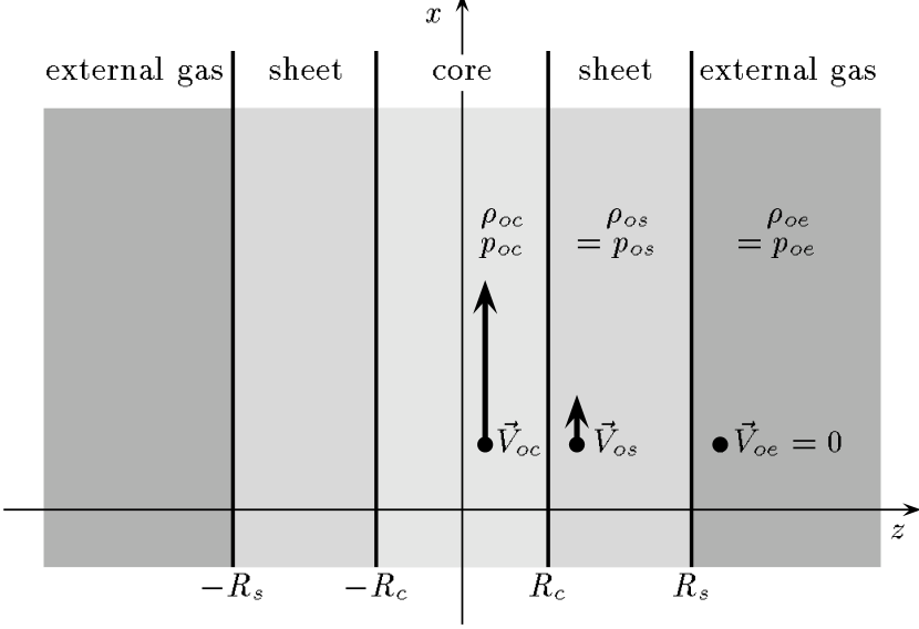
Fig. 1.: Schema of a stratified jet with core, sheet and external components in the unperturbed state.

2 The dispersion relation

We describe the jet with the 2-dimensional slab geometry, which provides an adequate description of the more realistic cylindrical case with respect to the Kelvin-Helmholtz instability (Ferrari et al. 1982). For a large range of physical parameters, the solutions for both the slab and cylindrical cases have similar behaviour, apart from slight numerical differences. This similarity associates the symmetrical and antisymmetrical perturbations of the slab jet with the pinching and helical perturbations of the cylindrical jet respectively. Only high order fluting modes do not have counterparts in slab jets (Ferrari et al, 1982; Hardee, Norman, 1988).

Both spatial and temporal stability analysis of Kelvin-Helmholtz instability have been carried out in the literature. Spatial and convected temporal growth rates have been shown to be not equal but still similar in the two approaches (Hardee, 1986; Norman, Hardee, 1988). This paper investigates the temporal behavior of the instability. We consider a core-sheet jet made of three layers as shown in Fig.1 and describe the transition layers at all interfaces in the vortex-sheet approximation.

The 2-dimensional core-sheet jet initially flows along the $x$-axis on the $x-z$ plane. The unperturbed equilibrium state is defined as follows. $R_{c}$ corresponds to the radius of the inner core, $R_{s}$ to the radius of the surrounding sheet. $V_{o_{c}}$ $(V_{o_{s}},V_{o_{e}})$ is the bulk velocity in the core (respectively the sheet and the external medium), $a_{c}$ the sound velocity in the core, $\rho_{c}$ $(\rho_{s}$, $\rho_{e})$ and $p_{c}$ $(p_{s}$, $p_{e})$ the proper density and pressure in the core (respectively the sheet and the external medium). We also introduce the density contrasts $\nu_{s}={\rho_{o_{c}}/\rho_{o_{s}}}$ and $\nu_{e}={\rho_{o_{s}}/\rho_{o_{e}}}$, where index $o$ stands for unperturbed zero-order values. The relativistic Lorentz factor of the core assumed to be a relativistic gas, the Mach number of the core and the Mach number of sheet are respectively

$$\gamma = \left(1-\frac{V_{o_{c}}^{2}}{c^{2}}\right)^{-1/2},$$ (1)

$$M_{c} = \frac{V_{o_{c}}}{a_{c}},$$ (2)

$$M_{s} = \frac{V_{o_{s}}}{a_{s}}.$$ (3)

We assume that the gas of the sheet moves with a non-relativistic bulk velocity, $V_{o_{s}}\ll c$, and is described by a non relativistic equation of state with adiabatic index $\Gamma_{s}=5/3$, however mildly relativistic sheet could also be taken into account within an analogous way. The external gas is also represented by a nonrelativistic gas with adiabatic index $\Gamma_{e}=5/3$, with $V_{e}=0$ in the unperturbed state.

We shall use the relativistic equation of hydrodynamics in the form applied by Ferrari et al. (1978) for the relativistic core

$$\gamma^{2}\!\!\left(\rho_{c}\!+\!{p_{c}\over c^{2}}\right)\!\!\left[{\partial\mathchoice{\mbox{\boldmath$\displaystyle V$}}{\mbox{\boldmath$\textstyle V$}}{\mbox{\boldmath$\scriptstyle V$}}{\mbox{\boldmath$\scriptscriptstyle V$}}_{c}\over\partial t}\!+\!(\mathchoice{\mbox{\boldmath$\displaystyle V$}}{\mbox{\boldmath$\textstyle V$}}{\mbox{\boldmath$\scriptstyle V$}}{\mbox{\boldmath$\scriptscriptstyle V$}}_{c}\cdotp\mathchoice{\mbox{\boldmath$\displaystyle\nabla$}}{\mbox{\boldmath$\textstyle\nabla$}}{\mbox{\boldmath$\scriptstyle\nabla$}}{\mbox{\boldmath$\scriptscriptstyle\nabla$}})\mathchoice{\mbox{\boldmath$\displaystyle V$}}{\mbox{\boldmath$\textstyle V$}}{\mbox{\boldmath$\scriptstyle V$}}{\mbox{\boldmath$\scriptscriptstyle V$}}_{c}\right]+\mathchoice{\mbox{\boldmath$\displaystyle\nabla$}}{\mbox{\boldmath$\textstyle\nabla$}}{\mbox{\boldmath$\scriptstyle\nabla$}}{\mbox{\boldmath$\scriptscriptstyle\nabla$}}p_{c}+{\mathchoice{\mbox{\boldmath$\displaystyle V$}}{\mbox{\boldmath$\textstyle V$}}{\mbox{\boldmath$\scriptstyle V$}}{\mbox{\boldmath$\scriptscriptstyle V$}}_{c}\over c^{2}}{\partial p_{c}\over\partial t}=0$$ (4)

$$\gamma\left({\partial\rho_{c}\over\partial t}\!+\!\mathchoice{\mbox{\boldmath$\displaystyle V$}}{\mbox{\boldmath$\textstyle V$}}{\mbox{\boldmath$\scriptstyle V$}}{\mbox{\boldmath$\scriptscriptstyle V$}}_{c}\mathchoice{\mbox{\boldmath$\displaystyle\nabla$}}{\mbox{\boldmath$\textstyle\nabla$}}{\mbox{\boldmath$\scriptstyle\nabla$}}{\mbox{\boldmath$\scriptscriptstyle\nabla$}}\rho_{c}\right)\!+\!\left(\rho_{c}+{p_{c}\over c^{2}}\right)\!\!\left[{\partial\gamma\over\partial t}+\mathchoice{\mbox{\boldmath$\displaystyle\nabla$}}{\mbox{\boldmath$\textstyle\nabla$}}{\mbox{\boldmath$\scriptstyle\nabla$}}{\mbox{\boldmath$\scriptscriptstyle\nabla$}}(\gamma\mathchoice{\mbox{\boldmath$\displaystyle V$}}{\mbox{\boldmath$\textstyle V$}}{\mbox{\boldmath$\scriptstyle V$}}{\mbox{\boldmath$\scriptscriptstyle V$}}_{c})\right]=0$$ (5)

and for the non-relativistic sheet gas and external medium,

$${\partial\mathchoice{\mbox{\boldmath$\displaystyle V$}}{\mbox{\boldmath$\textstyle V$}}{\mbox{\boldmath$\scriptstyle V$}}{\mbox{\boldmath$\scriptscriptstyle V$}}_{s,e}\over\partial t}+(\mathchoice{\mbox{\boldmath$\displaystyle V$}}{\mbox{\boldmath$\textstyle V$}}{\mbox{\boldmath$\scriptstyle V$}}{\mbox{\boldmath$\scriptscriptstyle V$}}_{s,e}\mathchoice{\mbox{\boldmath$\displaystyle\nabla$}}{\mbox{\boldmath$\textstyle\nabla$}}{\mbox{\boldmath$\scriptstyle\nabla$}}{\mbox{\boldmath$\scriptscriptstyle\nabla$}})\mathchoice{\mbox{\boldmath$\displaystyle V$}}{\mbox{\boldmath$\textstyle V$}}{\mbox{\boldmath$\scriptstyle V$}}{\mbox{\boldmath$\scriptscriptstyle V$}}_{s,e}+{\mathchoice{\mbox{\boldmath$\displaystyle\nabla$}}{\mbox{\boldmath$\textstyle\nabla$}}{\mbox{\boldmath$\scriptstyle\nabla$}}{\mbox{\boldmath$\scriptscriptstyle\nabla$}}p_{s,e}\over\rho_{s,e}}=0$$ (6)

$${\partial\rho_{s,e}\over\partial t}+\mathchoice{\mbox{\boldmath$\displaystyle\nabla$}}{\mbox{\boldmath$\textstyle\nabla$}}{\mbox{\boldmath$\scriptstyle\nabla$}}{\mbox{\boldmath$\scriptscriptstyle\nabla$}}(\rho_{s,e}\,\mathchoice{\mbox{\boldmath$\displaystyle V$}}{\mbox{\boldmath$\textstyle V$}}{\mbox{\boldmath$\scriptstyle V$}}{\mbox{\boldmath$\scriptscriptstyle V$}}_{s,e})=0\ .$$ (7)

The rest frame density of the relativistic core gas and the enthalpy are respectively

$$\rho_{c} = m_{c}n_{c}+\frac{1}{\Gamma_{c}-1}\frac{p_{c}}{c^{2}},$$ (8)

$$w_{c} = \rho_{c}+\frac{p_{c}}{c^{2}}$$ (9)

where $m_{c}$ and $n_{c}$ are are the rest mass and the number density of gas. The sound speed of relativistic gas is (Taub 1948, Landau & Lifshitz, 1959)

$$a_{c}^{2}=\frac{\Gamma_{c}p_{c}}{w_{c}}$$ (10)

In the ultrarelativistic limit the adiabatic index $\Gamma_{c}={4/3}$, then

$$a_{c}=(\Gamma_{c}-1)^{1/2}c=\frac{c}{\sqrt{3}}.$$ (11)

The Lorentz factor of the core expressed by dimensionless quantities is

$$\gamma=(1-\beta^{2}_{a_{c}}\,M_{c}^{2})^{-1/2},$$ (12)

where $\beta^{2}_{a_{c}}={a_{c}^{2}/c^{2}}={1/3}$.

For the nonrelativistic sheet and external gases we consider equations of state

$$p_{s,e}\rho_{s,e}^{-\Gamma_{s,e}}=p_{o_{s,e}}\,\rho_{o_{s,e}}^{-\Gamma_{s,e}}=\ \hbox{constant}\ ,$$ (13)

with $\Gamma_{s,e}=5/3$, hence

$$\frac{\rho_{s,e}}{\rho_{o_{s,e}}}=\left(\frac{p_{s,e}}{p_{o_{s,e}}}\right)^{1/\Gamma_{s,e}}\ .$$ (14)

The sound speeds of the sheet and external gases are

$$a_{s,e}=\left(\frac{\Gamma_{s,e}p_{s,e}}{\rho_{s,e}}\right)^{1/2}$$ (15)

and the density contrasts can be expressed by sound speed ratios

$$\nu_{s} = {\rho_{o_{c}}\over\rho_{o_{s}}}={{a_{s}}^{2}\over\Gamma_{s}\,a^{2}_{c}},$$ (16)

$$\nu_{e} = \frac{\Gamma_{s}a_{e}^{2}}{\Gamma_{e}a_{s}^{2}}\ .$$ (17)

From now on we shall use dimensionless quantities with sizes scaled to $R_{c}$ and time scaled to ${R_{c}/a_{o_{c}}}$ and introduce the relative pressure perturbations

$$g_{c,s,e}={p_{c,s,e}/p_{o}}$$ (18)

where $p_{o}=p_{o_{c}}=p_{o_{s}}=p_{o_{e}}$.

The equations describing the relativistic core gas can be written as

$$\Gamma_{c}\gamma^{2}g_{c}\left[{\partial\mathchoice{\mbox{\boldmath$\displaystyle V$}}{\mbox{\boldmath$\textstyle V$}}{\mbox{\boldmath$\scriptstyle V$}}{\mbox{\boldmath$\scriptscriptstyle V$}}_{c}\over\partial t}+(\mathchoice{\mbox{\boldmath$\displaystyle V$}}{\mbox{\boldmath$\textstyle V$}}{\mbox{\boldmath$\scriptstyle V$}}{\mbox{\boldmath$\scriptscriptstyle V$}}_{c}\mathchoice{\mbox{\boldmath$\displaystyle\nabla$}}{\mbox{\boldmath$\textstyle\nabla$}}{\mbox{\boldmath$\scriptstyle\nabla$}}{\mbox{\boldmath$\scriptscriptstyle\nabla$}})\mathchoice{\mbox{\boldmath$\displaystyle V$}}{\mbox{\boldmath$\textstyle V$}}{\mbox{\boldmath$\scriptstyle V$}}{\mbox{\boldmath$\scriptscriptstyle V$}}_{c}\right]+\mathchoice{\mbox{\boldmath$\displaystyle\nabla$}}{\mbox{\boldmath$\textstyle\nabla$}}{\mbox{\boldmath$\scriptstyle\nabla$}}{\mbox{\boldmath$\scriptscriptstyle\nabla$}}g_{c}+\beta^{2}_{a_{c}}\,\mathchoice{\mbox{\boldmath$\displaystyle V$}}{\mbox{\boldmath$\textstyle V$}}{\mbox{\boldmath$\scriptstyle V$}}{\mbox{\boldmath$\scriptscriptstyle V$}}_{c}{\partial g_{c}\over\partial t}=0$$ (19)

$$\gamma\left[{\partial g_{c}\over\partial t}+\mathchoice{\mbox{\boldmath$\displaystyle V$}}{\mbox{\boldmath$\textstyle V$}}{\mbox{\boldmath$\scriptstyle V$}}{\mbox{\boldmath$\scriptscriptstyle V$}}_{c}\mathchoice{\mbox{\boldmath$\displaystyle\nabla$}}{\mbox{\boldmath$\textstyle\nabla$}}{\mbox{\boldmath$\scriptstyle\nabla$}}{\mbox{\boldmath$\scriptscriptstyle\nabla$}}g_{c}\right]+\Gamma_{c}\,g_{c}\left[{\partial\gamma\over\partial t}+\nabla(\gamma\mathchoice{\mbox{\boldmath$\displaystyle V$}}{\mbox{\boldmath$\textstyle V$}}{\mbox{\boldmath$\scriptstyle V$}}{\mbox{\boldmath$\scriptscriptstyle V$}}_{c})\right]=0\ .$$ (20)

and the equations of motion for the sheet and the external medium as

$${\partial\mathchoice{\mbox{\boldmath$\displaystyle V$}}{\mbox{\boldmath$\textstyle V$}}{\mbox{\boldmath$\scriptstyle V$}}{\mbox{\boldmath$\scriptscriptstyle V$}}_{s}\over\partial t}+(\mathchoice{\mbox{\boldmath$\displaystyle V$}}{\mbox{\boldmath$\textstyle V$}}{\mbox{\boldmath$\scriptstyle V$}}{\mbox{\boldmath$\scriptscriptstyle V$}}_{s}\mathchoice{\mbox{\boldmath$\displaystyle\nabla$}}{\mbox{\boldmath$\textstyle\nabla$}}{\mbox{\boldmath$\scriptstyle\nabla$}}{\mbox{\boldmath$\scriptscriptstyle\nabla$}})\mathchoice{\mbox{\boldmath$\displaystyle V$}}{\mbox{\boldmath$\textstyle V$}}{\mbox{\boldmath$\scriptstyle V$}}{\mbox{\boldmath$\scriptscriptstyle V$}}_{s}+\nu_{s}\,g_{s}^{-{1\over\Gamma_{s}}}\mathchoice{\mbox{\boldmath$\displaystyle\nabla$}}{\mbox{\boldmath$\textstyle\nabla$}}{\mbox{\boldmath$\scriptstyle\nabla$}}{\mbox{\boldmath$\scriptscriptstyle\nabla$}}g_{s}=0$$ (21)

$${\partial g_{s}^{1\over\Gamma_{s}}\over\partial t}+\mathchoice{\mbox{\boldmath$\displaystyle\nabla$}}{\mbox{\boldmath$\textstyle\nabla$}}{\mbox{\boldmath$\scriptstyle\nabla$}}{\mbox{\boldmath$\scriptscriptstyle\nabla$}}\left(g_{s}^{1\over\Gamma_{s}}\,\mathchoice{\mbox{\boldmath$\displaystyle V$}}{\mbox{\boldmath$\textstyle V$}}{\mbox{\boldmath$\scriptstyle V$}}{\mbox{\boldmath$\scriptscriptstyle V$}}_{s}\right)=0$$ (22)

$${\partial\mathchoice{\mbox{\boldmath$\displaystyle V$}}{\mbox{\boldmath$\textstyle V$}}{\mbox{\boldmath$\scriptstyle V$}}{\mbox{\boldmath$\scriptscriptstyle V$}}_{e}\over\partial t}+(\mathchoice{\mbox{\boldmath$\displaystyle V$}}{\mbox{\boldmath$\textstyle V$}}{\mbox{\boldmath$\scriptstyle V$}}{\mbox{\boldmath$\scriptscriptstyle V$}}_{e}\mathchoice{\mbox{\boldmath$\displaystyle\nabla$}}{\mbox{\boldmath$\textstyle\nabla$}}{\mbox{\boldmath$\scriptstyle\nabla$}}{\mbox{\boldmath$\scriptscriptstyle\nabla$}})\mathchoice{\mbox{\boldmath$\displaystyle V$}}{\mbox{\boldmath$\textstyle V$}}{\mbox{\boldmath$\scriptstyle V$}}{\mbox{\boldmath$\scriptscriptstyle V$}}_{e}+\nu_{s}\nu_{e}\,g_{e}^{-{1\over\Gamma_{e}}}\mathchoice{\mbox{\boldmath$\displaystyle\nabla$}}{\mbox{\boldmath$\textstyle\nabla$}}{\mbox{\boldmath$\scriptstyle\nabla$}}{\mbox{\boldmath$\scriptscriptstyle\nabla$}}g_{e}=0$$ (23)

$${\partial g_{e}^{1\over\Gamma_{e}}\over\partial t}+\mathchoice{\mbox{\boldmath$\displaystyle\nabla$}}{\mbox{\boldmath$\textstyle\nabla$}}{\mbox{\boldmath$\scriptstyle\nabla$}}{\mbox{\boldmath$\scriptscriptstyle\nabla$}}\left(g_{e}^{1\over\Gamma_{e}}\,\mathchoice{\mbox{\boldmath$\displaystyle V$}}{\mbox{\boldmath$\textstyle V$}}{\mbox{\boldmath$\scriptstyle V$}}{\mbox{\boldmath$\scriptscriptstyle V$}}_{e}\right)=0$$ (24)

The linearization of (19) and (21) leads to

$$\gamma^{2}\Gamma_{c}\left({\partial\over\partial t}+M_{c}{\partial\over\partial x}\right)V^{\prime}_{c_{z}}+{\partial g^{\prime}_{c}\over\partial z}=0$$ (25)

$$\gamma^{2}\Gamma_{c}\left({\partial\over\partial t}+M_{c}{\partial\over\partial x}\right)V^{\prime}_{c_{x}}+\left({\partial\over\partial x}+\beta^{2}_{a_{c}}\,M_{c}{\partial\over\partial t}\right)g^{\prime}_{c}=0$$ (26)

$${1\over\nu_{s}}\left({\partial\over\partial t}+M_{s}\sqrt{\nu_{s}\Gamma_{s}}{\partial\over\partial x}\right)V^{\prime}_{s_{z}}+{\partial g^{\prime}_{s}\over\partial z}=0$$ (27)

$${1\over\nu_{s}\nu_{e}}\left({\partial\over\partial t}+M_{s}\sqrt{\nu_{s}\Gamma_{s}}{\partial\over\partial x}\right)V^{\prime}_{s_{x}}+{\partial g^{\prime}_{s}\over\partial x}=0$$ (28)

$${1\over\nu_{s}\nu_{e}}{\partial V^{\prime}_{e_{z}}\over\partial t}+{\partial g^{\prime}_{e}\over\partial z}=0$$ (29)

$${1\over\nu_{s}\nu_{e}}{\partial V^{\prime}_{e_{x}}\over\partial t}+{\partial g^{\prime}_{e}\over\partial x}=0$$ (30)

in the rest frame of the external medium, where prime denotes first order perturbed quantities. Combining (25), (26) and linearized (20) gives

$$\left.{\partial^{2}g^{\prime}_{c}\over\partial z^{2}}+\gamma^{2}\right[ - \left({\partial\over\partial t}+M_{c}{\partial\over\partial x}\right)^{2}$$ (31)

$$+ \left({\partial\over\partial x}+\left.\beta^{2}_{a_{c}}\,M_{c}{\partial\over\partial t}\right)^{2}\right]g^{\prime}_{c}=0$$

while combining linearized (22) with (27) and (28) for the sheet and with (29) and (30) for the external medium gives

$${\partial^{2}g^{\prime}_{s}\over\partial z^{2}}+\left[{\partial^{2}\over\partial x^{2}}-{1\over\nu_{s}\Gamma_{s}}\left({\partial\over\partial t}+M_{s}\sqrt{\nu_{s}\Gamma_{s}}{\partial\over\partial x}\right)^{2}\right]g^{\prime}_{s}=0$$ (32)

and

$${\partial^{2}g^{\prime}_{e}\over\partial z^{2}}+\left[{\partial^{2}\over\partial x^{2}}-{1\over\nu_{s}\nu_{e}\Gamma_{e}}{\partial^{2}\over\partial t^{2}}\right]g^{\prime}_{e}=0\ .$$ (33)

Let us assume in the core and the sheet perturbations of the form (for $z>0$)

$$\delta^{\prime}_{c,s}=[\delta^{+}_{c,s}F^{+}_{c,s}(z)+\delta^{-}_{c,s}F^{-}_{c,s}(z)]\exp i(k_{x}x-\omega t)+c.c.$$ (34)

where $F^{\pm}_{c,s}(z)=\exp(\pm i\,k_{{c_{z},s_{z}}}z)$ allow to describe waves propagating in opposite $z$-directions. Perturbations in the external medium are of the form

$$\delta^{\prime}_{e}=\delta^{+}_{e}F^{+}_{e}(z)\exp\,i(k_{x}x-\omega t)+c.c.$$ (35)

where $F^{+}_{e}(z)=\exp\,i\,k_{e_{z}}z$ represents only outgoing waves for positive $z$. Here $k_{x}$ is the parallel wavenumber longitudinal to the jet and $k_{c_{z}}$ (respectively $k_{s_{z}}$ and $k_{e_{z}}$) is the transverse wavenumber perpendicular to the jet axis in the core region (respectively in the sheet and external regions). The transverse wavenumbers $k_{c_{z}}$, $k_{s_{z}}$ and $k_{e_{z}}$ are complex since the perturbations we consider represent surface waves.

For a temporal stability analysis, $k_{x}$ is real and $\omega$ complex. Equations (31), (32) and (33) lead to

$$k_{c_{z}} = \left(\omega^{2}_{c_{o}}-k^{2}_{x_{o}}\right)^{1/2}$$ (36)

$$k_{s_{z}} = \left({\omega^{2}_{s_{o}}\over\nu_{s}\Gamma_{s}}-k_{x}^{2}\right)^{1/2}$$ (37)

$$k_{e_{z}} = \left({\omega^{2}\over\nu_{s}\nu_{e}\Gamma_{e}}-k_{x}^{2}\right)^{1/2}$$ (38)

where $\omega_{c_{o}}=\gamma(\omega-M_{c}k_{x})$ and $k_{x_{o}}=\gamma(k_{x}-\beta^{2}_{a_{c}}M_{c}\omega)$ are the frequency and wavenumber in the rest frame of the core fluid and $\omega_{s_{o}}=\omega-\sqrt{\nu_{s}\Gamma_{s}}M_{s}k_{x}$ is the frequency in the rest frame of the sheet fluid. From equations (10), (27) and (29) we deduce the relations

$$V^{\prime\pm}_{c_{z}} = {\pm k_{c_{z}}\over\Gamma_{c}\gamma\,\omega_{c_{o}}}\,G^{\prime\pm}_{c}$$ (39)

$$V^{\prime\pm}_{s_{z}} = {\pm\nu_{s}k_{s_{z}}\over\omega_{s_{o}}}\,G^{\prime\pm}_{s}$$ (40)

$$V^{\prime+}_{e_{z}} = {\nu_{s}\nu_{e}k_{e_{z}}\over\omega}\,G^{\prime+}_{e}$$ (41)

Symmetry conditions of the problem allow to consider only half-space with $z\geq 0$. The components $(+)$ and $(-)$ propagate respectively in the positive and negative $z$-direction. Our perturbation takes into account only outgoing solution in the external medium.

The dispersion relation of the system is obtained from the boundary conditions at the internal (core/sheet) and external (sheet/external gas) interfaces, namely pressure equilibrium and equality between the $z$-component of the gas displacement and the transversal displacement of contact surface. In the reference frame of the core gas, this condition writes

$$v^{(c)^{\prime}}_{c_{z}}-{\partial\over\partial t^{(c)}}h^{(c)^{\prime}}_{c}=0$$ (42)

We call $h^{\prime}_{c}$ and $h^{\prime}_{s}$ the transversal displacements of core/sheet and sheet/external surfaces. The exponent $(c)$ stands for values determined in the core gas rest frame. From Lorentz transformation

$$v^{(c)^{\prime}}_{c_{z}}=\frac{v_{c_{z}}^{\prime}\sqrt{1-\beta^{2}_{a_{c}}M_{c}^{2}}}{1-\beta^{2}_{a_{c}}(M_{c}+v^{\prime}_{c_{x}})M_{c}}\ ,$$ (43)

which reduces to $v^{(c)^{\prime}}_{c_{z}}=\gamma v_{c_{z}}^{\prime}$ in the linear approximation. Moreover

$${\partial\over\partial t^{(c)}}=\gamma\left({\partial\over\partial t}+M_{c}{\partial\over\partial x}\right)$$ (44)

and $h^{\prime}_{c}$, the displacement of surface, is Lorentz invariant as well as the pressure $g^{\prime}_{c}$. Boundary conditions at the internal interface located at $z=1$ become

$$v^{\prime}_{c_{z}} - \left({\partial\over\partial t}+M_{c}{\partial\over\partial x}\right)h^{\prime}_{c}=0$$ (45)

$$v^{\prime}_{s_{z}} - \left({\partial\over\partial t}+\sqrt{\nu_{s}\Gamma_{s}}M_{s}{\partial\over\partial x}\right)h^{\prime}_{c}=0$$ (46)

$$g^{\prime}_{c} = g^{\prime}_{s}$$ (47)

and at the external interface located at $z=R$ $(\equiv{R_{s}/R_{c}})$,

$$v^{\prime}_{s_{z}} - \left({\partial\over\partial t}+\sqrt{\nu_{s}\Gamma_{s}}M_{s}{\partial\over\partial x}\right)h^{\prime}_{s}=0$$ (48)

$$v^{\prime}_{e_{z}} - {\partial\over\partial t}h^{\prime}_{s}=0$$ (49)

$$g^{\prime}_{s} = g^{\prime}_{e}\ .$$ (50)

Fig. 2.: Temporal growth rate of the antisymmetric solution for an underdense core and sheet jet, for fundamental mode (top), first reflection mode (middle) and second reflection mode (bottom). $R=R_{s}/R_{c}=2$, $5$ and $10$ for first, second and third columns. Dotted lines correspond to a single jet case with no sheet and $R=1$, while dashed lines correspond to a single jet case with no external component and $R=\infty$ (infinite sheet). Parameters are $\gamma=10$, $M_{s}=0$, $\nu_{c}=\rho_{c}/\rho_{s}=0.01$ and $\nu_{s}=\rho_{s}/\rho_{e}=0.1$

Fig. 3.: Same as Fig. 2 but here $\nu_{c}=0.01$ and $\nu_{s}=10$

Fig. 4.: Same as Fig.2 and 3 but here $\nu_{c}=0.1$ and $\nu_{s}=0.001$

We can take the forms of the transversal displacements as follows

$$h^{\prime}_{c,s}=A_{c,s}\exp\,i\,(k_{x}x-\omega t)+c.c.$$ (51)

After substitutions and elimination of $A_{c,s}$, we reach the general dispersion relation for core-sheet jets

$$\left({Z_{s}\over Z_{c}}\right)\ {F^{+}_{s}(1)+{\cal R}_{se}F^{+}_{s}(2R-1)\over F^{+}_{s}(1)-{\cal R}_{se}F^{+}_{s}(2R-1)}={F^{+}_{c}(1)+\varepsilon F^{-}_{c}(1)\over F^{+}_{c}(1)-\varepsilon F^{-}_{c}(1)}$$ (52)

which leads to

$${Z_{s}\over Z_{c}}\left[{1+{\cal R}_{se}e^{2ik_{s_{z}}(R-1)}\over 1-{\cal R}_{se}e^{2ik_{s_{z}}(R-1)}}\right]=\left\{\matrix{{\rm coth}\ ik_{c_{z}}\quad{\rm for}\ \varepsilon=1\cr{\rm or}\cr{\rm th}\ ik_{c_{z}}\qquad{\rm for}\ \varepsilon=-1\cr}\right.$$ (53)

where we have used the fact that by definition $F^{+}_{s}(R)F^{-}_{s}(1)/F^{-}_{s}(R)=F^{+}_{s}(2R-1)$ and have imposed the conditions of symmetry or antisymmetry of the solutions, $G^{-}_{c}=\varepsilon G^{+}_{c}$ with $\varepsilon=\pm 1$. We introduce the complex normal acoustic impedances (Payne & Cohn 1985) for the core, sheet and external medium, which after elimination of factors constant across all the components can be expressed as

$$Z_{c} = \Gamma_{c}\omega^{2}_{c_{0}}/k_{c_{z}},$$ (54)

$$Z_{s} = \omega^{2}_{s_{0}}/(\nu_{s}k_{s_{z}}),$$ (55)

$$Z_{e} = \omega^{2}/(\nu_{s}\nu_{e}k_{e_{z}}).$$ (56)

The reflection and transmission coefficients at core-sheet and sheet-external gas interfaces are respectively defined as

$${\cal R}_{cs}=\frac{Z_{s}-Z_{c}}{Z_{s}+Z_{c}}, {\cal T}_{cs}=\frac{2Z_{s}}{Z_{s}+Z_{c}}$$ (57)

$${\cal R}_{se}=\frac{Z_{e}-Z_{s}}{Z_{e}+Z_{s}}, {\cal T}_{se}=\frac{2Z_{e}}{Z_{e}+Z_{s}}$$ (58)

When there is no reflection at this external boundary (interface sheet-external), ${\cal R}_{se}=0$ and the effect of the external gas disappears. Equations (53) reduce to the case of a single jet with internal medium corresponding to the core component and external medium to the sheet component. Another way to cancel the effect of external gas is to assume a very large sheet since the factor of ${\cal R}_{se}$ in (53) vanishes as $\exp[-2R\,\rm Im(k_{s_{z}})]$ for $R>>1$. A stratified jet with infinite sheet therefore corresponds to a single jet with only core and sheet components. Conversely, for $R=1$, internal and external interfaces coincide and equations (53) reduce again to the case of a single jet, but then with only core component and external gas.

3 Numerical results and their physical interpretation

The method used to solve the dispersion relation (53) is based on the Newton-Raphson method (Press et al, 1992). Different sets of parameters have been investigated. They all lead to the same qualitative results.

1. The presence of the sheet induces an oscillating pattern on the growth rate diagram

2. The stability properties are dominated by the sheet even if its thickness is comparable with the core radius.

3. The amplitude of oscillations of growth rate diminish with increasing sheet thickness.

This is well illustrated in Figs.2 to 4 which show the temporal growth rate of the antisymmetric fundamental, first and second reflection modes of core and sheet jets.

The apparent oscillating pattern is a new feature caused by the reflections of acoustic waves at the interface between sheet and external gas. These reflections are represented by the reflection coefficient ${\cal R}_{se}$ in dispersion relation (53). The wave radiated at the core-sheet ($cs$) interface toward the sheet layer is reflected from the sheet-external ($se$) interface and next returns to the ($cs$) interface as shown in Fig.5. Thus, one can expect resonances due to the presence of the sheet component if

$$\Delta\phi=2n\pi,$$ (59)

where $\Delta\phi$ is the change of phase of sound wave in sheet on the path between $cs$, $se$ and $cs$ interfaces and $n$ is an integer number. Introducing the length of path of the wave between $cs$ and $se$ interfaces (see Fig.5)

$$L=\frac{R-1}{\cos\alpha},$$ (60)

where $\alpha$ is the wave propagation angle defined by $\ tg\alpha=k_{x}/k_{s_{z}}$, and the wavelength

$$\lambda_{s}=2\pi/\sqrt{k^{2}_{x}+k^{2}_{s_{z}}}$$ (61)

we can write the resonant condition (59) in explicit form

$$2L=n\lambda_{s}\ ,$$ (62)

The above interpretation of the oscillating pattern is demonstrated in Fig.6., where we presented again the solution of Fig.4 in the linear scale. The superimposed high bars represent these values of $k_{x}$ (one should remember that $k_{s_{z}}$ is a function of $k_{x}$) for which the condition (62) is fulfilled. For comparison, the small bars represent these $k_{x}$ for which we have an antiresonance

$$2L=\left(n+\frac{1}{2}\right)\lambda_{s}\ ,$$ (63)

We can easily notice a coincidence of the maxima of growth rate with high bars and minima with small bars, what proves the validity of our physical interpretation. In a case of external gas which is significantly lighter then the sheet gas we notice ${\cal R}_{se}\simeq-1$ (the change of phase by $\pi$) resulting in a reversed relation between bars and the maxima of growth rate. This effect is remarkable comparing Figs.2 and 3, where maxima and minima in both the figures are inverted. Figure 5 shows a clear coincidence of maxima, minima and bars described above. Varying the parameters of the core sheet configuration we observe however that the bars can be shifted uniformly with respect to maxima and minima toward smaller or larger $k_{x}$ values. This is not a surprise since all the reflection and transmission coefficients are complex quantities in general and the additional phase shifts are natural for each reflection at the interfaces.

The entire interaction of sound waves at the core-sheet interface appears to be very complicated. The normal acoustic impedances $Z_{c}$ and $Z_{s}$ depend on both real and oscillating imaginary parts of $\omega$ and $k_{c,s_{z}}$. As Payne & Cohn (1985) shown the instability coincides with vanishing (in practice small) values of denominator in expression for the reflection and transmission coefficients. In the case of core-sheet interface we have $Z_{c}\simeq-Z_{s}$ and even relatively small oscillations of these quantities result in strong oscillations of ${\cal R}_{cs}$ and ${\cal T}_{cs}$ around the averaged values typical for the sheet layer of infinite thickness. Both the reflected and transmitted waves at the ($cs$) interface come back to this interface after a finite number of cycles returning the acoustic energy which has already been radiated in both directions. This returned energy results in the modified growth rate of the instability and again the growth rate influence the reflection and transmission coefficients at the ($cs$) interface. Because of the multiplicity of interfaces, many waves interfere within the core-sheet jet configuration and the detailed description of these interactions seems to be a difficult task.

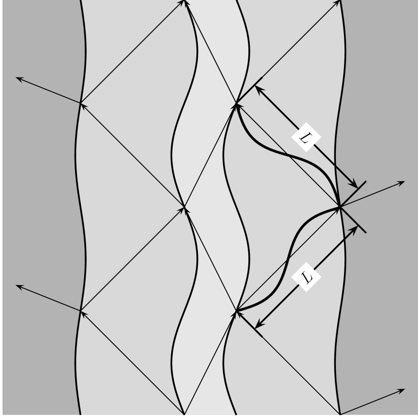
Fig. 5.: The physical interpretation of the effect of oscillating growth rate is as follows: The sound wave emitted at the internal interface first reflects at the external interface and then returns to the internal interface and interferes with the new emitted wave. The waves drawn within the sheet layer demonstrate the integer number of wave periods between interfaces, not the way of deformation of sheet (the acoustic waves are longitudinal waves). The case $L=\lambda_{s}$ is shown.

Fig. 6.: The maxima of the growth rate coincide with the integer multiples of wavelength on the path of the acoustic wave. We show the growth rate versus wavenumber k in the linear scale for the case presented in Fig.4 (fundamental mode, R = 5). The high bars located below the curve of growth rate indicate the fulfillment of the resonance condition (62) and the small bars indicate the fulfillment of the antiresonance condition (63)

We explored different sets of values for the densities, Lorentz factor of the core and Mach number of the sheet, for antisymmetric or symmetric solutions. In all chosen cases, $|{\cal R}_{se}|$ remains smaller than 1, implying that no magnification of the waves occurs at the external interface. Variation of the sheet Mach number slightly shifts the oscillating pattern but does not modify the average growth rate as long as the sheet keeps a classical velocity. This statement is valid also in the case of sheet velocity exceeding the sheet sound speed ($M_{s}>1$) as long as we assume that the core is relativistic and sheet is nonrelativistic. The main source of the instability comes from the internal interface where amplification of the waves can take place. Generally speaking, the instability develops due to the interaction between the core and the sheet, with the oscillatory modification superimposed by the presence of the external ($se$) interface.

For small $k_{s_{z}}$, when the effective thickness of the sheet is smaller than the half-wavelength, namely $\lambda_{s}>2(R-1)/\cos\alpha$ the growth rate for the stratified case resembles to the solution obtained for a single jet without sheet $(R=1)$ or appears as a kind of compromise between the two extreme cases of no sheet or infinite sheet.

For all studied sets of parameters, the temporal growth rate of the stratified jet instability tends to the solution obtained for the case of an infinite sheet or oscillates around it for large $k_{s_{z}}$ (corresponding to large $k_{x}$). Oscillations are always reduced while increasing the sheet thickness. Practically all solutions that we obtained converge to the case of infinite sheet as soon as $R$ reaches the order of 5 and often even less. So the presence of a sheet with a thickness of only a few times the core component radius imposes the growth rate of the instability. It is the physical parameters of the sheet relatively to the core medium which are decisive for the growth of the instability instead of the parameters of the external medium. An illustration of this is provided by Fig.2 and Fig.3 which show almost similar growth rate for the stratified scenario (except for the inversion of the maxima and minima) in spite of different values of the density ratio $\nu_{e}=\rho_{s}/\rho_{e}$.

4 Astrophysical implications

The effect of the sheet that we study in the 2-dimensional slab geometry corresponds to the effect due to an envelope, a sheath or a cocoon around the jet in the cylindrical description. The general result that properties of the sheet essentially influence the linear growth of the Kelvin-Helmholtz instability have several consequences.

It shows that the maximal growth rate and corresponding wavenumber can be modified by the presence of even a modest envelope. This is illustrated by the case of Fig.4, where an envelope not very different from the core-component (same thickness with $R=2$, density ratio of $\rho_{c}/\rho_{s}=0.1$) induces an increase of $\omega_{I}^{\max}$ from 0.03 to 0.2 and of $k^{\max}_{x}$ from 0.1 to 1 for the fundamental mode. The linear growth of the helical mode of such a jet is therefore much faster and the resonant wavelength decreases to about $6R_{c}$. Such modification due to the new complexity driven by the envelope-effect can help to solve some difficulties encountered when trying to deduce parameters such as densities and temperatures from the radio morphology of jets, under the assumption that knots and wiggles are respectively due to the growth of pinching and helical modes (Ferrari et al, 1983; Zaninetti, Van Horn, 1988). Indeed, the parameters deduced in such studies for the external medium can be considered as applying only to an envelope surrounding the jet, with density and temperature possibly quite different from values deduced for instance from X-rays data on intergalactic gas. However the model of core-sheet jet is complex and involves much more free parameters which makes any model-dependent predictions more difficult.

The determination of physical parameters of astrophysical jets based on the model of Kelvin – Helmholtz instability is a challenge, but it is also made difficult by our lack of detailed knowledge on the nonlinear evolution of the instability. Several authors investigated the nonlinear regime by means of numerical simulations (e.g. Hardee et al. 1992, Bodo et al. 1994) in the case of nonrelativistic jets and applying analytical methods (Hanasz 1995) in the case of relativistic jets. The last approach shows that in the phase preceding the formation of shock waves within the relativistic jet, the growth of instability slows down while the perturbation amplitude grows and finally the growth is stopped for the amplitude of lateral displacement of the jet which is only a fraction of the jet radius. The physical reasons responsible for this behaviour can be summarized as a strong nonlinear growth of modulus of the acoustic impedances of both the internal (relativistic) and the surrounding (nonrelativistic) gases, associated with the growth of perturbation amplitude. The properties of the surrounding gas and the presence or absence of the sheet layer are important for the properties of the Kelvin-Helmholtz instability in this aspect as well. The numerical simulations allow to trace the evolution of perturbations up to the jet disruption. As Bodo et al. (1994) shown the time interval between the formation of first shock waves and the beginning of the mixing phase is dependent on the values of the Mach number of the jet and the density contrast. According to this work the smaller density and higher Mach number jets can survive in the form of laminar flow for a longer time. We would like to point out that in analogy to our previous results we can expect that the parameters of sheet in the case of stratified jets will control the life time of the laminar flow.

Coming back to the linear approximation we point out that the presence of an envelope underdense relatively to the external medium tends to induce faster growth of the instability while overdense envelope slows it down. The high stability of a large number of radio jets can therefore be better understood if dense and cool envelopes are commonly present, as expected in “multilevel” or two-component jet models (Smith, Raine, 1985; Baker et al, 1988; Sol et al, 1989; Achatz et al, 1990). This could explain for instance the remarkable stability of the inner jet of the wide-angle tail (WAT) radio source 3C465. This source is hosted by the central galaxy of the cluster of galaxies Abell 2634. A hot intercluster gas makes the external medium in which the radio jet propagates. X-ray observations provided estimates of its temperature and density with distance to the core, $T_{e}\simeq 2\times 10^{7}$K and $n_{e}\simeq 8\times 10^{-4}(p^{+}e^{-})$cm^-3 at 20kpc (Eilek et al, 1984). From Faraday rotation measures, Leahy (1984) suggested the existence of thermal plasma inside the jet with a density of $10^{-2}(p^{+}e^{-})$cm^-3 in the inner hot spots at about 20kpc from the core and of $5\times 10^{-4}(p^{+}e^{-})$cm^-3 on average in the tails. We tentatively identify this thermal plasma with the sheet component of our study (indeed in our description, the slow plasma of the sheet can also be present at $z<R_{c}$, with the fast-moving plasma of the core just streaming through it). In two-flow models, the slow component (here the sheet or envelope) is made by a collimated wind coming from the accretion disc. Assuming that its temperature is comparable to or less than the one of the gas in the disc at the basis of the outflow, one can expect a temperature in the range $10^{4}-10^{6}$K for the envelope, from the temperature variation proposed by Phinney (1989) in the accretion discs. Taking $T_{s}\hbox{\raise 2.15277pt\hbox{$<$} \kern-11.00008pt\lower 2.15277pt\hbox{$\sim$}}10^{6}$ required $n_{s}\hbox{\raise 2.15277pt\hbox{$>$} \kern-11.00008pt\lower 2.15277pt\hbox{$\sim$}}1.6\times 10^{-2}(p^{+}e^{-})$cm^-3 in the region of the inner hot spots to ensure pressure equilibrium with the intercluster gas at the external interface. Such values of $n_{s}$ are quite in agreement with the Faraday rotation analysis and correspond to an overdense envelope which tends to stabilize the inner jet structure.

Such type of envelopes could be present in many other extragalactic radio sources as proposed in an application of two-component jet models (Dole et al, 1995) and as suggested by the “tomography” analysis of radio data (Rudnick, 1995). Direct estimates of the envelope densities are not yet available. However the sheath detected by Katz-Stone and Rudnick (1994) around the jet of the FRII source Cygnus A corresponds to an enhancement of the density of radiating particles, and therefore likely to an increase of the thermal plasma density as well. Overdense sheaths would influence the dynamics of FRII jets and increase their stability. A somewhat analogous role was already known to be played by FRII cocoons. Indeed numerical simulations emphasized the importance of a cocoon for the dynamics of FRII jets (Norman et al, 1984a,b) and identified two regimes, mode-dominated or cocoon-dominated. Our study deal with laminar flows and can not precisely describe FRII-cocoons which are turbulent. However it proposes some theoretical interpretation of the cocoon-dominated regime observed in numerical experiments. Our results are analogous to the results obtained by Hardee & Norman (1990), who notice that the jet dynamics is determined by properties of the jet and lobe, but not by the properties in the undisturbed medium. In their numerical simulations the lobe surrounds the jet in a manner resembling to our sheet or envelope. In fact, four different layers can be expected in such cases, namely the inner jet, the sheath, the cocoon and the external media. From our results on core-sheet jets, we tentatively infer that the stability properties of this highly stratified configuration will be dominated by the Kelvin-Helmholtz instability of the most unstable interface, likely the internal one if the inner jet is relativistic, slightly modified by the multiple reflections of the acoustic waves at the other interfaces.

The question of the origin of sheaths or envelopes around extragalactic jets is still open. They can just emanate from the inner jets as the result of particle diffusion. This could concern the slow-moving radio “cocoon” of the jet in 3C273. The interaction itself between the jet and its surroundings induces turbulent sheared and entrainment layers which can lead to the formation of sheaths for instance in FRI sources. In FRII sources, the backflow from the hot spots constitutes some kind of sheaths as well, as already mentioned. Other possibilities proposed by two-component models for jets are to generate stratified jets, inner cores and surrounding sheaths, directly from the central engines. In all these cases, the presence of an envelope with thickness comparable or slightly larger than the central jet radius deeply modifies the interaction of the jet with the ambient medium of the host galaxy, and somewhat isolates the jet from its surroundings. This makes then rather problematic to explain the dichotomy between radio-loud and radio-quiet objects by the difference in the media where the jets have to propagate. Such an argument of difference in the host galaxy interstellar medium is often proposed to account for the fact that well-developed radio jets are observed in elliptical galaxies but not in spiral and Seyfert galaxies, based on the idea that jets are rapidly destroyed by their interaction with the dense and inhomogeneous interstellar gas expected in spiral galaxies. In fact, the interstellar medium can influence the radio source evolution in two ways, first by its direct interaction with the jet, second by its primordial role during the accretion process. Our results favour the latter option since the former one appears easily inhibited by specific internal jet properties. Within such a view, the dichotomy between radio-loud and radio-quiet objects should arise from specific properties of the central engine possibly acquired during its formation and accretion phase.

• This project was partially supported by PICS/CNRS no.198 “Astronomie Pologne”.

References

- 1 Achatz, U., Lesch, H., Schlickeiser, R., 1990, A&A, 233, 391.
- 2 Achatz, U., Schlickeiser, R., 1992, Extragalactic radio sources –from beams to jets, Roland, J., Sol, H., Pelletier, G., ed., Cambridge University Press, p.256.
- 3 Bahcall, J.N., Kirhakos, S., Schneider, D.P., Davis, R.J., Muxlow, T.W.B., Garrington, S.T., Conway, R.G., Unwin, S.C., 1995, ApJ, 452, L91.
- 4 Baker, D.N., Borovsky, J.E., Benford, G., Eilek, J.A., 1988, ApJ, 326, 110.
- 5 Biretta, J.A., Zhou, F., Owen F.N., 1995, ApJ, 447, 582.
- 6 Birkinshaw, M., 1991, Beams and jets in Astrophysics, P.A. Hughes, ed., Cambridge University Press, p.278.
- 7 Bodo, G., Massaglia, S., Ferrari, A., Trussoni, E., 1994, A&A, 283, 655
- 8 Chan, K.L., Henriksen, R.N., 1980, ApJ, 241, 534.
- 9 Dole, H., Sol, H., Vicente, L., 1995, IAU Symposium 175 ‘Extragalactic Radio Sources’ (Bologna).
- 10 Eilek, J.A., Burns, J.O., O’Dea, C.P., Owen, F.N., 1984, ApJ, 278, 37.
- 11 Ferrari, A., Trussoni, E., Zaninetti,L., 1978, A&A, 64, 43
- 12 Ferrari, A., et al, 1982, MNRAS, 198, 1065.
- 13 Ferrari, A., et al, 1983, A&A, 125, 179.
- 14 Hanasz, M., 1995, PhD Thesis, Nicolaus Copernicus University, Torun.
- 15 Hardee, 1986, ApJ, 303, 111.
- 16 Hardee, P.E., Norman, M.L., 1988, ApJ, 334, 70
- 17 Hardee, P.E., Norman, M.L., 1990, ApJ, 365, 134
- 18 Hardee, P.E., Cooper, M.A., Norman, M.L., Stone, J.M. 1992, ApJ, 399, 478
- 19 Katz-Stone, D.M., Rudnick, L., Anderson, M.C., 1993, ApJ, 407, 549.
- 20 Katz-Stone, D.M., Rudnick, L., 1994, ApJ, 426, 116.
- 21 Königl, A., Kartje, J.F., 1994, ApJ, 434, 446.
- 22 Landau, L.D., Lifshitz, E.M., 1959, Fluid Mechanics, Pergamon Press, Oxford.
- 23 Leahy, J.P., 1984, MNRAS, 208, 323.
- 24 Melia, F., Königl, A., 1989, ApJ, 340, 162.
- 25 Norman, M.L., Smarr, L.L. and Winkler, K.-H.A., 1984a in Numerical Astrophysics: A Festschrift in Honor of James R. Wilson, ed. R. Bowers, J. Centrella, J. Leblanc and M. Leblanc (Jones and Bartlett: Boston).
- 26 Norman, M.L., Winkler, K.-H.A., Smarr, L.L., 1984b in Physics of Energy Transport in Extragalactic Radio Sources, eds A.H. Bridle and J.A.Eilek, NRAO, p. 150
- 27 Norman, M.L., Hardee, P.E., 1988, ApJ, 334, 80.
- 28 O’Donoghue, A.A., Owen, F.N., Eilek, J.A., 1990, ApJ, 72, 75.
- 29 O’Donoghue, A.A., Owen, F.N., Eilek, J.A., 1993, ApJ, 408, 428.
- 30 Payne, D.G., Cohn, H., 1985, ApJ, 291, 655.
- 31 Pelletier, G., Sol, H., 1992, MNRAS, 254, 635.
- 32 Phinney, E.S., 1989, Theory of accretion disks, Meyer, F., Duschl, W.J., Frank, J., Meyer-Hofmeister, E., ed., Kluwer Academic Publishers, p.457.
- 33 Press, W.H., Flannery, B.P., Teukolsky, S.A., Vetterling, W.T., 1992, Numerical recipes, Cambridge University Press.
- 34 Rudnick, L., Katz-Stone, D.M., Anderson, M.C., 1994, ApJSuppl. Ser., 90, 955.
- 35 Rudnick, L., 1995, IAU Symposium 175 ‘Extragalactic Radio Sources’ (Bologna).
- 36 Smith, M.D., Raine, D.J., 1985, MNRAS, 212, 425.
- 37 Sol, H., Pelletier, G., Asséo, E., 1989, MNRAS, 237, 411.
- 38 Taub, A.H., 1948, Phys. Rev. 74, 328
- 39 Zaninetti, Van Horn, 1988, A&A, 189, 45.