The Palomar Distant Cluster Survey :
III. The Colors of the Cluster Galaxies

Abstract

We present a color analysis of the galaxy populations of candidate clusters of galaxies from the Palomar Distant Cluster Survey (Postman et al. 1996). The survey was conducted in two broad band filters that closely match $V$ and $I$ and contains a total of 79 candidate clusters of galaxies, covering an estimated redshift range $0.2\mathrel{\hbox{\raise 2.15277pt\hbox{$<$}\hbox to0.0pt{\hss\lower 2.15277pt\hbox{$\sim$}}}}z\mathrel{\hbox{\raise 2.15277pt\hbox{$<$}\hbox to0.0pt{\hss\lower 2.15277pt\hbox{$\sim$}}}}1.2$. We examine the color evolution in the 57 richest clusters from this survey, the largest statistical sample of distant clusters to date. The intermediate redshift ($0.2\mathrel{\hbox{\raise 2.15277pt\hbox{$<$}\hbox to0.0pt{\hss\lower 2.15277pt\hbox{$\sim$}}}}z\mathrel{\hbox{\raise 2.15277pt\hbox{$<$}\hbox to0.0pt{\hss\lower 2.15277pt\hbox{$\sim$}}}}0.4$) clusters show a distinct locus of galaxy colors in the color–magnitude diagram. This ridge line corresponds well with the expected no–evolution color of present–day elliptical galaxies at these redshifts. In clusters at redshifts of $z\mathrel{\hbox{\raise 2.15277pt\hbox{$>$}\hbox to0.0pt{\hss\lower 2.15277pt\hbox{$\sim$}}}}0.5$, this red envelope has shifted bluewards compared to the “no–evolution” prediction. By $z\sim 0.8$ there are only a few galaxies which are as red in their rest-frame as present–day ellipticals, consistent with recent claims on the basis of optical–infrared colors. The detected evolution is consistent with passive aging of stellar populations formed at redshifts of $z\mathrel{\hbox{\raise 2.15277pt\hbox{$>$}\hbox to0.0pt{\hss\lower 2.15277pt\hbox{$\sim$}}}}2$.

Though the uncertainties are large, the Butcher–Oemler effect is observed in the Palomar clusters. The fraction of blue galaxies increases with the estimated redshift of the cluster at a 96.2% confidence level. The measured blue fractions of the intermediate redshift clusters ($f_{b}\sim 0.2-0.3$) are consistent with those found previously by Butcher & Oemler (1984). The trend in the Palomar clusters suggests that $f_{b}$ can be greater than 0.4 in clusters of galaxies at redshifts of $z\mathrel{\hbox{\raise 2.15277pt\hbox{$>$}\hbox to0.0pt{\hss\lower 2.15277pt\hbox{$\sim$}}}}0.6$.

Accepted for publication in the Astronomical Journal

Subject headings: galaxies: clusters of galaxies; cosmology: observations; evolution

1 Introduction

The study of the galaxy populations of rich clusters provides important constraints on the formation mechanisms of both clusters and galaxies. Present–day clusters show a distinct correlation between the structure of the cluster and the galaxy population. Irregular, open clusters, such as Virgo, are spiral–rich. These systems show no obvious condensations, though the galaxy surface density is at least five times as great as the surrounding field ($n_{\rm gal}>30~{}h^{3}~{}{\rm galaxies~{}{Mpc}^{-3}}$). These clusters may be highly assymetric and have significant degrees of substructure. Dense, centrally concentrated clusters, such as Coma, contain predominantly early–type galaxies in their cores (Abell 1958; Oemler 1974; Dressler 1980; Postman & Geller 1984). These clusters have a single, outstanding concentration among the bright member galaxies and typically display a high–degree of spherical symmetry. Central densities can reach as high as $10^{4}~{}h^{3}~{}{\rm galaxies~{}{Mpc}^{-3}}$. The galaxy content of clusters is part of the general morphology–density relation of galaxies; as the local density increases, the fraction of elliptical (E) and S0 galaxies increases, while the fraction of spiral galaxies decreases (Dressler 1980; Postman & Geller 1984).

One of the most intriguing results of the study of intermediate and high–redshift clusters of galaxies has been strong evolution in the galaxy population. Butcher & Oemler (1984; hereafter BO) were the first to make a comprehensive study of intermediate redshift clusters with regard to their galaxy populations. They examined the fraction of blue galaxies ($f_{b}$) in 33 clusters at $z\mathrel{\hbox{\raise 2.15277pt\hbox{$<$}\hbox to0.0pt{\hss\lower 2.15277pt\hbox{$\sim$}}}}0.5$. They found that $f_{b}$ is an increasing function of redshift in both open and compact clusters of galaxies, indicating that clusters at these redshifts are significantly bluer than their low–redshift counterparts. Recent HST image data (Dressler et al. 1994; Couch et al. 1994; Oemler, Dressler & Butcher 1996) reveal that many of these blue ($g-r<1.2$) galaxies are either “normal” spirals or have peculiar morphologies, producing non–elliptical fractions which are 3 to 5 times higher than the average current epoch cluster. Fading through cessation of star formation may play a role in this evolution. Gunn & Dressler (1988) find that the spectra of cluster galaxies with $z\mathrel{\hbox{\raise 2.15277pt\hbox{$>$}\hbox to0.0pt{\hss\lower 2.15277pt\hbox{$\sim$}}}}0.6$ show, on average, smaller 4000$\AA$ decrements and a higher frequency of post–starburst features (the “E+A” spectral class) than those at $z<0.6$ (however, see Zabludoff et al. 1996).

Detailed photometric observations of other intermediate redshift ($z\mathrel{\hbox{\raise 2.15277pt\hbox{$<$}\hbox to0.0pt{\hss\lower 2.15277pt\hbox{$\sim$}}}}0.4$) clusters have confirmed the original results of BO. Even though these clusters show an increased fraction of blue galaxies, they still contain a population of E/S0s which distinguish itself by extremely red colors and a tight color–magnitude (CM) relation (a “red envelope”). Both the mean color and the CM relation is consistent with that of present–day ellipticals (Sandage 1972; Visvanathan & Sandage 1977; Butcher & Oemler 1978; Couch & Newell 1984; BO; Ellis et al. 1985; Sandage, Bingelli & Tammann 1985; Millington & Peach 1990; Aragón-Salamanca, Ellis & Sharples 1991; Luppino et al. 1991; Dressler & Gunn 1992; Le Borgne, Pelló & Sanahuja 1992; Dressler et al. 1994; Molinari et al. 1994; Smail, Ellis & Fitchett 1994; Stanford, Eisenhardt & Dickinson 1995).

Aragón-Salamanca et al. (1993; hereafter A93) have studied a small sample of 10 rich clusters at $0.5<z<0.9$ in the optical–infrared colors. They observe an increase in the number of blue members which they interpret as the high–redshift extension to the Butcher–Oemler effect. This trend is also well studied by Rakos & Schombert (1995) in an intermediate and high–redshift sample of 17 rich clusters. They find the fraction of blue galaxies increases from 20% at $z=0.4$ to 80% at $z=0.8$ using Strömgren photometry in the cluster rest-frame. In addition, the red envelope, presumably that of the early–type population, moves bluewards with redshift (A93; Rakos & Schombert 1995; Oke, Gunn & Hoessel 1996). At $z\sim 0.9$, there are few cluster members with colors as red as present–day ellipticals (see also Smail et al. 1994). The color distribution of this high-redshift elliptical population is relatively narrow, and the trend is uniform from cluster to cluster; this suggests a homogeneous population which formed within a narrow time span (e.g. Bower, Lucey & Ellis 1992a,b). Dickinson (1995) finds similar results in a cluster of galaxies which is associated with the $z=1.206$ radio galaxy 3C 324. The galaxies exhibit a narrow, red locus in the CM magnitude diagram. This branch is $\sim 0.6$ mag bluer than the expected “no–evolution” value, though the intrinsic rms color scatter is only 0.2 mag. The observed color trend for the red envelope of galaxies is consistent with passive evolution of an old stellar population formed by a single burst of star formation at redshifts of $z\mathrel{\hbox{\raise 2.15277pt\hbox{$>$}\hbox to0.0pt{\hss\lower 2.15277pt\hbox{$\sim$}}}}2$. The reasonably small color scatter would imply closely synchronized intra–cluster star formation (Bower et al. 1992a,b; A93; Dickinson 1995).

It is critical to test the claims of significant color evolution in high–redshift clusters of galaxies against larger, more statistically complete samples. In this paper, we examine the galaxy colors of the largest, statistically complete sample of distant clusters presently available, the Palomar Distant Cluster Survey (hereafter PDCS; Postman et al. 1996). This sample of 57 distant clusters will be used to trace the color evolution in the galaxy population and to investigate the Butcher–Oemler effect in clusters up to a redshift of $\sim 1$. In §2 of this paper, we briefly describe the PDCS, the original photometric reduction, and the cluster sample used in this analysis. The evolution in the color distributions of the cluster galaxies is presented in §3. The Butcher–Oemler effect (the fraction of blue galaxies as a function of redshift) is presented in §4. We summarize the results in §5.

2 The Data

The observations, data reduction, and cluster catalog are the subject of the first paper in this series (Postman et al. 1996; hereafter Paper I). However, we discuss briefly the aspects of the original survey which are necessary for the following analysis. The cluster sample is derived from an optical/near IR survey with the 4–shooter CCD camera on the Palomar 5 meter telescope. The survey covers five fields, each of which is approximately one degree square. The five regions will be denoted as the ${00}^{{\rm h}}$, ${02}^{{\rm h}}$, ${09}^{{\rm h}}$, ${13}^{{\rm h}}$, and ${16}^{{\rm h}}$ fields.

2.1 The Photometry

The Palomar Distant Cluster Survey was conducted in two broad band filters, the F555W and F785LP of HST’s Wide Field/Planetary Camera. We denote these bands $V_{4}$ (F555W) and $I_{4}$ (F785LP) according to the convention in Paper I. The response curves of these filters are shown in Fig. 1 of Paper I. The rough transformations to the $V$ band and the Kron-Cousins $I_{KC}$ band are given by

$$V = V_{4}-0.02-0.056~{}(V_{4}-I_{4})+0.012~{}{(V_{4}-I_{4})}^{2}$$ (1)

$$I_{KC} = I_{4}-0.43+0.089~{}(V_{4}-I_{4})$$ (2)

Photometric conversions to other standard photometric systems are given in Paper I. The zero points of the $V_{4}$ and $I_{4}$ magnitudes are based on the AB magnitude system of Oke & Gunn (1983). The data are complete to roughly $V_{4}^{iso}=23.8$ and $I_{4}^{iso}=22.5$ in the isophotal magnitudes. The estimated uncertainties in the FOCAS photometry are $\pm 0.12$ mag for a galaxy with $V_{4}^{iso}=22.0$ and $I_{4}^{iso}=21.0$. The zero point fluctuations from field to field are estimated at $\mathrel{\hbox{\raise 2.15277pt\hbox{$<$}\hbox to0.0pt{\hss\lower 2.15277pt\hbox{$\sim$}}}}0.07$ mag (see Paper I for details).

The object detection and classification was performed with a modified version of FOCAS (Jarvis & Tyson 1981; Valdes 1982). The basic FOCAS object detection, point spread function (PSF), measurement, deblending, and star–galaxy–noise classification algorithms are used. The $V_{4}$ and $I_{4}$ band CCD images are analyzed individually. The object isophotal detection threshold in each frame is set to be $3\sigma_{sky}$ (typically 25.7 mag per ${\rm arcsec^{2}}$ in the $V_{4}$ band and 24.8 mag per ${\rm arcsec^{2}}$ in the $I_{4}$ band), and a minimum object size requirement of 15 pixels (1.68 ${\rm arcsec^{2}}$) is imposed. The sky background is defined as the mode of values in a given region surrounding the isophotal limits of the galaxy. Because the sky level is lower, and the system response is higher in the $V_{4}$ band than in the $I_{4}$ band, the $V_{4}$ images are deeper. Consequently, about 40% of the objects detected in a typical $V_{4}$ image are undetected by FOCAS in the corresponding $I_{4}$ image. Nearly all of these objects are faint (isophotal magnitude of $V_{4}^{iso}\mathrel{\hbox{\raise 2.15277pt\hbox{$>$}\hbox to0.0pt{\hss\lower 2.15277pt\hbox{$\sim$}}}}23$). About 95% of the objects with $\mathrel{\hbox{\raise 2.15277pt\hbox{$<$}\hbox to0.0pt{\hss\lower 2.15277pt\hbox{$\sim$}}}}23$ are detected in both bands.

In the following analysis, we use those objects which have been classified as galaxies by the FOCAS algorithm in the band where the object is brightest. The object classification accuracy is discussed extensively in §3.3 of Paper I. The classifier breaks down for objects fainter than about 1 magnitude above the completeness limit. Near the limit, the signal-to-noise is low ($S/N\sim 4$), and the mean object area is $\mathrel{\hbox{\raise 2.15277pt\hbox{$<$}\hbox to0.0pt{\hss\lower 2.15277pt\hbox{$\sim$}}}}5\times{\rm FWHM^{2}}$, making reliable classification difficult. This effect may mean that some distant ellipticals (those galaxies that we specifically want to examine) are misclassified as stars. However, because galaxies outnumber stars by about 7 to 1 at the magnitude limit of the sample, this is not a significant effect (see Figs. 7 & 8 of Paper I). In addition, we have confirmed that the results of this paper remain unchanged even if we had included the stars in the color analysis and simply subtracted them through the statistical field subtraction (see §3).

For the color analysis in this paper, we have obtained aperture photometry on all galaxies detected individually in the $V_{4}$ and $I_{4}$ bands as described above. A circular aperture of 5.03 arcsec in radius was used. This corresponds to a physical size of $\{13.8~{}19.1~{}21.1\}~{}h^{-1}~{}{\rm kpc}$ at $z=\{0.3~{}0.6~{}0.9\}$. The aperture magnitude limits are $V_{4}^{ap}\approx 22.8$ and $I_{4}^{ap}\approx 21.4$. The uncertainty in the ${(V_{4}-I_{4})_{ap}}$ color is estimated at $\sim 0.2$ mag for a galaxy close to our aperture magnitude limits. In the analysis which follows, we assume $q_{o}=0.5~{}{\rm and}~{}H_{o}=100~{}h~{}{\rm km~{}s^{-1}~{}Mpc^{-1}}~{}{\rm with}~{}h=0.75$.

2.2 The Cluster Sample

A matched filter algorithm was used to objectively identify the cluster candidates by using positional and photometric data simultaneously. This technique is likely to be more robust than previous optical selections which simply looked for surface density enhancements, a method which can be significantly affected by superposition effects (e.g. Abell 1958; Gunn, Hoessel & Oke 1986; Couch et al. 1991). An advantage of this technique is that redshift estimates of the cluster candidates are produced as a byproduct of the matched filter; the main disadvantage is that we must assume a particular form for the cluster luminosity function (for the flux filter) and cluster radial profile (for the radial filter). The radial filter $P(r)$ and the flux filter $L(m)$ are given by

$$P(r)= {1\over{\sqrt{1+(r/r_{c})^{2}}}}-{1\over{\sqrt{1+(r_{co}/r_{c})^{2}}}} r<r_{co}$$ if (3)

$$0$$ otherwise

$$L(m)={{\phi(m-m^{*})~{}10^{-0.4(m-m^{*})}}\over{b(m)}}$$ (4)

$P(r)$ is an azimuthally symmetric cluster surface density profile which has a characteristic core radius ($r_{c}$) and which falls off at large radii as $r^{-1}$. The function is explicitly cut off at an arbitrary cutoff radius ($r_{co}$). We have chosen $r_{c}=100~{}h^{-1}~{}{\rm kpc}$ and $r_{co}=10\times r_{c}$ such that the radial profile resembles the profiles of nearby clusters and that we have optimized the cluster detections relative to the spurious detection rates (Paper I). $b(m)$ is the background galaxy counts. $\phi(m-m^{*})$ is the differential Schechter luminosity function with $\alpha=-1.1$ and $M^{*}=-21.0$ and $-21.9$ in the $V_{4}$ and $I_{4}$ bands, respectively; here, we assume the shape of the luminosity function is independent of redshift and adopt a k–correction appropriate for a non–evolving elliptical galaxy (see Fig. 1). For the derivation of these filters and a detailed explanation, see Paper I. We have used extensive Monte–Carlo simulations in Paper I and Lubin & Postman (1996; hereafter Paper II) to quantify the selection function due to the functional form of the matched filter. We find that the selection bias has a minimal effect on the properties of the observed clusters. We can detect clusters with a broad range of profile shapes, luminosity function parameters, and color evolution (Paper I; Paper II).

The catalog consists of 79 candidate clusters of galaxies detected with estimated redshifts between $0.2\leq z_{est}\leq 1.2$. The estimated redshifts are determined at discrete 0.1 intervals and represent the redshift at which the cluster candidate best matches the filter. The uncertainty in the estimated redshift ($z_{est}$) is $\sigma_{z_{est}}\mathrel{\hbox{\raise 2.15277pt\hbox{$<$}\hbox to0.0pt{\hss\lower 2.15277pt\hbox{$\sim$}}}}0.2$. This value is determined from both the simulations and those clusters in the survey which have measured redshifts. Presently, only 10% of the cluster sample have reliably measured redshifts, although they span almost the entire range in redshift, $0.3<z_{obs}<1.1$. In all cases, the estimated redshifts are within $z_{obs}\pm 0.2$ (see Fig. 15 and §4.2.1 of Paper I). The redshift survey of the Palomar clusters is ongoing, and those interested in its current status should contact the authors.

Candidate clusters are detected individually in each band and then matched with the other to locate those systems which are detected in both bands. 87% of the cluster candidates are matched detections; that is, they have been significantly detected in both the $V_{4}$ and $I_{4}$ bands. The amplitude of the matched filter provides an estimate of the cluster richness. This filter richness ($\Lambda_{cl}$) is a measure of the effective number of $L^{*}$ galaxies in the cluster (see §4.2.2 of Paper I; Lubin 1995). Through Monte–Carlo simulations, we can statistically determine the relation between $\Lambda_{cl}$ and the actual cluster richness as determined by the specification of Abell (1958). This relation is dependent on profile shape; as the cluster profile slope steepens, a given $\Lambda_{cl}$ value corresponds to a lower richness class. For a cluster which has a surface density profile of approximately $r^{-1.4}$ (the average profile of the PDCS clusters; Paper II), $\Lambda_{cl}\mathrel{\hbox{\raise 2.15277pt\hbox{$>$}\hbox to0.0pt{\hss\lower 2.15277pt\hbox{$\sim$}}}}40$ corresponds to Abell ${\rm R}\geq 1$ (Paper I). Therefore, in the analysis which follows, we will examine only those clusters which have been significantly detected in both bands with $\Lambda_{cl}\geq 40$ in either of the two bands. This corresponds to a sample of 57 clusters. We list in Table 1 the cluster ID # and the estimated redshift ($z_{est}$) and filter richness parameter ($\Lambda_{cl}$) as determined in the passband where the significance of the detection is highest (see Paper I).

3 Color Evolution

In the following analysis, we use the color–magnitude (CM) diagram and the color distribution to examine the color evolution in the PDCS cluster galaxies as a function of redshift. Though it is difficult to select a morphological class based solely on a single broad–band color, we have tried to identify the high–redshift counterparts to nearby ellipticals and S0s by looking for their distinct locus or “red envelope” in the CM diagram of clusters. At $z\mathrel{\hbox{\raise 2.15277pt\hbox{$<$}\hbox to0.0pt{\hss\lower 2.15277pt\hbox{$\sim$}}}}0.4$, the E/S0 population in clusters has colors which are negligibly different from their present–day counterparts (see §1). At higher redshifts, there is a systematic and monotomic evolution as a function of redshift in the optical-infrared colors of early-type galaxies in clusters (A93; Rakos & Schombert 1995; Oke et al. 1996). At $z\sim 0.9$ there are few cluster galaxies as red as present–day ellipticals (A93; Dickinson 1995; Rakos & Schombert 1995).

We examine these trends in the $V_{4}$ and $I_{4}$ bands of the PDCS sample of intermediate and high redshift clusters of galaxies. On an individual cluster basis, we are limited by statistics and the uncertainty in the estimated redshift ($z_{est}$); therefore, we follow the same approach as in Paper II and create global cluster composites for our color analysis. Because the cluster redshifts have an estimated uncertainty of $\sigma_{z_{est}}\mathrel{\hbox{\raise 2.15277pt\hbox{$<$}\hbox to0.0pt{\hss\lower 2.15277pt\hbox{$\sim$}}}}0.2$ (see §2.2 and §4.2.1 of Paper I), we sort the cluster sample by estimated redshift into three broad redshift ranges : (1) $0.2\leq z_{est}\leq 0.4$, (2) $0.5\leq z_{est}\leq 0.7$, and (3) $0.8\leq z_{est}\leq 1.2$. $z_{est}$ is determined in discrete 0.1 redshift intervals (see Paper I). Table 2 lists the number of PDCS clusters per redshift interval in each of the five fields.

In examining the color data, we adhere to the convention of displaying the observed colors for the galaxies in our intermediate and high–redshift cluster samples; that is, we do not reduce our data to their zero–redshift equivalent by applying k–corrections. In making comparisons to present–day populations of cluster galaxies, we have dimmed appropriately the current epoch data (see §3.1).

3.1 No Evolution Predictions

In order to compare our observations with those at zero redshift, we calculate the color evolution of typical nearby galaxies of various morphological type assuming “no evolution.” We have used the spectral energy distributions (SEDs) from Coleman, Wu & Weedman (1980) and calculated the $V_{4}$ and $I_{4}$ k–corrections and expected $V_{4}-I_{4}$ colors as a function of redshift and morphological type (see also Frei & Gunn 1994; Fukugita, Shimasaku & Ichikawa 1995). Fig. 1 shows the results of these calculations. The correction to the galaxy color due to the relative change in projected linear size of the photometric aperture is small compared to other uncertainties ($\mathrel{\hbox{\raise 2.15277pt\hbox{$<$}\hbox to0.0pt{\hss\lower 2.15277pt\hbox{$\sim$}}}}0.05~{}{\rm mag}$; Sandage & Visvanathan 1978; Silva & Elston 1994).

Because we are trying to assess the color evolution in the cluster galaxies over a broad range in redshift, we need to quantify our selection biases due to the magnitude limit of our survey. Therefore, we have created a no–evolution simulation by examining a “synthetic” cluster population over our redshift range. We have constructed this population from CL 0939+4713 ($z=0.41$) which has galaxies with measured colors and morphological classifications from HST (Dressler et al. 1994). Dressler et al. (1994) found that this cluster exhibited a blue fraction consistent with that expected from the Butcher–Oemler effect. The colors of the cluster galaxies suggest that most of them are normal examples of their Hubble type, and their luminosity functions are consistent with that of present–day cluster galaxies. We have converted the $g$ and $r$ magnitudes of Dressler & Gunn (1992) to the $V_{4}$ and $I_{4}$ bands (see Paper I for photometric conversions). Fig. 2 shows the color–magnitude diagram and color distribution of this simulated no-evolution galaxy population as a function of redshift. We have chosen the redshifts $z=\{0.3~{}0.6~{}0.9\}$ because they are roughly the medians of the 3 estimated redshift intervals being studied here. When calculating the aperture magnitude ($I_{4}^{ap}$) at these redshifts, we have taken into account the change in projected linear size of the photometric aperture with redshift; however, we have not corrected the $V_{4}-I_{4}$ colors for the effect of a color gradient as the correction is small (see Sandage & Visvanathan 1978; Silva & Elston 1994).

The E/S0s (filled circles) appear on a distinct locus in each of these diagrams. Fig. 2 also shows the total color distribution (solid line histogram) and the distribution that we would be observed given the magnitude limits of our survey (shaded histogram). In order to compare the actual data with these evolutionary predictions, we need a quantitative description of these color distributions. We would like an estimator of the mean color (presumably that of the early–type population) which is not severely affected by the presence of a blue tail. We follow the approach used in A93 and adopt the biweight location ($C_{BI}$) and scale ($S_{BI}$) estimators (Beers, Flynn & Gebhardt 1990 and references therein). These estimators are well-suited to non-Gaussian distributions. For a Gaussian distribution, $C_{BI}$ is better than 80% efficient at accurately determining the mean with more than 10 points, while $S_{BI}$ asymptotically approaches the standard deviation (see Beers et al. 1990 for exact details). In order to gauge the $1\sigma$ errors on these parameters, we have used a bootstrap analysis. This technique involves randomly drawing many new samples (of equal number) from the original sample of galaxy colors. The standard deviations of the resulting parameter distributions are defined as the $1\sigma$ parameter errors. Table 3 lists these parameters for the total and observed color distributions of the simulated cluster populations. The more conventional descriptors, the median and interquartile range, give results which are similar to those of the biweight location and scale estimators.

Fig. 2 shows that, at $z=0.3$, the simulated color distributions are unaffected by the magnitude limit of the survey. At $z=0.6$, the E/S0 population still appears as a clear peak in the color distribution ($V_{4}$ – $I_{4}$ $\sim 2.2$), even though a large portion of the cluster population extends beyond the magnitude limits of the survey. At $z\sim 0.9$, the observed color distribution (bottom panels of Fig. 2) is significantly altered, though it would still be possible to detect the brightest cluster ellipticals at $I_{4}^{ap}\mathrel{\hbox{\raise 2.15277pt\hbox{$<$}\hbox to0.0pt{\hss\lower 2.15277pt\hbox{$\sim$}}}}20$ with a predicted color of ${(V_{4}-I_{4})}_{ap}\sim 3$. The mean color in this redshift interval is $C_{BI}\sim 2.4$. Note that the differential k-correction (Fig. 1) causes a distinct change in the relative number of E/S0s versus spirals observed in the different redshift bins. For the chosen synthetic cluster population, the ratio of E/S0s to spirals is $\sim 3$; this ratio is preserved in the observed color distribution of a cluster at $z\sim 0.3$ but becomes $\sim 1$ for a cluster at $z\sim 0.9$.

For the analysis of the PDCS clusters, we study composite color distributions (see §3.2). Since we co-add clusters over a broad range in redshifts, this will artificially increase the dispersion around the elliptical color–magnitude relation, as well as the width of the color distribution in general. For example, from $z=0.2\rightarrow 0.4$ the no–evolution elliptical color changes by $\sim$ 0.6 mag (Fig. 1). We simulate this effect by generating the synthetic cluster population of Fig. 2 at random redshifts between $0.1\mathrel{\hbox{\raise 2.15277pt\hbox{$<$}\hbox to0.0pt{\hss\lower 2.15277pt\hbox{$\sim$}}}}z\mathrel{\hbox{\raise 2.15277pt\hbox{$<$}\hbox to0.0pt{\hss\lower 2.15277pt\hbox{$\sim$}}}}1.2$. We then create composite color diagrams for each redshift interval such that we have roughly the same number of galaxies as observed in the PDCS composites (see Fig. 7). These, therefore, are the color distributions that we would expect in our survey if the galaxy populations are non–evolving. The resulting distributions for the simulated cluster population are shown in Fig. 3. No background contamination is included in this figure. Table 4 lists the biweight location and scale estimators and their $1\sigma$ uncertainties for these distributions. The mean color as measured by the biweight location estimator remains the same within the measurement error as the distributions in Fig. 2; as expected, the dispersion, as characterized by the biweight scale estimator, increases by up to 15%.

3.2 Composite Color Distributions of the Palomar Clusters

We now examine the color distributions of the 57 PDCS clusters. For each cluster candidate, we examine all of the galaxies within $0.5~{}h^{-1}~{}{\rm Mpc}$ of the cluster center. The composite CM diagrams are shown in Fig. 4. We plot the aperture color $(V_{4}-I_{4})_{ap}$ versus the aperture $I_{4}^{ap}$ magnitude. We have made composite CM diagrams separately for each of the five fields. The top three rows show the composites for each of the three redshift intervals. These plots include both cluster and background galaxies. The bottom row of Fig. 4 shows the CM diagrams for regions of the five fields which contain no detected clusters (indicated as “field”). Extinction corrections (see Paper I) have been applied. In these diagrams, we have not corrected $I_{4}^{ap}$ for the change in projected linear size of the photometric aperture over each redshift interval because of the redshift uncertainty. This correction corresponds to $\mathrel{\hbox{\raise 2.15277pt\hbox{$<$}\hbox to0.0pt{\hss\lower 2.15277pt\hbox{$\sim$}}}}0.30,~{}0.08$ and $0.03$ mag in the three respective intervals. The correction due to color gradients in $B-V$ is small; this translates into correction of $\mathrel{\hbox{\raise 2.15277pt\hbox{$<$}\hbox to0.0pt{\hss\lower 2.15277pt\hbox{$\sim$}}}}0.05$ mag in the $V_{4}-I_{4}$ color (Sandage & Visvanathan 1978; Silva & Elston 1994).

In Fig. 5, we have combined the data of each PDCS field (Fig. 4) to make composite color–magnitude diagrams for each of the three redshift intervals. Even though we are contaminated by background galaxies, it is clear that the CM diagram for the lowest redshift interval (top row) shows a distinct locus of galaxies centered at $(V_{4}-I_{4})_{ap}=1.2\pm 0.2$ and extending to magnitudes as bright as $I_{4}^{ap}\sim 16$. This distinct feature is not clearly observed in the higher redshift intervals (second and third rows). The envelope in the lowest redshift interval corresponds well with the color expected for a non–evolving early–type population.

Fig. 6 shows the corresponding color distributions for each of the PDCS fields before (solid line histograms) and after (shaded histograms) a statistical correction for background. Each cluster color distribution was background subtracted using the background color distribution determined from all regions of the field which contain no detected clusters (bottom row of Fig. 6). The “field” regions of the $02^{\rm h}$ field contain slightly fewer galaxies because a larger fraction of the field is excluded because either the $V_{4}$ or $I_{4}$ band data does not exist. We have co-added the background–corrected color distributions of each PDCS field (Fig. 6) to make a global cluster composites for each redshift interval. Fig. 7 shows the resulting distributions in each of the three redshift intervals. The bar in each panel indicates the range of expected (no–evolution) elliptical/S0 colors over this redshift interval (see Fig. 1). Fig. 7 clearly reveals that we do not see the expected effect of the large k–correction.

Since we cannot distinguish these galaxies morphologically, we use the biweight location estimator as a representation of the mean galaxy color and, presumably, the population of early–type galaxies. Table 5 lists the biweight location ($C_{BI}$) and scale estimator ($S_{BI}$) for these distributions. We have perturbed the expected field contamination by $\pm 1\sigma$ and recomputed the distribution characteristics. The resulting parameters are all within $1\sigma$ of the original estimators in Table 5, indicating that we are not adversely affected by the background subtraction.

As indicated in Fig. 7 and Table 5, there is a distinct peak at $(V_{4}-I_{4})_{ap}\sim 1.3$ for clusters in the range $0.2\leq z_{est}\leq 0.4$. This color corresponds well to the expected no–evolution color of present–day ellipticals at these redshifts (Fig. 1). The distribution of colors in this redshift interval is reasonably consistent with that expected from our simulations of the no–evolution composite color distribution of a synthetic cluster population (Fig. 3 and Table 3). The results of the PDCS clusters are also typical of other intermediate redshift clusters of galaxies where a ridge line of early type galaxies, with colors similar to that of present–day ellipticals, is obvious in the CM diagrams and color distributions (BO; Couch & Newell 1984; Millington & Peach 1990; Aragón-Salamanca et al. 1991; Luppino et al. 1991; Dressler & Gunn 1992; Le Borgne et al. 1992; Dressler et al. 1994; Molinari et al. 1994; Smail et al. 1994).

Comparing our no–evolution predictions shown in Fig. 3 to the resulting color distributions of the Palomar clusters shown in Fig. 7, we see a distinct difference in the two highest redshift intervals. In the interval $0.5\leq z_{est}\leq 0.7$, the mean color of the PDCS cluster galaxies is $(V_{4}-I_{4})_{ap}\sim 1.6$. From the no–evolution simulations of §3.1, we would expect a clear peak near $(V_{4}-I_{4})_{ap}\sim 2$ (Fig. 3). The “red envelope” has apparently moved bluewards by $\sim 0.4$ mag. In the interval $0.8\leq z_{est}\leq 1.2$, there are only a few ($\sim 5$) galaxies which are as red as present–day ellipticals ($V_{4}-I_{4}\sim 3$ at these redshifts). The mean color, $(V_{4}-I_{4})_{ap}\sim 1.2$, is bluer by $\sim 1.2$ mag than that predicted in the no–evolution simulated cluster population (Table 4). If the mean color is an accurate representation of the colors of the early–type cluster population, this result indicates that these galaxies are significantly bluer than the no–evolution predictions. This color distribution may, however, be adversely influenced by two effects. Firstly, late–type cluster members at high redshift would be preferentially detected in the optical passbands. This may mean that the characteristic color is artificially bluer; however, this effect is unlikely to account for the large color difference between our data and the no–evolution predictions (compare Figs. 3 & 7). Secondly, as we only have estimated redshifts for most of the cluster sample, there is the possibility that some of these high–redshift clusters are actually superpositions of poor groups or clusters along the line-of-sight. Since there are only 5 clusters in the highest redshift bin (Table 2), a misclassification of a few of these cluster candidates would make the resulting color distribution significantly bluer. Because of this possibility and the substantial threat of contamination at these redshifts, we have used the Kolmogorov-Smirnov (KS) test to confirm that the two high-redshift samples are not consistent with being drawn from the field population. The probability that the two color distributions are drawn from the field population is less than 0.002%.

In addition, we have explored a different approach in defining the samples in the two highest redshift bins. We have imposed different magnitude limits such that we are complete for the likely ${(V_{4}-I_{4})}_{ap}$ colors of the early-type cluster population. These limits are $I_{4}^{ap}=20.5$ in the $0.5\leq z_{est}\leq 0.7$ redshift interval and $I_{4}^{ap}=20.0$ in the $0.8\leq z_{est}\leq 1.2$ redshift interval. For a cluster at $z\sim 0.9$, the new $I_{4}^{ap}$ magnitude limit should greatly improve the accurate identification of the red cluster members (bottom left panel of Fig. 2). From the new samples, we have created composite color distributions in the same manner as described above. The biweight location and scale estimators for the resulting color distributions are $C_{BI}=1.71\pm 0.07$ and $S_{BI}=0.51\pm 0.05$ ($0.5\leq z_{est}\leq 0.7$) and $C_{BI}=1.29\pm 0.15$ and $S_{BI}=0.70\pm 0.10$ ($0.8\leq z_{est}\leq 1.2$). The mean colors are reasonably consistent within the measurement uncertainty with the results of the original analysis; however, they are slightly redder as expected if this technique improves our identification of the red cluster galaxies. Still, the mean colors are bluer than the no–evolution predictions of the synthetic cluster populations by $\sim 0.3$ mag at $z\sim 0.6$ and $\sim 1.1$ mag at $z\sim 0.9$, respectively.

The estimated redshift distribution of the Palomar clusters is examined in Paper I. This distribution is consistent with the hypothesis that the typical, bright distant cluster galaxy is bluer than a non–evolving elliptical at the cluster redshift. This further supports the results of the color analysis presented here.

The observed blueing trend in the Palomar clusters has also been observed by Rakos & Schombert (1995) in the rest-frame Strömgren $uvby$ filters and by A93 in the optical–infrared colors. A93 examined 10 rich clusters at $0.5<z<0.9$ and found that the red envelope is bluer than present–day ellipticals by approximately 0.4, 0.5, and 1.3 mag in $V-K$ at the mean redshifts of $\langle z\rangle=0.56,~{}0.70,~{}{\rm and}~{}0.88$, respectively. Based on the simple Bruzual & Charlot (1996) evolutionary models presented in §3.3, the observed $V-K$ color differences would imply a color shift (relative to the no-evolution prediction) in the $V_{4}-I_{4}$ color of roughly $0.4(\pm 0.2)$ and $1.0(\pm 0.2)$ at $z=0.6$ and $0.9$, respectively. These predictions are consistent within the photometric and measurement errors with the observed color evolution in the Palomar clusters.

3.3 Comparison with Evolutionary Models

Aragón-Salamanca et al. (1993), Dickinson (1995), and Rakos & Schombert (1995) have all noted that the observed evolutionary trend in clusters at $z\mathrel{\hbox{\raise 2.15277pt\hbox{$>$}\hbox to0.0pt{\hss\lower 2.15277pt\hbox{$\sim$}}}}0.4$ is consistent with simple passive evolution of an old stellar population which was originally formed in a single burst of star-formation at an epoch of $z\mathrel{\hbox{\raise 2.15277pt\hbox{$>$}\hbox to0.0pt{\hss\lower 2.15277pt\hbox{$\sim$}}}}2$ (see also Bower et al. 1992a,b; Charlot & Silk 1994; Pehre et al. 1995; Ellis et al. 1996). We examine these conclusions by comparing the results of our color analysis to the population synthesis models of Bruzual & Charlot (e.g. Bruzual 1983; Bruzual & Charlot 1993, 1996 and references therein). The free parameters in these models are the initial mass function (IMF) and the star formation rate (SFR). We choose the traditional Scalo (1986) IMF with lower and upper mass limits of 0.1 and 125 $M_{\odot}$, respectively. For the SFR, we explore two possible rates : (1) a burst of constant star formation for a initial period $\tau$ ($c$–model; Bruzual 1983); and (2) an exponentially decaying SFR such that a fraction $\mu=1-e^{-1{\rm Gyr}/\tau}$ of the galaxy mass is converted into stars after the first Gyr ($\mu$–model; Bruzual 1983). The evolutionary calculations have been made using the Bruzual & Charlot (1996) synthesis code. The age of the galaxy is determined by the redshift ($z_{f}$) at which the epoch of star formation began. We relate look-back time to redshift using $H_{o}=75~{}{\rm km~{}s^{-1}~{}Mpc^{-1}}$ and $q_{o}=\{0.0~{}0.5\}$.

In Fig. 8, we show the results for two models with (1) $\tau=1~{}{\rm Gyr}$ and (2) $\mu=0.5$ for three formation epochs of $z_{f}=\{1~{}2~{}10\}$. Given the large redshift uncertainty, the color evolution in the Palomar clusters is consistent with passive evolution of a single burst of star formation at $z_{f}\approx 2$. Both models provide a reasonable fit to the color evolution at $z\mathrel{\hbox{\raise 2.15277pt\hbox{$<$}\hbox to0.0pt{\hss\lower 2.15277pt\hbox{$\sim$}}}}0.6$, implying formation epochs of $z_{f}\mathrel{\hbox{\raise 2.15277pt\hbox{$>$}\hbox to0.0pt{\hss\lower 2.15277pt\hbox{$\sim$}}}}2$. Previous observations of distant clusters in the optical–infrared colors indicate similar formation epochs (A93; Dickinson 1995; Rakos & Schombert 1995).

The $\mu$–model provides a better fit to the data in the highest redshift bin as more evolution is predicted at $z\sim 0.9$. As noted in §3.2, since optical passbands at high-redshift sample the rest-frame UV light which is most affected by recent bursts of star formation, the color distribution in the highest redshift bin will be biased toward late-type cluster galaxies. Therefore, the characteristic (or mean) color of this distribution may not accurately represent the early-type cluster population but may actually be bluer. This would, of course, affect how well a particular model fits the optical colors. In light of this, we have examined a combination of evolutionary models representing a mix of early and late–type galaxies, i.e. the $\tau=1~{}{\rm Gyr}$ model for the ellipticals and a constant SFR model for the spirals (see Bruzual & Charlot 1996). Mixed models with a cluster population of $\mathrel{\hbox{\raise 2.15277pt\hbox{$>$}\hbox to0.0pt{\hss\lower 2.15277pt\hbox{$\sim$}}}}50\%$ spirals match well the color in the highest redshift bin. These models are also consistent with formation epochs of $z_{f}\mathrel{\hbox{\raise 2.15277pt\hbox{$>$}\hbox to0.0pt{\hss\lower 2.15277pt\hbox{$\sim$}}}}2$ for the early–type population. Observations in the infrared bands are more indicative of a long-lived stellar population and are thereby more suited to examining the red, “passive” early-type population. A deep optical–infrared survey of the Palomar clusters at $z\mathrel{\hbox{\raise 2.15277pt\hbox{$>$}\hbox to0.0pt{\hss\lower 2.15277pt\hbox{$\sim$}}}}0.6$ is presently underway (Lubin et al. 1996).

Regardless of the specific forms of the evolutionary models, we have shown in §3.2 that our data are inconsistent with a non-evolving population of early-type galaxies. In comparison with the simple passive evolution models presented here, the observed evolution at $z\mathrel{\hbox{\raise 2.15277pt\hbox{$<$}\hbox to0.0pt{\hss\lower 2.15277pt\hbox{$\sim$}}}}1$ suggests that these galaxies formed at redshifts of $z\mathrel{\hbox{\raise 2.15277pt\hbox{$>$}\hbox to0.0pt{\hss\lower 2.15277pt\hbox{$\sim$}}}}2$, consistent with previous observations of distant clusters of galaxies. This result is supported by direct observations of very high–redshift ($z>3$) star-forming galaxies (Steidel et al. 1996).

3.4 Composite Radial Color Distributions

We would also like to examine the radial dependence on the cluster color distribution. In order to improve our cluster signal-to-noise at large radii from the cluster center, we examine an even richer subset of PDCS clusters; that is, we include only those clusters with a filter richness measure $\Lambda_{cl}\geq 70$ in either of the $V_{4}$ or $I_{4}$ bands (see §2.2). This corresponds to a sample of 10, 14, and 5 clusters in each of the three redshift intervals. In Fig. 9, we present the background-corrected composite color distributions as a function of three radial zones : (1) $r\leq 0.25$, (2) $0.25<r\leq 0.50$, and (3) $0.50<r\leq 0.75~{}h^{-1}~{}{\rm Mpc}$. Table 6 lists the biweight location and scale estimators for these distributions. There is no obvious trend in the data, except perhaps in the intermediate redshift interval of $0.5\leq z_{est}\leq 0.7$. Here the mean color, as defined by the biweight location estimator, gets slightly bluer as a function of radial position. A strong blueing trend with distance from the cluster center has been previously observed by BO in intermediate redshift ($0.35<z<0.5$) clusters. In addition, one might expect the dispersion, as characterized by the biweight scale estimator, to increase with radius as the tight color–magnitude relation for early–type galaxies is characteristic of the cluster cores. This is not clearly observed in the PDCS clusters. We note that at large radii the variance may increase and the color may become artificially bluer if we have not accurately removed the contribution of the mostly late–type background population.

4 The Butcher–Oemler Effect

Butcher & Oemler (1984) have systematically studied 33 clusters of galaxies with redshifts between 0.003 and 0.54 to examine the evolution of the colors of the cluster populations. They found that the “fraction of blue galaxies” ($f_{b}$) increases with redshift for both open and compact clusters. BO defined $f_{b}$ as follows; they examined only those galaxies which are brighter than $M_{V}=-20$ and within a circular area containing the inner 30% of the total cluster population (as characterized by the radius $R_{30}$ where $R_{n}$ is the radius containing n% of the cluster’s projected galaxy distribution within $\sim 0.75~{}h^{-1}~{}{\rm Mpc}$). $f_{b}$ is then defined as the fraction of galaxies whose rest–frame $B-V$ colors are at least 0.2 mag bluer than the ridge line of the early–type galaxies at that magnitude. The blue fraction is also dependent on the degree of central concentration (Oemler 1974; Dressler 1980; BO). BO measure central concentration by the compactness parameter $C\equiv{\rm log}~{}(R_{60}/R_{20})$ [see sample profiles in Butcher & Oemler 1978]. $C\mathrel{\hbox{\raise 2.15277pt\hbox{$>$}\hbox to0.0pt{\hss\lower 2.15277pt\hbox{$\sim$}}}}0.4$ corresponds roughly to a cluster with a centrally concentrated galaxy population. At the present epoch, compact clusters contain few spirals in their cores ($f_{b}\sim 0.03\pm 0.01$ for clusters with $z\mathrel{\hbox{\raise 2.15277pt\hbox{$<$}\hbox to0.0pt{\hss\lower 2.15277pt\hbox{$\sim$}}}}0.1$). In compact clusters at $z\sim 0.5$, the blue fraction has increased to $\sim 0.25$. Clusters whose density distributions approximate those of a uniform–density sphere have $C\approx 0.3$. At the present epoch, these open clusters have large spiral populations ($f_{b}\sim 0.2$). By $z\sim 0.4$, open clusters have $f_{b}\sim 0.35$ (Oemler 1974; Butcher & Oemler 1978; Dressler 1980; BO).

We perform an identical study on the 57 PDCS cluster candidates. In order to compare as closely as possible with the original BO analysis, we need to transform our photometric observations to the cluster rest frame at each of the estimated redshifts ($z_{est}$). We have transferred to the cluster $V$ rest frame by using the observed $I_{4}$ magnitudes. The absolute magnitude in the $I_{4}$ band is given by

$$M_{I_{4}}=I_{4}-5~{}{\rm log}~{}d_{L}-25-K_{I_{4}}$$ (5)

where $d_{L}$ is the luminosity distance in $h^{-1}~{}{\rm Mpc}$, and $K_{I_{4}}$ is the k–correction in the $I_{4}$ band (see Fig. 1). We can write the identity $M_{V}-M_{I_{4}}={(V-I_{4})}_{o}$, where ${(V-I_{4})}_{o}$ is the rest frame color. From this relation and Eq. (5), the absolute $V$ magnitude is then given by

$$M_{V}=I_{4}-5~{}{\rm log}~{}d_{L}-25-K_{I_{4}}+{(V-I_{4})}_{o}$$

At each of the estimated redshifts of our cluster candidates (Table 1), the k–correction (Fig. 1) and rest frame ${(V-I_{4})}_{o}$ color are computed by convolving the the elliptical/S0 SED of Coleman, Wu & Weedman (1980) with the system filter bandpasses. The $V_{4}$ and $I_{4}$ bandpasses are shown in Fig. 1 of Paper I, and the $B$ and $V$ filters are given in Landolt (1992). From Eq. (6), we can determine the $I_{4}$ magnitude which corresponds to the BO absolute magnitude limit of $M_{V}=-20$. At $z_{est}\approx 0.6$, the BO magnitude limit is fainter than the PDCS survey limit. Though we still present our calculations of $f_{b}$ for clusters at $z_{est}\mathrel{\hbox{\raise 2.15277pt\hbox{$>$}\hbox to0.0pt{\hss\lower 2.15277pt\hbox{$\sim$}}}}0.6$, we are not complete at these redshifts. Finally, using the SEDs of Coleman, Wu & Weedman (1980) and the appropriate band passes, we determine the color difference $\Delta(V_{4}-I_{4})$ which corresponds to a color difference of $\Delta(B-V)=0.2$ at each of the estimated redshifts.

For each candidate cluster, we examine those galaxies brighter than $M_{V}=-20$. In order to determine the compactness parameter $C$ and the fiducial radius $R_{30}$, we use the cluster profiles presented in Paper II. That is, we have binned the galaxies out a radius of $1.0~{}h^{-1}~{}{\rm Mpc}$ and fit the resulting background-subtracted cluster profiles to a King model (see Paper II for details). From the best–fit King model, we analytically calculate $R_{30}$ and the compactness parameter $C$ (as defined above). Table 1 lists the compactness parameter for the cluster candidates.

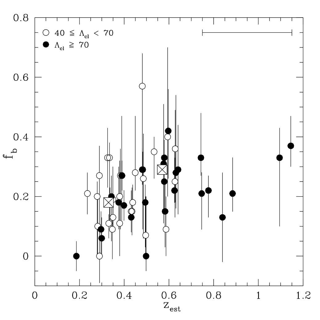
Figure 10: The fraction of blue galaxies ($f_{b}$) versus estimated redshift ($z_{est}$) for the 57 cluster candidates. In order to show all points, we have randomly offset the cluster $z_{est}$ by less than $\pm 0.05$. A richer subsample of clusters ($\Lambda_{cl}\geq 70$) is indicated by the filled circles. $f_{b}$ is only complete to $z_{est}\approx 0.6$. The errors in $f_{b}$ represent the range of possible values. The estimated redshift uncertainty is indicated in the upper right hand corner. The median values in the first two redshift bins are designated by the large boxed crosses. $f_{b}$ and $z_{est}$ are correlated at a 96.2% ($\sim 2\sigma$) confidence level (see §4).

The resulting background-subtracted $V_{4}$ – $I_{4}$ color distributions are examined. Following the BO analysis, we determine the ridge line of the early–type population for each cluster. We take the median color of each distribution as this characteristic color. The fraction of blue galaxies ($f_{b}$) for each cluster is then calculated relative to this color by using the corresponding $\Delta(V_{4}-I_{4})$ analytically determined above. The resulting $f_{b}$ of each cluster is listed in Table 1. Fig. 10 shows $f_{b}$ versus the estimated redshift ($z_{est}$). We indicate with different points a richer subset of clusters ($\Lambda_{cl}\geq 70$ in either the $V_{4}$ or $I_{4}$ band). The median values of the blue fraction (indicated by large boxed crosses in Fig. 10) are $f_{b}=\{0.18~{}0.29\}$ in the $0.2\leq z_{est}\leq 0.4$ and the $0.5\leq z_{est}\leq 0.7$ redshift intervals, respectively.

In order to estimate the error in $f_{b}$, we have calculated the standard error assuming Poissonian statistics; in addition, we have perturbed the background counts by $\pm 1\sigma$ and recalculated $f_{b}$. The uncertainty in $f_{b}$ represents the range of observed values for a particular cluster. We have not corrected the color distributions for the color–magnitude effect in E/S0 galaxies. This effect is the slight blueing of E/S0 galaxy colors as the galaxy absolute magnitude becomes fainter (Sandage & Visvanathan 1978). It broadens the color distribution of the early–type population and might, therefore, cause an artificial increase in $f_{b}$. We have tested this effect by recalculating $f_{b}$ with a color difference $\Delta(B-V)=0.4$. The resulting $f_{b}$ values are all within the lower error bars.

The scatter in $f_{b}$ is large, as is the uncertainty in the estimated redshift ($\sigma_{z_{est}}\mathrel{\hbox{\raise 2.15277pt\hbox{$<$}\hbox to0.0pt{\hss\lower 2.15277pt\hbox{$\sim$}}}}0.2$); however, if we take the data points strictly at face value, there is a correlation between the blue fraction $f_{b}$ and the estimated redshift $z_{est}$. We have quantified this by calculating the Spearman rank-order correlation coefficient for our data points. The correlation is significant at a 99.98% confidence level. In order to include the parameter uncertainties in this calculation, we have created 200 new datasets by randomly adding the appropriate error to each data point, assuming that the uncertainties in both parameters are gaussian. A correlation coefficient and significance level are then calculated for each new sample. The average significance of the correlation between $z_{est}$ and $f_{b}$ is 96.2% ($\sim 2\sigma$). The purpose of this statistical analysis is to show that there is a monotonic increase in the blue fraction with estimated redshift, not necessarily that there is a linear correlation between the two parameters as we have no reason to believe that the relationship is linear.

Our values of $f_{b}$ as a function of redshift are consistent with previous observations of intermediate and high–redshift clusters. We find blue fractions of $f_{b}\sim 0.05-0.2$ in clusters at $0.2\mathrel{\hbox{\raise 2.15277pt\hbox{$<$}\hbox to0.0pt{\hss\lower 2.15277pt\hbox{$\sim$}}}}z\mathrel{\hbox{\raise 2.15277pt\hbox{$<$}\hbox to0.0pt{\hss\lower 2.15277pt\hbox{$\sim$}}}}0.4$, consistent with the results of BO. By $z\sim 0.5$, $f_{b}$ reaches $\sim 0.3$. The trend in Fig. 10 suggests that, at redshifts of $z\mathrel{\hbox{\raise 2.15277pt\hbox{$>$}\hbox to0.0pt{\hss\lower 2.15277pt\hbox{$\sim$}}}}0.6$, the fraction of blue galaxies may be greater than 0.4. Rakos & Schombert (1995) find that the fraction of blue galaxies, as defined in the rest–frame Strömgren colors, is $f_{b}\sim 0.4-0.6$ at $z\sim 0.6$ and increases to values as high as 0.8 in clusters at $z=0.9$.

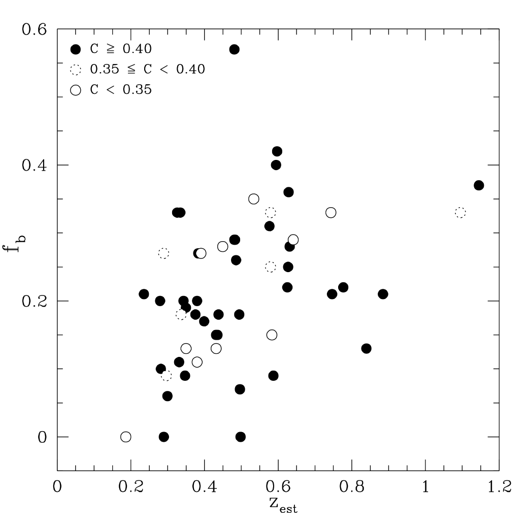
Figure 11: The fraction of blue galaxies ($f_{b}$) versus estimated redshift for the 57 cluster candidates. The symbols indicate three compactness ($C$) ranges of the cluster candidates (see §4). Filled circles, compact clusters ($C\geq 0.4$); open circles, open clusters ($C<0.35$); dotted circles, intermediate clusters ($0.35\leq C<0.4$).

BO found that the fraction of blue galaxies in open clusters increases with redshift at a rate similar to that in compact clusters, though $f_{b}$ was systematically larger (see §1). We have examined this relation in our data. Fig. 11 shows $f_{b}$ as a function of estimated redshift. We indicate with different symbols three ranges of the compactness parameter $C$ (defined above). Filled, dotted, and open circles indicate compact clusters ($C\geq 0.4$), intermediate clusters ($0.35\leq C<0.4$), and open clusters ($C<0.35$), respectively, as specified by BO. The typical PDCS clusters is compact (though not azimuthally symmetric; see Paper II). Considering the large uncertainty, there is no clear indication that the open or intermediate clusters have systematically higher blue fractions.

5 Summary

We have examined the color evolution of the galaxy populations of the richest candidate clusters of galaxies from the Palomar Distant Cluster Survey. The sample contains 57 intermediate and high–redshift clusters of galaxies, the largest statistical sample of distant clusters. Our principal conclusions are summarized below.

• For intermediate redshift ($z\mathrel{\hbox{\raise 2.15277pt\hbox{$<$}\hbox to0.0pt{\hss\lower 2.15277pt\hbox{$\sim$}}}}0.4$) clusters, we find that there is a distinct ridge line or “red envelope” in the color–magnitude diagram. The color of this locus corresponds well with the expected no–evolution color of present–day ellipticals at these redshifts. This result is consistent with previous optical studies of intermediate redshift clusters.

• At progressively higher redshifts, this red envelope, as characterized by the mean galaxy color, has shifted bluewards compared to the no–evolution prediction. By $z\sim 0.9$, there are only a few cluster galaxies which are as red in their rest–frame as present-day ellipticals. Through simple Monte–Carlo simulations of a synthetic non–evolving cluster population, we have confirmed that we are able to observe these very red members if they are present at these redshifts. The blueing trend of the mean galaxy color by $\sim 0.4$ mag at $z\sim 0.6$ and over 1 mag at $z\sim 0.8$ is consistent with that previously observed in the optical–infrared colors. A comparison between the observed color evolution in the Palomar clusters with simple Bruzual & Charlot (1996) models of passive aging of an old stellar population formed in a single burst of star formation indicates formation epochs of $z\mathrel{\hbox{\raise 2.15277pt\hbox{$>$}\hbox to0.0pt{\hss\lower 2.15277pt\hbox{$\sim$}}}}2$ for the early-type cluster galaxies.

• Though the uncertainties are large, the Butcher–Oemler effect is observed in the Palomar clusters. We find that the fraction of blue galaxies increases with the estimated redshift of the cluster at a 96.2% ($2\sigma$) confidence level. We observe blue fractions of $f_{b}\sim 0.05-0.2$ in clusters at redshifts of $0.2\mathrel{\hbox{\raise 2.15277pt\hbox{$<$}\hbox to0.0pt{\hss\lower 2.15277pt\hbox{$\sim$}}}}z\mathrel{\hbox{\raise 2.15277pt\hbox{$<$}\hbox to0.0pt{\hss\lower 2.15277pt\hbox{$\sim$}}}}0.4$. These fractions are consistent with that found previously by Butcher & Oemler (1984). Our calculations of $f_{b}$ are only complete to redshifts of $z\sim 0.6$; at these redshifts, $f_{b}\sim 0.3-0.4$. The observed trend indicates that clusters at $z\mathrel{\hbox{\raise 2.15277pt\hbox{$>$}\hbox to0.0pt{\hss\lower 2.15277pt\hbox{$\sim$}}}}0.6$ can have blue fractions which are greater than 0.4. This result is consistent with that found by Rakos & Schombert (1995). They have examined 17 clusters over a redshift range similar to ours and find that the blue fraction $f_{b}$ increases to 0.8 in clusters at $z\sim 0.9$.

The referee Jim Schombert is graciously thanked for his insightful comments and an extremely productive visit. It is also a pleasure to thank Marc Postman for his continual guidance and essential scientific contributions to this paper and Ian Smail for his special attention and thorough review of this text. Neta Bahcall, Jim Gunn, Michael Strauss, and Ed Turner are thanked for providing invaluable comments on a preliminary version. The following people are acknowledged for their generous contributions : Robert Lupton for his useful comments and aid in photometric conversions, Don Schneider for providing the spectral energy distributions and response functions, Stéphane Charlot and Ann Zabludoff for supplying and explaining the Bruzual & Charlot synthesis codes, and Stéphane Courteau for being available for scientific consultations. LML graciously acknowledges support from a Carnegie Fellowship and NASA contract NGT–51295.

Figure Captions

• The no-evolution $V_{4}-I_{4}$ color and the $V_{4}$ and $I_{4}$ band k-corrections as a function of redshift and morphological type as calculated using the spectral energy distributions from Coleman, Wu & Weedman (1980).

• Left : the expected color–magnitude relation for a simulated no–evolution cluster population as a function of redshift (see §3.1). The cluster redshift is indicated in the upper left corner of each panel. E/S0s are indicated by filled circles. Sab, Sbc, Scd, and Irr galaxies are indicated by circles, squares, triangles, and stars, respectively. The magnitude limits of the PDCS ($V_{4}^{ap}\approx 22.8$ and $I_{4}^{ap}\approx 21.4$) are indicated by solid lines. Right : the resulting color distributions. Solid line histograms represent the total color distribution, while shaded histograms represent the color distributions that would be observed in our survey.

• The expected composite color distributions in each of the three redshift intervals for the simulated no–evolution cluster populations (see §3.1). Solid line histograms represent the total color distribution, while shaded histograms represent the color distribution that would be observed in our survey. For clarity, the observed color distribution in the highest redshift interval is expanded in the small window in the bottom panel.

• Composite color–magnitude diagrams for each of the five PDCS fields. The aperture color, $(V_{4}-I_{4})_{ap}$, is plotted against the aperture $I_{4}$ magnitude, $I_{4}^{ap}$. The aperture magnitude limits have been applied. The top three panels show the composite CM diagrams for each of the three redshift intervals (see §3.2). Table 2 lists the number of cluster candidates in each panel. The bottom panels show the CM diagrams of regions of the five fields which contain no cluster galaxies (indicated as “field”).

• Composite color–magnitude diagrams of the Palomar clusters in each of the three redshift intervals. The aperture color, $(V_{4}-I_{4})_{ap}$, is plotted against the aperture $I_{4}$ magnitude, $I_{4}^{ap}$. The aperture magnitude limits have been applied. The bottom panel shows the CM diagram of sample regions of the five fields which contain no cluster galaxies (indicated as “field”).

• Composite aperture color distributions for each of the five PDCS fields. The cluster galaxy color distributions are shown before (solid line histograms) and after (shaded histograms) a statistical correction for the background. The aperture magnitude limits have been applied. The top three panels show the composite CM diagrams for each of the three redshift intervals (see §3.2). The bottom panels show the CM diagrams of regions of the five fields which contain no cluster galaxies (indicated as “field”).

• Composite aperture color distributions of the Palomar clusters in each of the three redshift intervals. Background has been subtracted. The redshift interval is listed in the upper left of each panel. The expected range of no–evolution E/S0s colors (Fig. 2) for each redshift interval is indicated by a bar (see §3.2).

• Comparison of the characteristic colors of the Palomar clusters for each of the three redshift bins (see §3) with the results of the Bruzual & Charlot models (see §3.3) : a $\tau=1~{}{\rm Gyr}$ burst of star formation (upper panel) and an exponentially decaying star formation rate with $\mu=0.5$ (lower panel). The lines represent different epochs of the initial star formation : $z_{f}=1$ (solid lines), $z_{f}=2$ (dotted lines), and $z_{f}=10$ (dashed lines) with $q_{o}=0$ (thin lines) and $q_{o}=0.5$ (thick lines). The vertical errors indicate the $1\sigma$ confidence limits on the characteristic color of the background-subtracted galaxy distribution (see §3.1). The horizontal errors indicate the approximate range of estimated redshifts in each bin.

• Composite aperture color distributions versus radial distance for a richer ($\Lambda_{cl}\geq 70$) sample of the PDCS clusters (see §3.4). Columns indicate each of the three redshift intervals. The radial range (in $h^{-1}~{}{\rm Mpc}$) around the cluster center is indicated in the upper left-hand corner of each panel.

• The fraction of blue galaxies ($f_{b}$) versus estimated redshift ($z_{est}$) for the 57 cluster candidates. In order to show all points, we have randomly offset the cluster $z_{est}$ by less than $\pm 0.05$. A richer subsample of clusters ($\Lambda_{cl}\geq 70$) is indicated by the filled circles. $f_{b}$ is only complete to $z_{est}\approx 0.6$. The errors in $f_{b}$ represent the range of possible values. The estimated redshift uncertainty is indicated in the upper right hand corner. The median values in the first two redshift bins are designated by the large boxed crosses. $f_{b}$ and $z_{est}$ are correlated at a 96.2% ($\sim 2\sigma$) confidence level (see §4).

• The fraction of blue galaxies ($f_{b}$) versus estimated redshift for the 57 cluster candidates. The symbols indicate three compactness ($C$) ranges of the cluster candidates (see §4). Filled circles, compact clusters ($C\geq 0.4$); open circles, open clusters ($C<0.35$); dotted circles, intermediate clusters ($0.35\leq C<0.4$).

Table 1 : Properties of the Sample of PDCS Clusters

Cluster	Redshift	Richness		Compactness	Blue Fraction
ID #	$z_{est}$	$\Lambda_{cl}$		$C$	$f_{b}$
001	0.6	61.5		$0.60^{+0.09}_{-0.09}$	$0.28^{+0.26}_{-0.12}$
002	0.4	52.1		$0.48^{+0.05}_{-0.05}$	$0.27^{+0.09}_{-0.18}$
003	0.6	88.5		$0.32^{+0.09}_{-0.02}$	$0.15^{+0.11}_{-0.12}$
004	0.6	94.9		$0.35^{+0.03}_{-0.02}$	$0.33^{+0.06}_{-0.12}$
006	0.5	62.9		$0.33^{+0.02}_{-0.02}$	$0.35^{+0.05}_{-0.09}$
008	0.6	75.3		$0.38^{+0.13}_{-0.11}$	$0.25^{+0.06}_{-0.09}$
009	0.4	58.1		$0.40^{+0.02}_{-0.02}$	$0.20^{+0.12}_{-0.20}$
010	0.3	58.8		$0.38^{+0.15}_{-0.11}$	$0.27^{+0.10}_{-0.18}$
011	0.4	104.5		$0.48^{+0.08}_{-0.09}$	$0.18^{+0.12}_{-0.09}$
012	0.3	75.5		$0.36^{+0.04}_{-0.06}$	$0.09^{+0.06}_{-0.09}$
014	0.4	46.4		$0.49^{+0.04}_{-0.06}$	$0.18^{+0.06}_{-0.05}$
015	1.1	78.5		$0.52^{+0.04}_{-0.05}$	$0.37^{+0.10}_{-0.07}$
016	0.5	108.6		$0.57^{+0.02}_{-0.02}$	$0.18^{+0.06}_{-0.15}$
017	0.7	115.0		$0.45^{+0.03}_{-0.02}$	$0.21^{+0.07}_{-0.12}$
018	0.4	54.0		$0.52^{+0.02}_{-0.02}$	$0.15^{+0.08}_{-0.08}$
019	0.6	66.3		$0.75^{+0.05}_{-0.23}$	$0.22^{+0.14}_{-0.04}$
020	0.4	50.2		$0.25^{+0.04}_{-0.04}$	$0.28^{+0.19}_{-0.06}$
021	0.3	45.2		$0.58^{+0.02}_{-0.02}$	$0.20^{+0.05}_{-0.20}$
022	0.4	64.7		$0.34^{+0.02}_{-0.02}$	$0.27^{+0.05}_{-0.05}$
023	0.2	44.6		$0.44^{+0.17}_{-0.14}$	$0.21^{+0.07}_{-0.07}$
024	0.4	66.8		$0.32^{+0.02}_{-0.05}$	$0.11^{+0.05}_{-0.07}$
025	0.3	49.5		$0.42^{+0.03}_{-0.02}$	$0.10^{+0.09}_{-0.10}$
030	0.3	46.5		$0.27^{+0.03}_{-0.02}$	$0.13^{+0.05}_{-0.05}$
031	1.1	120.0		$0.37^{+0.04}_{-0.07}$	$0.33^{+0.10}_{-0.23}$
033	0.5	42.5		$0.60^{+0.04}_{-0.18}$	$0.26^{+0.15}_{-0.20}$
034	0.3	62.0		$0.49^{+0.04}_{-0.04}$	$0.11^{+0.03}_{-0.05}$
035	0.6	67.5		$0.46^{+0.02}_{-0.02}$	$0.40^{+0.30}_{-0.20}$
036	0.3	54.7		$0.61^{+0.05}_{-0.11}$	$0.09^{+0.05}_{-0.10}$
037	0.6	60.0		$0.70^{+0.06}_{-0.17}$	$0.25^{+0.08}_{-0.12}$

Table 1 – Continued

Cluster	Redshift	Richness		Compactness	Blue Fraction
ID #	$z_{est}$	$\Lambda_{c}$		$C$	$f_{b}$
038	0.3	47.7		$0.61^{+0.02}_{-0.02}$	$0.33^{+0.05}_{-0.22}$
039	0.6	63.3		$0.72^{+0.04}_{-0.03}$	$0.09^{+0.11}_{-0.09}$
041	0.6	59.6		$0.63^{+0.07}_{-0.07}$	$0.36^{+0.13}_{-0.18}$
042	0.6	77.4		$0.61^{+0.27}_{-0.19}$	$0.31^{+0.20}_{-0.20}$
047	0.3	38.5		$--$	$--$
048	0.3	28.4		$0.47^{+0.04}_{-0.05}$	$0.20^{+0.07}_{-0.15}$
049	0.2	51.2		$--$	$--$
050	0.5	96.8		$0.46^{+0.08}_{-0.06}$	$0.29^{+0.07}_{-0.05}$
051	0.4	76.5		$0.51^{+0.05}_{-0.06}$	$0.17^{+0.05}_{-0.05}$
052	0.5	114.3		$0.71^{+0.02}_{-0.03}$	$0.29^{+0.06}_{-0.20}$
053	0.2	19.4		$0.32^{+0.02}_{-0.02}$	$0.00^{+0.05}_{-0.05}$
054	0.3	70.5		$0.51^{+0.03}_{-0.03}$	$0.06^{+0.07}_{-0.06}$
055	0.3	72.2		$0.37^{+0.02}_{-0.02}$	$0.18^{+0.05}_{-0.07}$
056	0.5	61.4		$0.47^{+0.04}_{-0.06}$	$0.00^{+0.20}_{-0.05}$
057	0.8	72.7		$0.64^{+0.06}_{-0.02}$	$0.22^{+0.05}_{-0.09}$
059	0.8	115.3		$0.57^{+0.14}_{-0.18}$	$0.13^{+0.15}_{-0.15}$
061	0.3	47.7		$0.57^{+0.04}_{-0.06}$	$0.19^{+0.11}_{-0.11}$
062	0.4	80.3		$0.32^{+0.02}_{-0.02}$	$0.13^{+0.05}_{-0.05}$
063	0.6	103.7		$0.32^{+0.02}_{-0.02}$	$0.29^{+0.15}_{-0.15}$
065	0.4	61.0		$0.43^{+0.22}_{-0.11}$	$0.15^{+0.07}_{-0.07}$
066	0.4	34.5		$0.56^{+0.14}_{-0.15}$	$0.27^{+0.20}_{-0.15}$
067	0.5	45.7		$0.40^{+0.04}_{-0.10}$	$0.57^{+0.11}_{-0.29}$
068	0.5	59.4		$0.40^{+0.02}_{-0.02}$	$0.07^{+0.13}_{-0.07}$
069	0.3	43.5		$0.42^{+0.02}_{-0.05}$	$0.00^{+0.09}_{-0.09}$
071	0.7	95.5		$0.32^{+0.14}_{-0.05}$	$0.33^{+0.15}_{-0.06}$
072	0.6	85.1		$0.40^{+0.07}_{-0.08}$	$0.42^{+0.14}_{-0.16}$
075	0.9	147.7		$0.54^{+0.03}_{-0.03}$	$0.21^{+0.12}_{-0.06}$
076	0.3	54.0		$0.43^{+0.02}_{-0.02}$	$0.33^{+0.10}_{-0.10}$

Table 2 : The Number of PDCS Clusters in Each Field

Redshift Interval	$00^{{\rm h}}$	$02^{{\rm h}}$	$09^{{\rm h}}$	$13^{{\rm h}}$	$16^{{\rm h}}$	total
$0.2\leq z_{est}\leq 0.4$	5	8	4	8	4	29
$0.5\leq z_{est}\leq 0.7$	5	3	6	5	4	23
$0.8\leq z_{est}\leq 1.2$	0	1	1	2	1	5

Table 3 : Statistical Descriptors of the $V_{4}-I_{4}$ Color Distribution of a Simulated Cluster Population

$z$	Total		Observed
	$C_{BI}$	$S_{BI}$	$C_{BI}$	$S_{BI}$
0.3	$1.19\pm 0.05$	$0.44\pm 0.03$	$1.20\pm 0.05$	$0.44\pm 0.03$
0.6	$2.10\pm 0.07$	$0.56\pm 0.04$	$2.20\pm 0.11$	$0.54\pm 0.07$
0.9	$2.60\pm 0.09$	$0.65\pm 0.06$	$2.40\pm 0.26$	$0.77\pm 0.16$

Table 4 : Statistical Descriptors of the Composite $V_{4}-I_{4}$ Color Distributions of Simulated Cluster Populations

Redshift Interval	Total		Observed
	$C_{BI}$	$S_{BI}$	$C_{BI}$	$S_{BI}$
$0.2\leq z\leq 0.4$	$1.19\pm 0.01$	$0.50\pm 0.02$	$1.20\pm 0.02$	$0.50\pm 0.02$
$0.5\leq z\leq 0.7$	$2.04\pm 0.02$	$0.60\pm 0.03$	$1.99\pm 0.03$	$0.59\pm 0.02$
$0.8\leq z\leq 1.2$	$2.58\pm 0.04$	$0.64\pm 0.03$	$2.44\pm 0.10$	$0.80\pm 0.05$

Table 5 : Statistical Descriptors of the Composite $V_{4}-I_{4}$ Color Distributions of the PDCS Clusters

Redshift Interval	$C_{BI}$	$S_{BI}$
$0.2\leq z_{est}\leq 0.4$	$1.34\pm 0.02$	$0.45\pm 0.05$
$0.5\leq z_{est}\leq 0.7$	$1.54\pm 0.06$	$0.54\pm 0.05$
$0.8\leq z_{est}\leq 1.2$	$1.21\pm 0.07$	$0.50\pm 0.09$

Table 6 : Statistical Descriptors of the Composite $V_{4}-I_{4}$ Color Distributions of the PDCS Clusters as a Function of Radius

Radial Interval	$0.2\leq z_{est}\leq 0.4$		$0.5\leq z_{est}\leq 0.7$		$0.8\leq z_{est}\leq 1.2$
$(h^{-1}~{}{\rm Mpc})$	$C_{BI}$	$S_{BI}$	$C_{BI}$	$S_{BI}$	$C_{BI}$	$S_{BI}$
$r\leq 0.25$	$1.34\pm 0.04$	$0.44\pm 0.03$	$1.60\pm 0.03$	$0.52\pm 0.04$	$1.27\pm 0.08$	$0.48\pm 0.08$
$0.25\leq r\leq 0.50$	$1.32\pm 0.05$	$0.45\pm 0.05$	$1.46\pm 0.04$	$0.55\pm 0.04$	$1.18\pm 0.07$	$0.52\pm 0.09$
$0.50\leq r\leq 0.75$	$1.41\pm 0.03$	$0.37\pm 0.06$	$1.36\pm 0.04$	$0.48\pm 0.04$	$1.31\pm 0.09$	$0.50\pm 0.07$

Figure 1: The no-evolution $V_{4}-I_{4}$ color and the $V_{4}$ and $I_{4}$ band k-corrections as a function of redshift and morphological type as calculated using the spectral energy distributions from Coleman, Wu & Weedman (1980).

Figure 2: Left : the expected color–magnitude relation for a simulated no–evolution cluster population as a function of redshift (see §3.1). The cluster redshift is indicated in the upper left corner of each panel. E/S0s are indicated by filled circles. Sab, Sbc, Scd, and Irr galaxies are indicated by circles, squares, triangles, and stars, respectively. The magnitude limits of the PDCS ($V_{4}^{ap}\approx 22.8$ and $I_{4}^{ap}\approx 21.4$) are indicated by solid lines. Right : the resulting color distributions. Solid line histograms represent the total color distribution, while shaded histograms represent the color distributions that would be observed in our survey.

Figure 3: The expected composite color distributions in each of the three redshift intervals for the simulated no–evolution cluster populations (see §3.1). Solid line histograms represent the total color distribution, while shaded histograms represent the color distribution that would be observed in our survey. For clarity, the observed color distribution in the highest redshift interval is expanded in the small window in the bottom panel.

Figure 4: Composite color-magnitude diagrams for each of the five PDCS fields. The aperture color, $(V_{4}-I_{4})_{ap}$, is plotted against the aperture $I_{4}$ magnitude, $I_{4}^{ap}$. The aperture magnitude limits have been applied. The top three panels show the composite CM diagrams for each of the three redshift intervals (see §3.2). Table 2 lists the number of cluster candidates in each panel. The bottom panels show the CM diagrams of regions of the five fields which contain no cluster galaxies (indicated as “field”).

Figure 5: Composite color–magnitude diagrams of the Palomar clusters in each of the three redshift intervals. The aperture color, $(V_{4}-I_{4})_{ap}$, is plotted against the aperture $I_{4}$ magnitude, $I_{4}^{ap}$. The aperture magnitude limits have been applied. The bottom panel shows the CM diagram of sample regions of the five fields which contain no cluster galaxies (indicated as “field”).

Figure 6: Composite aperture color distributions for each of the five PDCS fields. The cluster galaxy color distributions are shown before (solid line histograms) and after (shaded histograms) a statistical correction for the background. The aperture magnitude limits have been applied. The top three panels show the composite CM diagrams for each of the three redshift intervals (see §3.2). The bottom panels show the CM diagrams of regions of the five fields which contain no cluster galaxies (indicated as “field”).

Figure 7: Composite aperture color distributions of the Palomar clusters in each of the three redshift intervals. Background has been subtracted. The redshift interval is listed in the upper left of each panel. The expected range of no–evolution E/S0s colors (Fig. 2) for each redshift interval is indicated by a bar (see §3.2).

Figure 8: Comparison of the characteristic colors of the Palomar clusters for each of the three redshift bins (see §3) with the results of the Bruzual & Charlot models (see §3.3) : a $\tau=1~{}{\rm Gyr}$ burst of star formation (upper panel) and an exponentially decaying star formation rate with $\mu=0.5$ (lower panel). The lines represent different epochs of the initial star formation : $z_{f}=1$ (solid lines), $z_{f}=2$ (dotted lines), and $z_{f}=10$ (dashed lines) with $q_{o}=0$ (thin lines) and $q_{o}=0.5$ (thick lines). The vertical errors indicate the $1\sigma$ confidence limits on the characteristic color of the background-subtracted galaxy distribution (see §3.1). The horizontal errors indicate the approximate range of estimated redshifts in each bin.

Figure 9: Composite aperture color distributions versus radial distance for a richer ($\Lambda_{cl}\geq 70$) sample of the PDCS clusters (see §3.4). Columns indicate each of the three redshift intervals. The radial range (in $h^{-1}~{}{\rm Mpc}$) around the cluster center is indicated in the upper left-hand corner of each panel.

References

- (1) Abell, G.O. 1958, ApJS, 232, 689
- (2) Aragón-Salamanca, A., Ellis, R.S. & Sharples, R.M. 1991, MNRAS, 248, 128
- (3) Aragón-Salamanca, A., Ellis, R.S., Couch, W.J. & Carter, D. 1993, MNRAS, 262, 764 (A93)
- (4) Beers, T.C., Flynn, K. & Gebhardt, K. 1991, AJ, 100, 32
- (5) Bower, R.G., Lucey, J.A. & Ellis, R.S. 1992a, MNRAS, 254, 589
- (6) Bower, R.G., Lucey, J.A. & Ellis, R.S. 1992b, MNRAS, 254, 601
- (7) Butcher, H. & Oemler, A. 1978, ApJ, 226, 559
- (8) Butcher, H. & Oemler, A. 1984, ApJ, 285, 426 (BO)
- (9) Bruzual, A.G. 1983, ApJ, 273, 105
- (10) Bruzual, A.G. & Charlot, S. 1993, ApJ, 405, 538
- (11) Bruzual, A.G. & Charlot, S. 1996, ApJ, in preparation
- (12) Charlot, S. & Silk, J. 1994, ApJ, 432, 453
- (13) Coleman, G.D., Wu, C.C. & Weedman, D.W. 1980, ApJS, 43, 393
- (14) Couch, W.J. & Newell, E.B. 1984, ApJS, 56, 143
- (15) Couch, W.J., Ellis, R.S., Malin, D.F. & MacLaren, I. 1991, MNRAS, 249, 606
- (16) Couch, W.J., Ellis, R.S., Sharples, R.M. & Smail, I. 1994, ApJ, 430, 121
- (17) Dickinson, M. 1995, Fresh Views on Elliptical Galaxies, eds. A. Buzzoni et al., ASP Conference Series
- (18) Dressler, A. 1980, ApJ, 236, 351
- (19) Dressler, A. & Gunn, J.E. 1992, ApJS, 78, 1
- (20) Dressler, A., Oemler, A., Butcher, H.R. & Gunn, J.E. 1994, ApJ, 430, 107
- (21) Ellis, R.S., Couch, W.J., MacLaren, I. & Koo, D.C. 1985, MNRAS, 217, 239
- (22) Ellis, R.S., Smail, I., Dressler, A., Couch, W.J., Oemler, A., Butcher, H. & Sharples, R.M. 1996, ApJ, submitted
- (23) Frei, Z. & Gunn, J.E. 1994, AJ, 108, 1476
- (24) Fukugita, M., Shimasaku, K. & Ichikawa, T. 1995, PASP, 107, 945
- (25) Gunn, J.E., Hoessel, J. & Oke, J.B. 1986, ApJ, 306, 30
- (26) Gunn, J.E. & Dressler, A. 1988, in Towards Understanding Galaxies at Large Redshift, eds. R. Kron and A. Renzini, Dordrecht, p. 29
- (27) Jarvis, J.F. & Tyson, J.A. 1981, AJ, 86, 476
- (28) Landolt, A.U. 1992, AJ, 104, 340
- (29) Le Borgne, J.F., Pelló, R. & Sanahuja, B. 1992, A&AS, 95, 87
- (30) Lubin, L.M. 1995, PhD Thesis, Princeton University
- (31) Lubin, L.M. & Postman, M. 1996, AJ, in press (Paper II)
- (32) Lubin, L.M., Postman, M., Oke, J.B. & Gunn, J.E. 1996, in progress
- (33) Luppino, G.A., Cooke, B.A., McHardy, I.M. & Ricker, G.R. 1991, AJ, 102, 1
- (34) Millington, S.J.C. & Peach, J.V. 1990, MNRAS, 242, 112
- (35) Molinari, E., Banzi, M., Buzzoni, G., Chincarini, G. & Pedrana, M.D. 1994, A&AS, 103, 245
- (36) Oemler, A. 1974, ApJ, 914, 1
- (37) Oemler, A., Dressler, A. & Butcher, H. 1996, ApJ, submitted
- (38) Oke, J.B. & Gunn, J.E. 1983, ApJ, 266, 713
- (39) Oke, J.B., Gunn, J.E. & Hoessel, J.G. 1996, AJ, 111, 29
- (40) Pahre, M.A., Djorgovski, S.G. & de Carvalho, R.R. 1995, ApJ, 453, L17
- (41) Postman, M. & Geller, M.J. 1984, ApJ, 281, 95
- (42) Postman, M., Lubin, L.M., Gunn, J.E., Oke, J.B., Schneider, D.P., Hoessel, J.G. & Christensen, J.A. 1996, AJ, 111, 615 (Paper I)
- (43) Rakos, K.D. & Schombert, J.M. 1995, ApJ, 439, 47
- (44) Sandage, A. 1972, ApJ, 176, 21
- (45) Sandage, A. & Visvanathan, N. 1978, ApJ, 223, 707
- (46) Sandage, A., Bingelli, B. & Tammann, G.A. 1985, AJ, 90, 9
- (47) Scalo, J.M. 1986, Fundam. Cosmic Physics, 11, 1
- (48) Silva, D.R. & Elston, R. ApJ, 428, 511
- (49) Smail, I., Ellis, R.S. & Fitchett, M.J. 1994, MNRAS, 270, 245
- (50) Stanford, S.A., Eisenhardt, P.R.M. & Dickinson, M. 1995, ApJ, 450, 512
- (51) Steidel, C.C., Giavalisco, M., Pettini, M., Dickinson, M. & Adelberger, K.L. 1996, ApJ, in press
- (52) Valdes, F. 1982, Proc. SPIE, 313, 465
- (53) Visvanathan, N. & Sandage, A. 1977, ApJ, 216, 214
- (54) Zabludoff, A.I., Zaritsky, D., Lin, H., Tucker, D., Hashimoto, Y., Shectman, S.A., Oemler, A. & Kirshner, R.P. 1996, ApJ, submitted
- (55)