On cooling of magnetized neutron stars

Abstract

Cooling of neutron stars with dipole magnetic fields is simulated using a realistic model of the anisotropic surface temperature distribution produced by magnetic fields. Suppression of the electron thermal conductivity of outer stellar layers across the field increases thermal isolation of these layers near the magnetic equator. Enhancement of the radiative and longitudinal electron thermal conductivities in quantizing magnetic fields reduces thermal isolation near the magnetic poles. The equatorial increase of the isolation is pronounced for $B\;\raise 1.29167pt\hbox{$>$\kern-7.5pt\raise-4.73611pt\hbox{$\sim$}}\;10^{10}$ G, while the polar decrease – for $B\;\raise 1.29167pt\hbox{$>$\kern-7.5pt\raise-4.73611pt\hbox{$\sim$}}\;10^{12}$ G. The effects compensate partly each other, and the actual influence of the magnetic fields on the cooling is weaker than predicted by the traditional theories where the equatorial effects have been neglected.

1 Introduction

Thermal X-ray radiation has been observed recently with $ROSAT$ from at least four cooling neutron stars: PSR 0833-45, PSR 1055-52, PSR 0656+14 and Geminga (see, e.g., Ögelman 1995). A soft ($T_{\rm s}\sim(5$ – $10)\times 10^{5}$ K) component of the observed spectra is most probably emitted from all the visible neutron star (NS) surface. It pulses with the pulsar period, and the pulsed fraction, $\sim 10-30\%$, varies with photon energy. The spectra and the light curves of these middle-age ($10^{4}$ – $10^{6}$ yr) NSs contain important information on NS parameters and on the properties of superdense matter in NS interiors.

The pulsations are most probably caused by the temperature variation over the NS surface. The natural cause of the variation is non-uniformity of the surface magnetic field and anisotropy of the heat transport in strongly magnetized subphotospheric layers of cooling NSs (e.g., Yakovlev & Kaminker 1994).

So far most of the cooling calculations of NSs (e.g., Nomoto & Tsuruta 1987, Van Riper 1991) have been performed under the traditional simplified assumption that the magnetic field is radial everywhere over the stellar surface. In this case the thermal energy is carried through the subphotospheric layers along the magnetic field lines, and the surface temperature $T_{\rm s}$ is uniform and determined by the longitudinal (along the field $B$) thermal conductivity. The latter conductivity is mainly enhanced by the magnetic field, which increases $T_{\rm s}$ at given internal temperature $T_{\rm i}$. As a result, the traditional cooling theories predict (e.g., Van Riper 1991) that the strong magnetic fields $B\;\raise 1.29167pt\hbox{$>$\kern-7.5pt\raise-4.73611pt\hbox{$\sim$}}\;10^{12}$ G increase $T_{\rm s}$ (and the photon luminosity) at the neutrino cooling stage. At this stage, a NS is not too old (age $t\;\raise 1.29167pt\hbox{$<$\kern-7.5pt\raise-4.73611pt\hbox{$\sim$}}\;10^{4}$–$10^{5}$ yrs) and cools mainly via neutrino emission from the stellar interior. On the other hand, strong fields decrease $T_{\rm s}$ and accelerate the cooling at the subsequent photon cooling stage when the neutrino emission becomes low and the star cools via the thermal surface radiation.

The main disadvantage of the traditional approach is that it neglects those parts of the NS surface where $B$ is essentially non-radial, and the transverse thermal conductivity is important. The aim of this paper is to use a realistic model of heat transport and the related surface temperature distribution valid for any magnetic field geometry in the NS surface layers. The model generalizes the results of Greenstein & Hartke (1983), Van Riper (1989), Schaaf (1990a), and Page (1995) who performed detailed studies of the NS surface temperature either for restricted magnetic field geometries or under specified assumptions on thermal conductivity of stellar matter (see Sect. 2, for details). Adopting this model we will carry out the cooling calculations (Sect. 3). Our results show (Sects. 4 and 5) that the effects of the magnetic fields on the NS cooling are more sophisticated than anticipated previously.

2 Surface temperature distribution

Consider the temperature distribution over the surface of a magnetized NS. Let the star be not too young ($t\;\raise 1.29167pt\hbox{$>$\kern-7.5pt\raise-4.73611pt\hbox{$\sim$}}\;$ 1 – $10^{3}$ yrs), so that the internal thermal relaxation is achieved. Then the stellar interior is highly isothermal: $\tilde{T}=T(r)\exp(\Phi(r))$ is constant within the star, where $T(r)$ is the local internal temperature, $r$ is radial coordinate, $\Phi(r)$ is the gravitational redshift function which takes into account the effects of General Relativity (e.g., Glen & Sutherland 1980). The isothermal interior is surrounded by a very thin subphotospheric layer. Its thickness ( $<$$\sim$  several meters) is much smaller than the stellar radius $R\sim 10$ km. This layer produces the thermal isolation of the NS interior. The temperature at the bottom of this layer is $T_{\rm i}=\tilde{T}\exp(-\Phi_{s})$, where $\Phi_{s}\approx\Phi(R)=0.5\ln(1-R_{g}/R)$, $R_{g}=2GM/c^{2}$ is the gravitational stellar radius, and $M$ is the stellar mass. While the star cools down, the isolating layer becomes thinner (e.g., Gudmundsson et al. 1983, Yakovlev & Kaminker 1994). The layer consists of two sublayers. In the inner one, the electrons are degenerate, and they are the main heat carriers. In the outer sublayer, the electrons are non-degenerate, and heat is mostly transported by radiation. In a rather cold NS, the surface layer may become solid, and the non-degenerate sublayer disappears.

The effective surface temperature $T_{\rm s}$ is determined by the heat transport through the isolating magnetized layer. The problem of calculating $T_{\rm s}$ is complicated (Yakovlev & Kaminker 1994), and the exact solution has not yet been found. Let us discuss a realistic model solution. Since the isolating layer is thin it is reasonable to adopt a plane-parallel one-dimensional approximation almost everywhere over the surface. We assume that the magnetic field is constant in each local part of the surface layer. Let the thermal flux $F$ be normal (radial) to the surface and the tangential flux be insignificant. Then $F=\sigma T_{\rm s}^{4}$, where $T_{\rm s}$ is the local effective surface temperature, and $\sigma$ is the Stefan – Boltzmann constant. It is well known that $T_{\rm s}$ depends on the internal temperature $T_{\rm i}$, and on the surface gravity $g_{\rm s}=(GM/R^{2})/\sqrt{(}1-R_{g}/R)$ ($T_{\rm s}\propto g_{\rm s}^{1/4}$; see, e.g., Gudmundsson et al. 1983). In our case, the local surface temperature $T_{\rm s}=T_{\rm s}(B,\chi)$ depends also on the local magnetic field $B$ and on the angle $\chi$ between $B$ and the normal to the surface. If $T_{\rm s}(B,\chi)$ is known, the NS total thermal luminosity is given by

$$L(T_{\rm i})=\sigma R^{2}\,\int T_{\rm s}^{4}(B,\chi)\,\mbox{d}\Omega$$ (1)

($\mbox{d}\Omega$ being solid angle of a surface element), and the redshifted luminosity (for distant observers) is $L^{\infty}=L(1-R_{g}/R)$.

Let the thermal energy in the isolating layer be carried by the thermal conduction (no convection or turbulent motion). Then the thermal balance yields

$$(\kappa_{\parallel}\cos^{2}\chi+\kappa_{\perp}\sin^{2}\chi)\;{\mbox{d}T\over\mbox{d}z}=F,$$ (2)

where $\kappa_{\parallel}$ and $\kappa_{\perp}$ are, respectively, the longitudinal and transverse (with respect to $B$) thermal conductivities, and $z$ is depth from the surface within the star in the locally flat reference frame. The equation of thermal balance should be supplemented by the equation of hydrostatic equilibrium; we assume (as in all cooling theories) that the magnetic field in the NS surface layers is force-free. Both equations should be integrated from the surface inside the star yielding the temperature and density profiles in the outer NS layer with given flux $F$ (i.e., with given $T_{\rm s}$). With increasing $z$, the temperature $T(z)$ tends to a constant value to be defined as the internal temperature $T_{\rm i}$. Combining the solutions for different $T_{\rm s}$, $B$ and $\chi$ one can determine the dependence of the effective local surface temperature $T_{\rm s}$ on $T_{\rm i}$, $B$ and $\chi$.

Since the thermal conductivities $\kappa_{\parallel}$ and $\kappa_{\perp}$ depend generally on $T$, $B$ and density $\rho$ the solution is complicated even with the above simplifications. Instead, we shall use the following model solution (Greenstein & Hartke 1983)

$$T_{\rm s}^{4}(B,\chi)=T_{\parallel}^{4}(B)\cos^{2}\chi+T_{\perp}^{4}(B)\sin^{2}\chi,$$ (3)

where $T_{\parallel}(B)=T_{\rm s}(B,0)$ is the surface temperature for the case when $B$ is normal to the surface (at the magnetic pole), and $T_{\perp}(B)=T_{\rm s}(B,\pi/2)$ is the same for the case when $B$ is tangential to the surface (at the magnetic equator).

Let us discuss briefly the properties of Eq. (3). First, (3) yields exact solution of the thermal conduction problem (2) for $B$ normal or tangential to the NS surface. Second, (3) reproduces the limit of $B=0$. Third, one can easily prove that (3) provides the solution for the case when $\kappa_{\parallel}\gg\kappa_{\perp}$. The case is realized for not very weak magnetic fields and not too close to the magnetic equator ($\kappa_{\parallel}\cos^{2}\chi\gg\kappa_{\perp}\sin^{2}\chi$). This case is very important since the transverse electron conductivity of degenerate electrons is much smaller than the longitudinal one, typically, at $B\;\raise 1.29167pt\hbox{$>$\kern-7.5pt\raise-4.73611pt\hbox{$\sim$}}\;10^{10}$ G (e.g., Yakovlev & Kaminker 1994). Fourth, Eq. (3) is exact for the case when $\kappa_{\perp}/\kappa_{\parallel}$ is constant (independent of depth $z$) for a given local part of the NS surface layer. The latter case is also important. For instance, it is realized in a strongly degenerate non-relativistic electron gas at not too high fields $B$ if the electron conductivity is produced by Coulomb scattering on atomic nuclei and the nuclei constitute a gas or liquid (e.g., Yakovlev & Kaminker 1994). The model solution (3) can actually be inaccurate at high magnetic fields near the magnetic equator where the thermal flux tangential to the surface can be substantial and the plane-parallel approximation can fail. However these areas of the NS surface give small contribution into the total stellar luminosity (1), and, thus, they seem to be insignificant for cooling simulations.

Using Eq. (2) one can obtain the following inequality of the thermal conduction problem

$$T_{\rm s}(B,\chi)\geq T_{\parallel}(B)\sqrt{\cos\chi}.$$ (4)

This inequality gives the lower limit to the effective surface temperature as a function of $\chi$. It follows from Eq. (2) by keeping the most important longitudinal thermal conductivity but neglecting the transverse conductivity (which is often much lower). In this case the surface temperature $T_{\rm s}(B,\chi)$ is naturally expressed through $T_{\parallel}(B)$. If $\kappa_{\parallel}\gg\kappa_{\perp}$ and $\kappa_{\parallel}\cos^{2}\chi\gg\kappa_{\perp}\sin^{2}\chi$ one can expect the real surface temperature to be very close to the lower limit. The inequality (3) can be useful for testing numerical calculations of $T_{\rm s}$ in magnetized NSs.

Equation (3) was first obtained by Greenstein & Hartke (1983). The authors derived (3) as an estimate assuming actually that the thermal conductivities $\kappa_{\parallel}$ and $\kappa_{\perp}$ are constant in the isolating layer. We emphasize that the equation is valid under much wider assumptions. Recently the solution similar to (3) has been proposed by Page (1995) for a dipole magnetic field. However, he used $T_{\rm s}(B_{\rm p},0)$ instead of $T_{\parallel}(B)$, and $T_{\rm s}(B_{\rm eq},\pi/2)$ instead of $T_{\perp}(B)$ on the right-hand side ($B_{\rm p}$ and $B_{\rm eq}$ being the polar and equatorial magnetic fields, respectively). The actual difference of his formula from Eq. (3) is not large but Eq. (3) is thought to be more adequate.

The advantage of Eq. (3) is that it reduces the calculation of $T_{\rm s}(B,\chi$) to solving two heat conduction problems: for $B$ normal ($T_{\parallel}(B)$) and tangential ($T_{\perp}(B)$) to the surface, as if at the magnetic pole and equator, respectively. The longitudinal (polar) problem has been considered very thoroughly by Van Riper (1989), and we use his results. We have taken the dependence of $T_{\rm s}$ on $T_{\rm i}$ from his Fig. 29 for $B$= 0, $10^{11}$, $10^{11.5}$, $10^{12}$, $10^{12.5}$, $10^{13}$, $10^{13.5}$ G and for the surface gravity $g_{\rm s}=10^{14}$ cm s^-2. We have interpolated these data for intermediate values of $B$. The transverse (equatorial) heat transfer problem has been analyzed by Schaaf (1991a). We have taken the dependence of $T_{\rm s}$ on $T_{\rm i}$ from his fitting Eqs. (29) and Table 3 for $B$= $10^{11}$, $10^{12}$, and $10^{13}$ G at $g_{\rm s}=10^{14}$ cm s^-2. We have interpolated these data for intermediate values of $B$, and extrapolated them to lower $B$ (if required) in such a way to reproduce the $B=0$ dependence of Van Riper (1989). We have used the scaling relation $T_{\rm s}\propto g_{\rm s}^{1/4}$ to extend the results to the surface gravities of study (Sect. 3).

Equation (3) is valid for any magnetic field geometry. For simplicity, we assume that the surface magnetic field is dipolar. Let $B_{\rm p}$ be the polar magnetic field, and let us introduce the reference frame which is flat for a local part of the NS subphotospheric layer. Taking into account the effects of General Relativity on the dipole field configuration (Ginzburg & Ozernoy 1964) one has

$$B_{R} = B_{\rm p}\,\cos\Theta,\;\;\;B_{\Theta}=-B_{\rm p}\,f\,\sin\Theta,$$ (5)

$$f = {(1-u)\ln(1-u)+u-0.5u^{2}\over\ln(1-u)+u+0.5u^{2}},$$

where $B_{R}$ and $B_{\Theta}$ are, respectively, the radial and tangential field components, $\Theta$ is the colatitude (with $\Theta=0$ at the pole), and $u=R_{g}/R$. If $u\ll 1$ the General Relativity effects are negligible and $f=-1/2$. With increasing $u$, the General Relativity effects make the field more radial.

Figure 1 shows the surface temperature distributions for a NS with $M=1.3\,M_{\odot}$ and $R=11.70$ km for two internal temperatures: $T_{\rm i}=10^{8}$ and $10^{7}$ K, typical for the neutrino and photon cooling stages, respectively, see Sects. 3 and 4 below. The results can be explained as follows.

Figure 1: Distribution of the effective temperature $T_{\rm s}$ from the pole (colatitude=0) to the equator (90) of the 1.3 $M_{\odot}$ neutron star with the dipole magnetic field for two values of the internal temperature ($T_{\rm i}$ = 10⁷ and 10⁸ K) and several polar field strengths $B_{\rm p}$. Open circles show the lower $T_{\rm s}$ limit, Eq. (4), for $B_{\rm p}=10^{12}$ G and $T_{\rm i}$ = 10⁷ K. Thin long dashes — $T_{\rm s}$ for the same dipolar field calculated without General Relativity effects ($f=-1/2$ in Eq. (5)).

The magnetic fields affect the heat transfer in two ways (e.g., Yakovlev & Kaminker 1994). First, the fields $B\;\raise 1.29167pt\hbox{$>$\kern-7.5pt\raise-4.73611pt\hbox{$\sim$}}\;10^{10}$ G magnetize the electrons in the degenerate sublayer of the outer isolating layer (see above). Rapid electron Larmor rotation ($\omega_{B}\tau\;\raise 1.29167pt\hbox{$>$\kern-7.5pt\raise-4.73611pt\hbox{$\sim$}}\;1$, where $\omega_{B}$ is the gyrofrequency of electrons at the Fermi surface, and $\tau$ is the electron relaxation time) suppresses the transverse conductivity making the thermal conduction anisotropic. Second, the fields $B\;\raise 1.29167pt\hbox{$>$\kern-7.5pt\raise-4.73611pt\hbox{$\sim$}}\;10^{12}$ G quantize electron motion – the structure of the electron Landau levels become pronounced in the thermodynamic and kinetic properties of degenerate and non-degenerate electrons.

As seen from Fig. 1, the field $B_{\rm p}\leq 10^{10}$ G is too low to modify noticeably the surface temperature $T_{\rm s}$ – the temperature is nearly isotropic over the surface. The magnetic fields $10^{10}\;\raise 1.29167pt\hbox{$<$\kern-7.5pt\raise-4.73611pt\hbox{$\sim$}}\;B\;\raise 1.29167pt\hbox{$<$\kern-7.5pt\raise-4.73611pt\hbox{$\sim$}}\;10^{12}$ G magnetize but not quantize the electron motion. They strongly reduce the transverse thermal conductivity of degenerate electrons enhancing thermal isolation of the NS. These fields do not affect significantly the longitudinal electron conductivity, the radiative thermal conductivity of outer non-degenerate sublayers, and thermodynamic properties of matter. Accordingly the polar surface temperature $T_{\parallel}$ remains nearly the same as for $B=0$ but the equatorial temperature $T_{\perp}$ can be noticeably reduced. With increasing $B$, the reduction becomes stronger, and $T_{\rm s}(B,\chi)$ approaches the minimum value $T_{\parallel}(B)\sqrt{\cos\chi}$ given by (4) almost everywhere at the surface except very near to the equator. As a result, the total luminosity (1) decreases with growing $B$ but this decrease saturates after the inequality $\kappa_{\parallel}\gg\kappa_{\perp}$ is achieved.

The quantizing magnetic fields $B\;\raise 1.29167pt\hbox{$>$\kern-7.5pt\raise-4.73611pt\hbox{$\sim$}}\;10^{12}$ G induce strong quantum oscillations of the thermal conductivity of degenerate electrons. Generally, these fields increase the longitudinal electron conductivity. They also increase the longitudinal and transverse radiative thermal conductivity of non-degenerate layers. Moreover, the strongly quantizing fields reduce the pressure of degenerate electrons. All these effects lower the thermal isolation. Accordingly, they increase the polar surface temperature while the equatorial surface temperature remains strongly damped by the magnetization of degenerate electrons (Fig. 1, curves with $B_{\rm p}=10^{13}$ G). The net effect is to enhance the total thermal luminosity $L$ of the star. With increasing $B$, the effect does not saturate but becomes more pronounced. The effects of the magnetic fields are stronger for a colder NS, where the isolating layer is thinner and more sensitive to the magnetic fields (e.g., Kaminker & Yakovlev 1994).

Therefore the thermal luminosity is suppressed by the magnetizing fields in the equatorial region and enhanced by the quantizing fields in the polar region. Two effects, the suppression and the enhancement, act in different ranges of $B$ and in opposite directions. The traditional calculations of NS cooling assume that the magnetic field is radial (polar) everywhere over the surface. Accordingly the calculations take into account the enhancement but neglect the suppression. The model surface temperature distribution (3) allows one to include both effects at once.

The validity of Eq. (3) can be checked by direct 2D simulations of the heat transport problem in the surface layers of a magnetized NS. The first attempt to perform 2D simulations was made by Schaaf (1991b) under many simplified assumptions. Nevertheless, the 2D effects such as the heat flow from the hotter polar regions to the cooler equatorial ones produced by heat conduction or/and meridional and convective motions should only smooth the temperature variations over the NS surface. In this respect $T_{\rm s}$ given by (3) can be considered as an upper limit of the possible temperature variation over the NS surface. It seems sufficient for our cooling calculations.

3 Cooling calculations

In order to analyze the effects of the magnetic fields on the NS cooling we have performed a series of numerical simulations. We have used the cooling code of Gnedin & Yakovlev (1993) and Gnedin et al. (1994) based on the approximation of isothermal NS interior. The cooling consists of two stages: the neutrino and photon ones. At the initial neutrino stage ($t\;\raise 1.29167pt\hbox{$<$\kern-7.5pt\raise-4.73611pt\hbox{$\sim$}}\;(10^{5}$ – $10^{6})$ yrs) the NS cools mainly due to the emission of neutrinos from its interior. The internal temperature is ruled by the neutrino luminosity, and it is independent of the surface temperature; the surface thermal radiation just follows the internal cooling. At the later photon stage the star becomes colder, and the neutrino production mechanisms are inefficient. The star cools mainly via thermal surface radiation which governs the fall of the internal temperature.

In our simulations, the equation of state of matter in the NS core has been taken from Prakash et al. (1988). According to this equation of state, the core consists of neutrons, protons and electrons (no hyperons or exotic particles). The maximum mass of a stable NS is 1.7 $M_{\odot}$. We have chosen two representative models, with $M$=1.3 $M_{\odot}$ and 1.44 $M_{\odot}$.

The model $M$=1.3 $M_{\odot}$ ($R$=11.70 km, the central density $\rho_{c}=1.12\times 10^{15}$ g cm^-3) is typical for a NS with the standard neutrino energy losses. In the cores of such stars, neutrinos are produced by the modified Urca processes and the nucleon-nucleon neutrino-pair bremsstrahlung (Friman & Maxwell 1979, Yakovlev & Levenfish 1995). The modified Urca reactions are $n+N\rightarrow p+e+N+\bar{\nu}_{e}$, $p+e+N\rightarrow n+N+\nu_{e}$, where $N$ is a spectacular nucleon required to satisfy momentum conservation. Until recently, it has been widely assumed that the main contribution into the modified Urca comes from the neutron branch reaction ($N=n$). However according to Yakovlev & Levenfish (1995) the proton branch reaction ($N=p$) is of comparable efficiency, and we have included it into the calculation. The nucleon-nucleon bremsstrahlung ($N+N\rightarrow N+N+\nu+\bar{\nu}$) consists of three branches ($n+n$, $n+p$, $p+p$), and all of them have been incorporated using the results of Friman & Maxwell (1979) and Yakovlev & Levenfish (1995). The effective masses of neutrons and protons (which enter the expressions for the neutrino energy loss rates and heat capacities) have been set equal to 0.7 of the bare masses.

Figure 2: Photon thermal luminosity $L^{\infty}$ (redshifted for distant observers) versus age of the 1.3 $M_{\odot}$ neutron star (the standard cooling) with a dipole magnetic field for several polar field strengths $B_{\rm p}$.

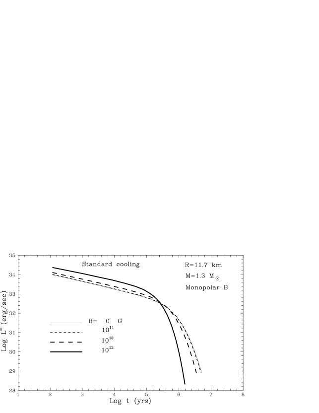
Figure 3: Same as for Fig. 2 but for radial (monopolar) magnetic fields of several strengths $B$.

The model $M$=1.44 $M_{\odot}$ ($R$=11.37 km, $\rho_{c}=1.37\times 10^{15}$ g cm^-3) represents a massive NS whose neutrino luminosity is greatly enhanced (Lattimer et al. 1991) by the direct Urca process ($n\rightarrow p+e+\bar{\nu}_{e}$, $p+e\rightarrow n+\nu_{e}$). The latter process intensifies the neutrino energy production rate by about 5 orders of magnitude for $T_{\rm i}\sim 10^{9}$ K. The direct Urca is a threshold reaction: it is allowed (Lattimer et al. 1991) for certain equations of state at rather high densities (to satisfy momentum conservation of the reacting particles). For the given equation of state, the critical threshold density is $\rho_{cr}=1.30\times 10^{15}$ g cm^-3. In our NS model, the direct Urca is allowed in a small central kernel of the star with $\rho>\rho_{c}$; the kernel radius is 2.32 km and its mass is 0.035 $M_{\odot}$. The neutrino luminosity of the kernel greatly exceeds the neutrino luminosity from all other parts of the star.

In both NS models we have also taken into account the neutrino luminosity of the stellar crust produced by neutrino-pair bremsstrahlung of electrons colliding with atomic nuclei. This has been done in the same simplified manner as in the work of Maxwell (1979). We have neglected the contribution of the crust into the NS heat capacity, since the crust mass is very low in our models. The mass of the crust in a NS with stiff equation of state and/or in a low-mass NS can be larger, i.e., in principle, the crust can contribute noticeably into the heat capacity. In our models, the heat capacity is produced by neutrons, protons and electrons in the NS core. We neglect possible superfluidity of neutrons and protons since our main goal is to study the influence of the surface magnetic fields on NS cooling. The latter influence is determined by isolating properties of the NS surface layers (Sect. 2), and it is not connected directly with the internal superfluidity.

We have adopted the dipole magnetic field geometry, Eq. (5), as described in Sec. 2. Using Eqs. (3) and (5) we can easily calculate the photon thermal NS luminosity which is an important ingredient of the cooling code. We have checked that the General Relativity effects in the magnetic field distribution (5) are almost negligible (Fig. 1) for our NS models. For comparison, we have also considered the case when the magnetic field is radial and has the same strength everywhere over the NS surface. This monopolar field geometry is traditional for the NS cooling theories. The field strengths have been varied from $B=0$ to $B\sim 10^{13}$ G. We have followed the cooling until the mean effective surface temperature drops below $10^{5}$ K. It has been unreasonable to proceed further since the results of Van Riper (1989) and Schaaf (1991a) used for calculating $T_{\rm s}$ are obtained for a not too cold NS.

4 Results and discussion

Figures 2 and 3 show the standard ($1.3\,M_{\odot}$) cooling curves for the dipolar and monopolar magnetic fields of different strengths. The curves display redshifted NS photon luminosity versus age $t$. Since the surface temperature is distributed nonuniformly, the NS radiation, as detected by a distant observer, depends on angle between line of sight and the magnetic axis. We present the luminosity from the total NS surface which is important for NS cooling theories but does not necessarily determine the radiation flux in a specific direction. The field geometry is seen to be very important. The monopolar magnetic field always reduces the NS thermal isolation (only the electron quantization effects operate). Accordingly, the monopolar field increases the photon luminosity $L$ at the neutrino cooling stage ($t\;\raise 1.29167pt\hbox{$<$\kern-7.5pt\raise-4.73611pt\hbox{$\sim$}}\;3\times 10^{5}$) K, and decreases $L$ at the subsequent photon cooling stage. This is typical for the traditional cooling calculations (e.g., Van Riper 1991). On the contrary, the dipolar field $B_{\rm p}=10^{11}$ G, for example, decreases $L$ at the neutrino cooling stage, and increases at the photon stage. This is certainly because the magnetizing fields enhance the equatorial thermal isolation. However, for larger $B_{\rm p}$, the polar drop of the thermal isolation becomes more important and produces just the traditional cooling effect: it raises $L$ at the neutrino cooling stage and decreases at the photon stage. With increasing $B_{\rm p}$, the polar effect becomes stronger than the equatorial one, but both effects interfere, and the results are quantitatively different from the traditional ones.

Figure 4: Ratio $L(B)/L(0)$ of the photon luminosities of magnetized and non-magnetized 1.3 $M_{\odot}$ neutron stars with dipolar (Fig. 2) and monopolar (Fig. 3) fields versus field strengths for several stellar ages $t$[yrs] (values of $\lg(t)$ are given near the curves)

The above effects are also illustrated in Fig. 4 where we plot $L(B)/L(0)$ versus $B$ for the $1.3\,M_{\odot}$ NS of several ages. For the monopolar field, the dependence of $L(B)/L(0)$ on $B$ at given age is monotonic, and one needs $B\;\raise 1.29167pt\hbox{$>$\kern-7.5pt\raise-4.73611pt\hbox{$\sim$}}\;10^{12}$ G to affect the cooling. For the dipolar field, the same dependence is non-monotonic, and the fields $B\;\raise 1.29167pt\hbox{$>$\kern-7.5pt\raise-4.73611pt\hbox{$\sim$}}\;10^{10}$ G affect noticeably the cooling curves. It is remarkable that the dipolar fields $B_{\rm p}\approx 3\times 10^{12}$ almost do not affect the NS cooling. For these fields, the enhancement of the equatorial isolation nearly compensates the drop of the polar one, and the cooling proceeds just as if the NS were non-magnetized. Nevertheless the field $B_{\rm p}\approx 3\times 10^{12}$ makes the surface temperature distribution very anisotropic (Fig. 1), which can produce strong modulation of the surface thermal radiation (Shibanov et al. 1995). When $B_{\rm p}\;\raise 1.29167pt\hbox{$<$\kern-7.5pt\raise-4.73611pt\hbox{$\sim$}}\;3\times 10^{12}$ G, the equatorial effects prevail while for $B_{\rm p}\;\raise 1.29167pt\hbox{$>$\kern-7.5pt\raise-4.73611pt\hbox{$\sim$}}\;3\times 10^{12}$ G the traditional polar effects are stronger. Note that strong dependence of $L(B)/L(0)$ on $B$ for $\lg(t[yr])=$ 6 and 6.3 is partially explained by steep slopes of the cooling curves (Fig. 2) at the photon cooling stage. Figures 5 and 6 plot the cooling curves for the $1.44\,M_{\odot}$ NS. The curves for this (rapidly cooling) NS are qualitatively the same as for the standard cooling (Figs. 2 and 3). However the photon luminosity $L$ is much lower than for the standard cooling since the rapid cooling goes much faster at the neutrino cooling stage. The appropriate luminosity ratios $L(B)/L(0)$ versus $B$ for several stellar ages are shown in Fig. 7. The curves are quite similar to those for the standard cooling (Fig. 4).

Figure 5: Same as in Fig. 2 for the 1.44 $M_{\odot}$ neutron star (rapid cooling).

Figure 6: Same as in Fig. 3 for the 1.44 $M_{\odot}$ neutron star.

5 Conclusions

We have used a realistic model (3) of the anisotropic distribution of the effective temperature $T_{\rm s}$ over the surface of a magnetized NS and have calculated NS cooling. We have considered both standard and rapid cooling of the NS with the dipole magnetic field. The results are noticeably different from the traditional results obtained for radial (monopolar) magnetic fields. We have shown (Figs. 2–7) that the dipole fields $10^{10}\;\raise 1.29167pt\hbox{$<$\kern-7.5pt\raise-4.73611pt\hbox{$\sim$}}\;B_{\rm p}\;\raise 1.29167pt\hbox{$<$\kern-7.5pt\raise-4.73611pt\hbox{$\sim$}}\;3\times 10^{12}$ G decrease the stellar photon luminosity at the neutrino cooling stage (by a factor of $\sim 2$), and increase the luminosity at the photon cooling stage (by about one order of magnitude), as compared to a non-magnetized NS, contrary to the traditional theories developed for monopolar magnetic fields. The effect is produced by the growth of the thermal isolation of the equatorial surface layers due to the low thermal conductivity of degenerate electrons across the magnetic field. On the other hand, the dipole fields $B_{\rm p}\;\raise 1.29167pt\hbox{$>$\kern-7.5pt\raise-4.73611pt\hbox{$\sim$}}\;3\times 10^{12}$ G increase the photon thermal luminosity at the neutrino cooling stage and decrease the luminosity at the photon cooling stage, in comparison with the luminosity at $B=0$. This conclusion agrees qualitatively with the results of the traditional theories but the actual magnetic field effect is much weaker than predicted by these theories due to the interference with the opposite effect in the equatorial regions. We have obtained also that the dipole field with $B_{\rm p}\approx 3\times 10^{12}$ G has almost no effect on the NS cooling.

Our results are based on a model of the surface temperature distribution applied to the dipole magnetic field. It would be easy to consider the NS cooling for other magnetic field geometries (quadrupole, shifted dipole, etc.), and the results are expected to be qualitatively the same as for the dipole field: the parts of the surface with essentially non-radial magnetic fields should noticeably increase the thermal isolation (Sect. 2).

For further studies of the magnetic field effects on the NS cooling, it would be highly desirable to perform detailed investigation of the heat transport in the outer NS layers using the best microscopic physics available (equation of state, thermal conductivities, etc), and obtain thus exact surface temperature distribution in magnetized NSs. The distribution (3) used above is expected to give an upper limit for the surface temperature variation produced by the magnetic fields (Sect. 2). It can be used for a test in more advanced theories. Even if (3) is not very accurate at large magnetic fields near the equatorial regions, it can yield quite accurate results since the cold equatorial surface parts do not contribute significantly into the photon luminosity (1).

Figure 7: Same as in Fig. 4 for the 1.44 $M_{\odot}$ neutron star.

The results of this work can be useful for theoretical interpretation of thermal X-ray radiation of NSs. All the objects from which this radiation has been detected (Sect. 1) are thought to possess magnetic fields of about several times of $10^{12}$ G. We can expect that such fields do not affect significantly the NS cooling but they can produce strongly anisotropic surface temperature variation and associated modulation of the surface thermal radiation.

The magnetic fields broaden the allowed ranges of the photon luminosities in the $L$–$t$ diagram for NSs of various masses, radii and equations of state with standard or enhanced neutrino energy losses (e.g., Ögelman 1994). According to the traditional theories, high magnetic fields increase the upper boundary of the expected photon luminosity at the neutrino cooling stage (typically, at $10^{2}\;\raise 1.29167pt\hbox{$<$\kern-7.5pt\raise-4.73611pt\hbox{$\sim$}}\;t\;\raise 1.29167pt\hbox{$<$\kern-7.5pt\raise-4.73611pt\hbox{$\sim$}}\;3\times 10^{5}$ yrs) and decrease the lower boundary of $L$ at the photon stage. Our results (Figs. 4 and 7) show that the dipolar fields $B\sim 10^{11}$ G decrease the lower boundary of $L$ at the neutrino stage and increase the upper boundary at the photon stage.

- [1] Ginzburg V.L. & Ozernoy L.M. 1964. Zh. Eksper. Teor. Fiz. 47, 1030
- [2] Glen G. & Sutherland P. 1980, ApJ, 239, 671
- [3] Gnedin O.Y. & Yakovlev D.G. 1993, Astron. Lett., 19, 104
- [4] Gnedin O.Y., Yakovlev D.G. & Shibanov Yu.A. 1994, Astron. Lett., 20, 409
- [5] Greenstein G. & Hartke G.J. 1983, ApJ, 271, 283
- [6] Gudmundsson E.H., Pethick C.J., & Epstein R.I. 1983, ApJ, 272, 286
- [7] Friman B.L. & Maxwell O.V. 1979, ApJ, 232, 541
- [8] Lattimer J.M., Pethick C.J., Prakash M. & Haensel P. 1991, Phys. Rev. Lett., 66, 2701
- [9] Maxwell O.V. 1979, ApJ, 231, 201
- [10] Nomoto K. & Tsuruta S. 1987, ApJ, 312, 711
- [11] Ögelman H.B. 1995, in Ü. Kiziloglu, & J. van Paradijs (eds), Lives of the Neutron Stars, Dordrecht: Kluwer Academic Publishers, p. 101
- [12] Page D. 1995, ApJ, 442, 273
- [13] Prakash M., Ainsworth T.L. & Lattimer J.M. 1988, Phys. Rev. Lett., 61, 2518
- [14] Schaaf M.E. 1988, A&A, 205, 335
- [15] Schaaf M.E. 1990a, A&A, 227, 61
- [16] Schaaf M.E. 1990b, A&A, 235, 499
- [17] Shibanov Yu.A., Pavlov G.G., Zavlin V.E., Qin L., & Tsuruta S. 1995, in H. Böhringer, G. Morfilland, J. Trümper (eds.), Proc. of 17th Texas Symp. on Relativistic Astrophys., Ann. NY Acad. of Sci., 759, 291
- [18] Van Riper K. 1988, ApJ, 329, 339
- [19] Van Riper K. 1991, ApJS, 75, 449
- [20] Yakovlev D.G. & Kaminker A.D. 1994, in G. Chabrier, E. Schatzman (eds.), The Equation of State in Astrophysics, Cambridge Univ. Press, Cambridge, p. 214
- [21] Yakovlev D.G. & Levenfish K.P. 1995, A&A, 297, 717