The Wolf-Rayet counterpart of Cygnus X-3

Abstract

We present orbital-phase resolved I and K-band spectroscopy of Cygnus X-3. All spectra show emission lines characteristic of Wolf-Rayet stars of the WN subclass. On time scales longer than about one day, the line strengths show large changes, both in flux and in equivalent width. In addition, the line ratios change, corresponding to a variation in spectral subtype of WN6/7 to WN4/5. We confirm the finding that at times when the emission lines are weak, they shift in wavelength as a function of orbital phase, with maximum blueshift coinciding with infrared and X-ray minimum, and maximum redshift half an orbit later. Furthermore, we confirm the prediction – made on the basis of previous observations – that at times when the emission lines are strong, no clear wavelength shifts are observed. We describe a simplified, but detailed model for the system, in which the companion of the X-ray source is a Wolf-Rayet star whose wind is at times ionised by the X-ray source, except for the part in the star’s shadow. With this model, the observed spectral variations can be reproduced with only a small number of free parameters. We discuss and verify the ramifications of this model, and find that, in general, the observed properties can be understood. We conclude that Cyg X-3 is a Wolf-Rayet/X-ray binary.

1 Introduction

Cygnus X-3 is a bright X-ray source that is peculiar among X-ray binaries. It has huge radio outbursts, mildly relativistic ($\beta\simeq 0.3$) jets, smooth 4.8 hour orbital modulation of its X-ray light curve, and a rapid increase of the orbital period on a time scale of 850 000 years. It also has a very strong iron line in its X-ray spectrum, is very bright in the infrared, and has been claimed to be detected at very high energies (for reviews of its properties, see, e.g., Bonnet-Bidaud & Chardin [1988]; Van der Klis [1993]).

One of the first models for Cyg X-3 was put forward by Van den Heuvel & De Loore ([1973]). They suggested that the system is composed of a compact object and a helium star of several solar masses, and that it represents a late evolutionary stage of massive X-ray binaries (the so-called ‘second Wolf-Rayet phase’; Van den Heuvel [1976]). Massive helium stars have been identified observationally with the group of ‘classical’, or population I Wolf-Rayet stars (Van der Hucht et al. [1981]). Such stars have strong winds, which in Cyg X-3 would be the underlying cause for the X-ray modulation (due to scattering of the X rays), the increase of the orbital period (due to the loss of angular momentum) and the brightness in the infrared (due to free-free emission in the wind). In the course of further evolution, the helium star is likely to explode as a supernova. If the system is not disrupted, a binary such as the Hulse-Taylor pulsar PSR 1913+16 could be formed (Flannery & Van den Heuvel [1975]).

In this model, it is predicted that the optical/infrared counterpart shows Wolf-Rayet features in its spectrum. This prediction was confirmed by Van Kerkwijk et al. ([1992], hereafter Paper I), who found strong, broad emission lines of He i and He ii – but no evidence for hydrogen – in I and K-band spectra of Cyg X-3, as expected for a Wolf-Rayet star of spectral type WN7. In subsequent observations, it was found (Van Kerkwijk [1993a], hereafter Paper II) that large changes in the absolute and relative strengths of the emission lines had occurred. Furthermore, the spectra showed orbital-phase dependent wavelength shifts of the emission lines, with maximum blueshift occurring at the time of infrared and X-ray minimum, and maximum redshift half an orbit later.

It was shown that these wavelength shifts could be understood if the Wolf-Rayet wind were almost completely ionised by the X-ray source at the time of the observations, except in the part shadowed by the helium star. It was found that both the wavelength shifts and the modulation of the infrared continuum could be reproduced with a detailed model (with only a small number of free parameters). Based on the model, it was predicted that at times when strong emission lines were present in the infrared spectra, there would be little modulation of the lines and the continuum, whereas at times when the emission lines were weak, there would be a clear modulation of the lines and continuum. For the latter case, it was expected that at high resolution the line profile would be resolved in two components.

Based on the idea that a stronger X-ray source would ionise more of the wind, it was also predicted that the X-ray source should be in its low state (low flux, hard spectrum) when the emission lines were strong, and in its high state (high flux, soft spectrum) when they were weak. Kitamoto et al. ([1994]), however, found that X-ray and radio data indicated that the source was in its high state on 1991 June 21, when the infrared lines were strong, while radio data indicated it was in its low state on 1992 May 29, when the lines were weak. They suggested a modification of the model presented in Paper II, in which the source’s state at all wavelengths was a function of the mass-loss rate of the Wolf-Rayet star only. In this case, a high mass-loss rate would lead to increased infrared and X-ray fluxes, as well as to radio outbursts. At the same time, the wind would become optically thick to X rays, leading to a lower degree of ionisation, and hence stronger infrared emission lines.

In this paper, we discuss the model for the infrared continuum and lines in detail, and compare it to the available observations. In Sect. 2, the procedures used for making and reducing the observations are described, both for the observations presented in Papers I and II, and for a number of additional observations. We present the observations in Sect. 3, and point out the characteristic similarities and differences shown by the spectra. In Sect. 4, we describe our model for the system, and use it to calculate light curves and line profiles as a function of orbital phase. Furthermore, we qualitatively interpret the long-term changes, and verify the predictions for the lines made in Paper II. In Sect. 5, we estimate the velocity in the wind, and discuss different estimates of the mass-loss rate. We discuss the ramifications expected for a more realistic treatment of the wind in Sect. 6. In Sect. 7, we estimate the infrared flux distribution of Cyg X-3, and compare it with the one predicted for our model, and with the ones observed for other Wolf-Rayet stars. We draw conclusions about the nature of Cyg X-3 in Sect. 8.

2 Observations and data reduction

The present study is based on 37 I-band and 16 K-band spectra, obtained in 1991, 1992 and 1993. A log of the observations is given in Tables 1 and 2. Below, we discuss the procedures used for making and reducing the observations.

Table 1: The I-band observations

JD_{bar.,mid-exp.} t_exp $\phi_{\rm X}{}^{\rm a}$ ($-$2440000) (min.) 1991 June 21, 0.72–1.05 $\mu$m 8428.691 30 0.67       .712 27 0.77 1992 July 25–27, 0.85–1.10 $\mu$m 8828.465 40 0.65       .499 40 0.82       .530 40 0.97       .563 40 0.14       .595 40 0.30       .626 40 0.45       .657 40 0.61       .688 40 0.76 8829.470 40 0.68       .502 40 0.84       .533 40 0.00       .563 40 0.15       .595 40 0.31       .625 40 0.46       .656 40 0.61       .686 40 0.76 JD_{bar.,mid-exp.} t_exp $\phi_{\rm X}{}^{\rm a}$ ($-$2440000) (min.) 8830.448 40 0.58       .478 40 0.73       .508 40 0.88       .538 40 0.03       .572 40 0.20       .602 40 0.35       .632 40 0.50       .662 40 0.65 1993 June 13, 14, 0.85–1.10 $\mu$m 9151.581 40 0.74       .614 40 0.90       .648 40 0.08       .676 40 0.22       .708 40 0.38 9152.562 40 0.65       .592 40 0.80       .622 40 0.95       .652 40 0.10       .684 40 0.26       .710 33 0.39 ^a Using the quadratic ephemeris of Kitamoto et al. [1995]: $T_{0}={\rm{}JD_{bar}}\;2440949.8923(7)$, $P_{0}=0.19968430(9)\,$d, $\dot{P}=6.48(24)10^{-10}$

2.1 The I-band observations

The I-band spectra were obtained using the ISIS spectrograph at the Cassegrain focus of the William Herschel Telescope (WHT), Observatorio de Roque de las Muchachas, La Palma. The $158\,{\rm{}l\,mm^{-1}}$ grating, blazed at 6500Å, was used in first order. The central wavelength was set to 0.8730 $\mu$m in 1991 (Paper I), and – in view of the low signal at shorter wavelengths – to 1.01$\mu$m in 1992 and 1993. An OG530 (1991) or RG630 (1992, 1993) filter was used to block the higher orders. The slit width was set to $2\arcsec$ (except for the first observation in 1992, when a slit of $1\farcs 5$ was used). The detector was a cooled EEV CCD with 1242$\times$1152 square pixels of $22.5\,\hbox{$\mu$m}$ on the side, corresponding to $0\farcs 33$ on the sky. With this setup, the dispersion is $\sim\!2.7\,\AA\,{\rm{}pix^{-1}}$, the resolution $\sim\!16\,\AA$ and the wavelength coverage $\sim\!0.34\,\hbox{$\mu$m}$. In 1992, the chip temperature was raised in an attempt to increase the near-infrared response. The slight increase in the sensitivity, however, was offset by the increased noise due to the dark current.

At 20^th magnitude in I, Cyg X-3 was not visible on the slit-viewing television. In order to ensure that it was observed, in 1991 the slit was placed over the stars called A and C on the I-band finding chart of Wagner et al. ([1989]). J, H and K-band images (Joyce [1990]), however, revealed that Cyg X-3 is actually about $1\farcs 2$ SE of the line joining stars A and C. In the 1992 and 1993 runs, therefore, the slit was set accurately over Cyg X-3 by first placing it over stars A and C, and then rotating it anticlockwise by $2\fdg 3$, keeping star A in the slit. This has the advantage that star A can still be used to correct for telluric absorption. In 1992 and 1993, spectra of several Wolf-Rayet stars and low-mass X-ray binaries were taken for comparison with the spectra of Cyg X-3. In all runs, the observing conditions were good.

The spectra were reduced using the MIDAS reduction package and additional routines running in the MIDAS environment. The usual steps of bias subtraction, flat-field correction, sky subtraction, optimal extraction (Horne [1986]), cosmic-ray removal and wavelength calibration were carried out (for details, see Van Kerkwijk [1993b]).

The noisy 1992 data, however, caused some difficulty during the extraction process. Horne (private communication) suggested using the spatial profile of star A to optimally extract the spectrum of Cyg X-3. We verified this using the 1991 and 1993 spectra, and found that the results were virtually indistinguishable from those obtained using the spatial profile determined from Cyg X-3 itself. Indeed, the stronger signal of star A longward of $1.05\,\hbox{$\mu$m}$ led to a better extraction at those wavelengths. We therefore used the spatial profile of star A for the extraction of all spectra.

Figure 1: The I-band spectrum of star A. The lower curve shows the average of the spectra observed on 1993 May 13. The identifications of the stellar features – members of the Paschen series and the Ca ii triplet – are indicated. The upper curve shows the spectrum after the removal of these features and the substitution of the noisy long-wavelength part by a polynomial (for details, see text). With such ‘cleaned’ spectra, the spectra of Cyg X-3 have been corrected for the telluric water-vapour absorption lines

Each extracted spectrum was corrected for telluric water vapour absorption by dividing it by the spectrum of star A taken in the same exposure. For this purpose, the strong stellar features of star A – the Ca ii triplet and Paschen lines P6–P16 – were removed (the relative strengths of the lines indicate spectral type F5–G0; for such a spectral type no other strong features are expected). Furthermore, for the spectra of star A obtained in 1992 and 1993, the long-wavelength part – which is dominated by Poisson noise rather than telluric features – was replaced by a best-fitting polynomial. For the individual spectra, the range with $\lambda\ga 1.01\,\hbox{$\mu$m}$ was replaced, and for the average spectra, the range with $\lambda\ga 1.04\,\hbox{$\mu$m}$. After this substitution, the spectra were inspected by eye, and (slight) discontinuities between the substituted and non-substituted part were corrected for by smoothing the spectra locally. An example is shown in Fig. 1.

As a final step, the Cyg X-3 spectra were binned in 3-pixel wide bins ($\sim\!8\,\AA$, about half a resolution element). Per bin, the signal-to-noise ratio is about 10 at $1\,\hbox{$\mu$m}$ for the spectra taken in 1991 and 1993, while it is about 6 for those taken in 1992 (due to the lower flux level of the source).

Table 2: The K-band observations

JDbar.,mid-exp.	t${}_{\rm obs}{}^{\rm a}$	t${}_{\rm exp}{}^{\rm b}$	$\phi_{\rm X}{}^{\rm c}$
($-$2440000)	(min.)	(sec.)
1991 June 29, 2.0–2.4 $\mu$m
8437.106	20	16$\times$6$\times$5	0.81
1991 July 20, 2.0–2.4 $\mu$m
8458.102	27	16$\times$6$\times$10	0.95
1992 May 29, 2.0–2.4 $\mu$m
8771.930	22	12$\times$6$\times$10	0.53
.951	20	12$\times$6$\times$10	0.64
.977	20	12$\times$6$\times$10	0.77
2.008	20	12$\times$6$\times$10	0.92
.023	20	12$\times$6$\times$10	0.00
.053	30	18$\times$6$\times$10	0.15
.090	20	12$\times$6$\times$10	0.33
.105	20	12$\times$6$\times$10	0.41
1992 July 24, 2.03–2.23 $\mu$m
8828.033	30	20$\times$6$\times$10	0.48
1993 July 15, 2.03–2.23 $\mu$m
9183.931	30	20$\times$6$\times$10	0.74
.965	30	20$\times$6$\times$10	0.91
.987	32	22$\times$6$\times$10	0.02
4.018	21	16$\times$6$\times$10	0.18
.075	30	20$\times$6$\times$10	0.46

^a Time spent on source
^b Number of integrations times the number of exposures per integration times the exposure time of one exposure (see Sect. 2.2)
^c Using the ephemeris of Kitamoto et al. [1995] (Table 1, note a)

2.2 The K-band observations

The K-band spectra were obtained at the United Kingdom Infrared Telescope (UKIRT) on Mauna Kea, Hawaii, using the Cooled Grating Spectrometer CGS4. On 1991 June 29, a first Service time spectrum was taken in good weather conditions (Paper I). The 75 l/mm grating was used in first order, combined with a filter to block the higher orders. The detector was a SBRC InSb array with 58$\times$62 elements. The 150 mm focal-length camera was used, for which the pixel size corresponds to $3\farcs 1$ on the sky. The slit width was chosen to match the pixel size. The wavelength range covered with this setup is 2.0–2.4 $\mu$m, at 0.0063 $\mu$m/pixel.

A second Service observation was obtained on 1991 July 20 under non-photometric conditions, using the same setup. On 1992 May 29, Cyg X-3 was observed for almost one complete orbital period (Paper II). Spectra of several Wolf-Rayet stars and low-mass X-ray binaries were taken for comparison that night and the next. During both nights the observing conditions were good. On 1992 July 24, another Service observation was taken under non-photometric conditions. At that time, the optics of the camera had been changed, so that the projected pixel size on the sky was reduced to $1\farcs 5$ (the slit width was set accordingly), and the wavelength range to 2.03–2.23 $\mu$m, at 0.0032 $\mu$m/pixel. The same setup was used on 1993 July 15, to observe Cyg X-3 again for nearly a full orbital period. The weather conditions during this night were not photometric.

In the K band, Cyg X-3 is a 12^th magnitude source, and thus, unlike in the I band, it could be centred on the slit without problem, by peaking up in a given row of pixels. In all runs, an observation consisted of the sum of 6 to 11 pairs of integrations, taken at two different positions on the chip. The individual integrations are composed of 6 exposures, taken at detector positions offset by multiples of one third of a pixel, so that one obtains an effective resolution determined by the size of one pixel. The reduction process consisted of the following steps (for details, see Van Kerkwijk [1993b]): (i) bias and flat-field correction; (ii) combination of exposures into integrations, integrations into pairs, and pairs of integrations into observations; (iii) extraction of the spectra; (iv) ripple correction; (v) wavelength calibration; and (vi) flux calibration. Of these, steps (i) and (ii) are performed on-line during the night. For the extraction, we used the optimal extraction algorithm developed by Horne ([1986]) if more than one row of pixels was illuminated, which was the case for all runs except that of 1992 May (for the 1991 June spectra, the illumination of the rows for Cyg X-3 and the standard were slightly different; hence, the slope of the continuum of the reduced spectrum presented here is slightly different from that presented in Paper I, for which the spectra were extracted using only the row that contained most of the light).

In all runs, spectra of bright stars of spectral types F and A, taken interspersed with the observations of Cyg X-3, were used for the correction for telluric water-vapour and carbon-dioxide absorption features, and for flux calibration. In spectra of stars of these types, the only strong stellar feature is H i Br$\gamma$. For the calibration, this feature was removed. The stars used were HR 7796 (F8I, $K=0.72$) in 1991, 1992 July and 1993, and HR 8028 (A1V, $K=3.80$) in 1992 May. In 1993, we also used HR 7847 (F5I, $K=3.51$) to verify the calibration. The correction for telluric absorption features proved to be highly satisfactory for almost all spectra. The only exceptions are found among some of the 1992 May 29 spectra, which were taken at rapidly decreasing airmass (most notably the first). The flux calibration is reliable (better than $\sim\!5$% in the absolute level) only for the spectra taken in good conditions, i.e., those taken on 1991 June 29 and 1992 May 29. For the other runs, we expect, from a comparison of different observations of the flux standards, that the absolute fluxes are accurate to $\sim\!20$%.

3 The spectra

3.1 The I-band spectra

It was found in Paper I that the continuum of the 1991 I-band spectrum could be well represented by a power law of the form $F_{X}/F_{A}=C\lambda^{\beta}$. This was confirmed for the 1992 and 1993 spectra: although the best-fitting constant of proportionality $C$ varies, the power-law index $\beta$ is very similar, with an average value of 13.1 (in the range 0.85 to 1.0 $\mu$m, but excluding He ii $(8-5)$). In the figures, the spectra are flattened by divideding them by $\lambda^{13.1}$ ($\lambda$ in $\mu$m). The averages of spectra taken in one night are shown in Fig. 2. Identifications of the lines are shown in the figure and listed in Table 3.

Figure 2: The average I-band spectra of Cyg X-3. The spectra shown are corrected for telluric features by dividing them by spectra of star A from which the stellar features are removed (see text, Fig. 1). For clarity, the ratio spectra were multiplied with $(\lambda/1\hbox{$\mu$m})^{-13.1}$, and for the 1992 spectra the noisy long-wavelength portion was omitted. At the top of the figure, the identifications of the strongest lines are indicated. Also indicated are some weaker lines that seem to be present in the 1993 June 13 spectrum. For these, only a number is given, which refers to the upper level of He ii $(n-6)$

1991 June 21.

In this spectrum, presented also in Paper I, the most prominent emission line is of He ii $(5-4)$ at 1.0123$\mu$m. Weak emission seems to be present as well in He ii $(8-5)$, at 0.9345 $\mu$m. Furthermore, the spectrum shows an absorption feature at 0.864 $\mu$m, the reality of which is confirmed by its presence in the other I-band spectra. This feature is due to the interstellar bands at 0.8620 and 0.8649 $\mu$m (Herbig & Leka [1991]). Note that the flux relative to star A is probably underestimated for this spectrum, since the source was observed offset from the centre of the slit (see Sect. 2.1).

1992 July 25–27.

The source was very weak, the only detectable features being He ii $(5-4)$ in emission and the interstellar bands in absorption. The continuum level of the individual spectra, as determined from the power-law fits described above, is shown as a function of X-ray phase in Fig. 3. It appears that the continuum is modulated, with the minimum occurring close to the time expected from infrared photometry (i.e., the time of X-ray minimum) in the second and third night, but much later in the first night. In order to check the reality of the observed variations, we inspected the raw count rates of star A in all our spectra. We found that these were consistent to within $\sim\!10$% with the expected variation due to changes in airmass for all but one spectrum, namely the sixth taken on 1992 July 25, for which the count rate was exceptionally low. In this spectrum, the spatial profile looks somewhat extended, suggesting that the stars were not centred exactly right on the slit. Therefore, we regard the corresponding point in Fig. 3 as unreliable. For the other points, we estimate from the count rates of star A that the uncertainties are $\sim\!10$%. (Note that we tacitly assume that star A does not vary.)

Figure 3: The 0.925 $\mu$m continuum flux of Cyg X-3 relative to that of star A, as a function of X-ray phase (X-ray minimum occurs at $\phi_{\rm{}X}\simeq 0.96$; see Van der Klis & Bonnet-Bidaud [1989]). The different nights are indicated by different line types, and are labelled in the figure. Notice that the 1992 July 25 curve is not passing through the sixth point, since we consider that point unreliable (see text). The other points are accurate to about 10%. (Note that it is tacitly assumed here that star A does not vary)

Figure 4: The I-band spectra around He ii $(5-4)\,\lambda 1.0123$ obtained on 1993 June 13 (left) and June 14 (right). The tickmark near the bottom of each panel indicates the rest wavelength of He ii $(5-4)$. The typical error on each point is $\sim\!0.004$. The numbers in the top-left indicate the mid-exposure X-ray phase

1993 June 13.

At this date, the continuum was about 30% higher than in 1992. Emission is clearly present at He ii $(5-4)$, and possibly at He ii $(8-5)$. The profiles of He ii $(5-4)$ for the individual spectra are shown in Fig. 4 (left-hand panels). The centroid wavelength of the profile shows a clear modulation, going from the rest wavelength at the beginning of the night to a maximum blueshift of $\sim\!1000\,\hbox{km\,s${}^{-1}$}$ in the third spectrum, and then shifting back, ending at a redshift of $\sim\!700\,\hbox{km\,s${}^{-1}$}$ in the last spectrum. The lines are much less broad than in the following night and in 1991. The phasing is similar to what we observed in the K band in 1992 May, in that maximum blueshift occurs approximately at the time of X-ray minimum (Paper II; see below). The continuum level is also changing during the night (see Fig. 3), showing an ill-defined minimum near X-ray phase 0.

1993 June 14.

The spectrum has changed considerably from the previous night. The He ii $(5-4)$ and $(8-5)$ emission lines are much stronger, and even lines corresponding to transitions of He ii $(n-6)$ are present. Most striking is the appearance of a line at 1.083 $\mu$m, which we identify with He i $2p\,^{3}{\rm{}P}^{0}-2s\,^{3}{\rm{}S}$. Comparing the spectrum with spectra of WN stars obtained by Vreux et al. ([1990]) and by ourselves, we find that the line ratio of He i $\lambda 1.083$ and He ii $\lambda 1.0123$ indicates a subclass of WN6 or WN7. In WN stars, the He i line often shows a P-Cygni profile, with a strong emission component and a weak absorption component (see, e.g., Vreux et al. [1989]). Unfortunately, the signal-to-noise ratio of our spectrum is such that we cannot determine whether a similar absorption feature was present in Cyg X-3.

In Fig. 4 (right-hand panels), the individual profiles of He ii $(5-4)$ are shown. No systematic wavelength shifts are apparent, although the profile does seem to vary. The continuum level is slightly higher than in the previous night, and is modulated, showing a minimum around $\phi_{\rm{}X}=0$ (see Fig. 3).

3.2 The K-band spectra

The averages of K-band spectra taken in one night are shown in Fig. 5. Identifications of the lines are indicated in the figure and listed in Table 4.

Figure 5: The K-band spectra of Cyg X-3. When more than one spectrum was taken within one night, the average spectrum is shown. In the five lower panels, the spectra are all shown on the same logarithmic scale, to ease comparison of the continuum slopes and relative line strengths. In the top panel, the average of the 1992 May spectra is shown enlarged. Line identifications for the stronger lines are given at the top of the figure. The line labelled He ii/He i is a blend of He ii $(14-8)$ and members of the He i $(7-4)$ transition array. Also indicated are some weaker lines that are present as well in many of the spectra. For these, the numbers given refer to the upper levels of transitions of He ii $(n-9)$

1991 June 29.

In this spectrum, first presented in Paper I, a number of He i and He ii emission lines are present, as well as the N v $(11-10)$ line at 2.100 $\mu$m (not identified in Paper I). The spectral type as indicated by the relative strengths of He i $\lambda 2.112$ and He ii $(10-7)$ is WN7. The He i line at 2.058 $\mu$m, however, is anomalously strong for a WN7 star. This may be due to an absence of absorption rather than an excess of emission, since WN stars show – if the line is present – a P-Cygni profile with a strong absorption component (Hillier [1985], Williams & Eenens [1989]).

1991 July 20.

The emission-line spectrum is quite different from the first spectrum. The He i line at 2.058 $\mu$m has disappeared and the other He i lines have weakened, while the equivalent widths of the He ii lines are similar. On close inspection, it seems that while the He ii lines appear close to their rest wavelengths, the He i lines are blue-shifted by about 700 km s^-1.

In this spectrum, the continuum is much redder than in all the other K-band spectra. We believe this difference is genuine, despite the fact that the spectrum was taken under mediocre weather conditions (which may affect the level of the continuum, but is expected to affect the shape of the spectrum only near the strongest telluric features, i.e., shortward of 2.1 $\mu$m). It is possible that the redness of the continuum is related to the huge radio outburst that occurred a few days later, peaking at July 26 (at 8.3 GHz; Waltman et al. [1994]). Dr. Coe (private communication) provided J, H, K and narrow-band L photometry taken at UKIRT on 1991 August 6, 14 and 16, when the K-band magnitude was 11.16, 11.91 and 11.85 ($\pm 0.03$), $J-K$ was 3.48, 3.31 and 3.42 ($\pm 0.05$), $H-K$ 1.39, 1.29, and 1.25 ($\pm 0.05$), and $K-L$ 1.53, 1.38 and 1.06 ($\pm 0.10$), respectively. These data appear to show a decline of an outburst, during which the source is getting less red and fainter.

Figure 6: The K-band spectra obtained on 1992 May 29. The tickmarks indicate the rest wavelengths of $\hbox{N\,{\sc v}}\,(11-10)\,\lambda 2.100$, $\hbox{He\,{\sc ii}}\,(14-8)\,\lambda 2.165$, $\hbox{He\,{\sc ii}}\,(10-7)\,\lambda 2.189$ and $\hbox{He\,{\sc ii}}\,(13-8)\,\lambda 2.347$. The numbers in the upper right-hand corner indicate the mid-exposure X-ray phase

1992 May 29.

The series of spectra obtained in this night were presented in Paper II. Compared with the earlier spectra, the lines are much weaker. The He i lines have disappeared, while the N v line at 2.100 $\mu$m and the N iii line at 2.116 $\mu$m are relatively strong. One feature in the spectra that we could not readily identify is the emission line at 2.278 $\mu$m (see Fig. 5). In the spectra of WN stars that we have available, there is also an emission feature at this wavelength, which we attribute to N iv $(15-12)$, but in all spectra it is weaker than the neighbouring He ii $(21-9)$ line. However, compared to what is seen in WN stars, the N v line is also exceptionally strong relative to the He ii lines. Therefore, we tentatively identify the 2.278 $\mu$m feature with N iv $(15-12)$.

In Fig. 6, the individual spectra are shown. As discussed in Paper II, there are clear wavelength shifts during the night, with maximum blueshift coinciding with infrared minimum, and maximum redshift half an orbit later. The modulation of the continuum is similar to what has been found previously from photometric studies. The good observing conditions allowed us to determine a light curve (Paper II, Fig. 3; see also Fig. 11) from the individual pairs of integrations that form the spectra (see Sect. 2.2).

1992 July 24.

In this spectrum, the lines are somewhat stronger than in May, and the degree of ionisation is somewhat lower, although not as low as in 1991. The lines are all shifted by about 800 km s^-1 to the red. The profile of He ii $(10-7)$ is rather asymmetric, with a blue wing. The night was not photometric, and the uncertainty in the flux level is about 20%.

Figure 7: The K-band spectra obtained on 1993 July 15. For comparison, the spectrum taken on 1992 July 24, is shown in the top panel. The tickmarks indicate the rest wavelengths of $\hbox{He\,{\sc i}}\,\lambda 2.058$, $\hbox{N\,{\sc v}}\,(11-10)\,\lambda 2.100$, $\hbox{He\,{\sc ii}}\,(14-8)\,\lambda 2.165$ and $\hbox{He\,{\sc ii}}\,(10-7)\,\lambda 2.189$, and the numbers in the upper right-hand corner the mid-exposure X-ray phase. Notice that the scale has been chosen such that the relative scale is the same for each panel, contrary to Fig. 6. This is because due to the mediocre observing conditions, the absolute fluxes are not reliable for these spectra

1993 July 15.

A striking difference between the spectra obtained in this night and the other K-band spectra is the appearance of He i $\lambda 2.058$ in absorption. In the individual spectra (Fig. 7), an absorption feature at $\sim\!2.05\,\hbox{$\mu$m}$ is clearly seen in the second and third spectrum (close to X-ray phase 0) and possibly in the fifth.

The line strengths shown in the spectra taken this night, are similar to those observed in 1992 July. The lines are modulated, phased in a similar fashion as in 1992 May. The line profiles show marked asymmetries, as is most clearly seen in the He ii $(10-7)$ line. The shapes of the lines in the fifth spectrum are similar to those observed in 1992 July, at about the same X-ray phase (see Fig. 7), even though the equivalent widths of the lines are somewhat smaller at the latter date. In addition to a modulation in wavelength, the shape of the lines seems to be modulated, the line width being smallest at the time of maximum redshift. From the fluxes, it seems that the continuum level is modulated as well, reaching minimum near $\phi_{\rm{}X}=0$. Notice, however, that due to the mediocre observing conditions the uncertainty on the flux levels is about 20%, Therefore, it is not possible to construct a light curve as could be done for the 1992 May data.

Table 3: I-band line identifications and equivalent widths^a

$\lambda_{\rm lab}$	Identification	1991 June 21	1992 June 25	1992 June 26	1992 June 27	1993 June 13	1993 June 14	Average
($\mu$m)		(Å)	(Å)	(Å)	(Å)	(Å)	(Å)	(Å)
Emission
0.9345	He ii $8-5$	9(5)	H2O	H2O	$\cdots$	9(6)	15(5)
1.0123	He ii $5-4$	90(20)	35(20)	$<8$	11(5)	29(10)	76(8)
1.0830	He i 2$p^{3}$P${}^{0}-2s^{3}$S	ø	$\cdots$	$\cdots$	$\cdots$	?	140(30)
$\ldots$	He ii $n-6^{\rm b}$	$\cdots$	$\cdots$	$\cdots$	$\cdots$	$\cdots$	$n\leq 19$
Absorption
0.8620 0.8649	i.s. bands	11(3)	9(2)	9(3)	8(3)	11(4)	6(3)	9(2)

^a The listed equivalent widths are for the average spectra of the six nights, plus the equivalent width of the interstellar bands for the average of all spectra. The minus signs for the equivalent widths of emission lines have been omitted. Errors (values in brackets) and upper limits indicate 90% confidence levels. Further indications are: ?: possibly present; H₂O: spectrum shows apparent feature due to an overcorrection of the telluric H₂O absorption features; $\cdots$: not detected; ø: not in spectral range
^b Lines with upper levels up to the indicated number are present

Table 4: K-band line identifications and equivalent widths^a

$\lambda_{\rm lab}$

Identification

Rangea

1991 June 29

1991 July 20

1992 May 29

1992 July 24

1993 July 15

($\mu$m)

($\mu$m)

(Å)

(Å)

(Å)

(Å)

(Å)

Emission

2.038

He ii $15-8$

ø

ø

4(2) C

5(2)

5(2)

2.058

He i 2$p\,^{1}$P${}^{0}-2s\,^{1}$S

45(5)

$\cdots$

$\cdots$

$\cdots$

2(1)

2.100

N v $11-10$

1/5

1/3

3/5

2/5

3/5

2.112 2.113

He i 4$s\,^{3}$S$-3p\,^{3}$P0 He i 4$s\,^{1}$S$-3p\,^{1}$P0

2.07–2.13

22(3)

4/5 B

15(5)

2/3 B

11(2)

11(3)

21(3)

2/5 B

2.116

N iii $8-7$

2/5 N

3/5 N

2.165

He i $7-4$

1/5

1/5

2.165

He ii $14-8$

2.15–2.20

61(5)

1/5

58(5)

1/5

15(3)

2/5

19(3)

1/3

43(5)

1/3

2.189

He ii $10-7$

3/5

3/5

3/5

2/3

2/3

2.279

N iv $15-12$

$<4$

$\cdots$

3.5(15)

ø

ø

2.347

He ii $13-8$

12(3)

12(3)

7(2)

ø

ø

$\ldots$

He ii $n-9^{\rm b}$

$n\leq 24$

$n\leq 22$

$n\leq 24$

$n\leq 24$

$n\leq 24$

Absorption

2.058

He i 2$p\,^{1}$P${}^{0}-2s\,^{1}$S

$\cdots$

$\cdots$

$\cdots$

?

1.6(6)

^a The listed equivalent widths are determined from the average spectrum for each of the five nights. The minus signs for the equivalent widths of emission lines have been omitted. In case of line blends, the equivalent widths were determined for the whole blend, using the wavelength range indicated in the column labelled ‘Range’. For each date, the left-hand column lists the equivalent width, and the right-hand column the estimated fractional contributions for lines that are part of a blend. Errors (values in brackets) and upper limits indicate 90% confidence levels. Further indications are: ?: possibly present; C: the continuum surrounding the line is depressed due to residual telluric CO₂ absorption; B: combined contribution of He i and N iii; N: most likely, the main contribution is from N iii; $\cdots$: not detected; ø: not on spectrum
^b lines with upper levels up to the indicated number are present

3.3 Characteristics of the variations

From Figs. 2 and 5, it is clear that the spectral appearance of the source is highly variable on time scales longer than a few orbital periods. Still, in all spectra, most of the emission features can be readily identified with features expected for Wolf-Rayet stars of the nitrogen-rich WN subclass, i.e., with lines of different ions of helium and nitrogen (see Figs. 2, 5; Tables 3 and 4). We compared the spectra with those of normal Wolf-Rayet stars (Van Kerkwijk [1995]; see also Hillier et al. [1983]; Hillier [1985]; Vreux et al. [1989], [1990]), as well as with the spectra of two early-type Of stars that show WN-like infrared spectra (Conti et al. [1995]). We find that the emission at 2.167 $\mu$m is much weaker relative to the other lines than in the Of stars and those WN stars that contain significant amounts of hydrogen.

When the lines are strong, the spectra are most similar to those of stars of spectral type WN6/7, although the lines are somewhat weaker than average. The line equivalent widths are similar to those of WR 78 (WN7), WR 153 (WN6-A; here, the suffix A indicates a subclass of WN stars that show weak – equivalent width smaller than 40Å – emission at He ii $\lambda 5411$) and WR 155 (WN7). Note that both WR 153 and WR 155 are binaries (see Vreux et al. [1990]), so that their line strengths may be smaller due to the continuum contribution of the companion. One line that is different is He i $\lambda 2.058$. In WN stars, this line, if present, usually has an absorption component that is stronger than the emission component (e.g., Hillier [1985]; Williams & Eenens [1989]), while in Cyg X-3 it was observed strongly in emission on 1991 June 29, and in absorption near X-ray phase 0 on 1993 July 15.

When the lines are weak, their relative strengths indicate an earlier subclass of WN4/5. The line-strength ratios are inconsistent with this spectral type, however, in that the nitrogen lines are too strong relative to the He ii lines. In both the I and the K-band spectra, the equivalent widths of the He ii lines are about a factor ten smaller than is found for normal WN stars. The N v $(11-10)$ line at 2.100 $\mu$m is about a factor 3 to 4 weaker than in WR 5 (WN5; Hillier et al. [1983]) and WR 128 (WN4; Van Kerkwijk [1995]). The line at 2.279 $\mu$m, which we have tentatively identified with N iv $(15-12)$, is about as strong as it is in WR 128. In the spectrum of WR 5, the feature does not seem to be present.

When the lines are weak, they shift in wavelength as a function of orbital phase, with maximum blueshift occurring at X-ray and infrared minimum (note that X-ray minimum occurs at $\phi_{\rm{}X}\simeq 0.96$; see Van der Klis & Bonnet-Bidaud [1989]), and maximum redshift half an orbit later. In the three runs in which we observed this, we find a maximum redshift of about 700 km s^-1, while the maximum blueshift is between 300 km s^-1 in the 1992 May K-band spectra and 1000 km s^-1 in the 1993 June I-band spectra. Note that the redshift is easier to measure than the blueshift, as the shape of the lines is varying as well, the profile at maximum redshift being narrower, stronger and more asymmetric than that at other phases (we will discuss this in terms of our model in Sect. 4.3).

From the spectra, we find that the continuum level between different observations varies by up to a factor 2, while the continuum slope is rather constant (except on 1991 July 20; see above). The average continuum level appears to be correlated with the line strength, the level being lower when the lines are weaker.

The variations of the continuum level as a function of phase that we observed in the K-band on 1992 May 29, are consistent with earlier photometric results (Becklin et al. [1973], [1974]; Mason et al. [1976], [1986]; see Paper II). For the other series of K-band spectra, taken on 1993 July 15, we can only state that the time of the minimum is consistent with the expected phase. In the I band, the light curves we find are more irregular than those in the K band, but mostly of similar appearance, in contrast to the large variety of behaviour observed by Wagner et al. ([1989]) from I-band photometry.

4 An X-ray ionised Wolf-Rayet wind

The wavelength shifts shown in the spectra taken on 1992 May 29, were interpreted in Paper II in terms of the helium-star model of Van den Heuvel & De Loore ([1973]; see Sect. 1). It was proposed that both the weakness of the lines and the wavelength shifts resulted from the fact that the Wolf-Rayet wind of the helium star was highly ionised by the X rays from the compact object, except for the part in the X-ray shadow of the helium star, and that the line emission originated mostly from the latter, shadowed part of the wind (see Fig. 8, taken from Paper II). In this way, one naturally obtains the observed phasing of the wavelength shifts, since at X-ray minimum, which occurs at superior conjunction of the X-ray source, the wind in the shadowed part will be moving towards us, and hence we will observe a blueshift. Similarly, at X-ray maximum, we will observe a redshift.

The spectra presented in this paper confirm the proposed model in two ways: (i) in both the I and K bands, we observe similar wavelength shifts in additional series of spectra that show weak lines; and (ii) for the one series of spectra that show strong lines, we find that such wavelength shifts are not present.

It was argued in Paper II that the observed orbital modulation of the infrared flux of Cyg X-3, as well as the virtual independence of the average infrared flux on the degree of ionisation, was a result of free-free absorption dominating the infrared opacity. In the Rayleigh-Jeans tail of the spectrum, the free-free absorption coefficient, corrected for stimulated emission, is proportional to $T^{-3/2}$. Since, in the Rayleigh-Jeans tail, the source function is proportional to $T$, the total flux will be proportional to $T^{-1/2}$ for an optically thin cloud. For a wind that is optically thick at the base, as is the case in the infrared for Wolf-Rayet winds (e.g., Hillier et al. [1983]), this anticorrelation with temperature of the flux emitted per unit volume is compensated by the positive correlation with temperature of the fraction of the wind contributing to the observed flux (since at higher temperature more of the wind is optically thin). In fact, from an analytical derivation, Wright & Barlow ([1975]; see also Davidsen & Ostriker [1974]) found that for an isothermal wind that is expanding with a constant velocity, the free-free flux is to first order independent of the temperature.

Figure 8: The model of Cyg X-3 (taken from Paper II). On the left, a schematic representation of the system is drawn. The compact object is indicated by a black dot and the helium star by an open circle. The arrows indicate the (accelerating) wind of the helium star. The region not ionized by the X-rays originating from the compact object is bounded by the long-dashed curve. The opening angle with respect to the X-ray source is $\Theta$. The short-dashed curves indicate the characteristic radii of the 2.2$\mu$m emitting region. On the right, the simplified model used for the numerical calculations is shown. The assumptions are that the helium star and its wind can be represented as a constant-velocity wind originating in the centre of the helium star, and that the shadowed part of the wind can be assumed to be within a cone with opening angle $\Theta$ and with the centre of the helium star at its vertex

For Cyg X-3, one expects that, given this lack of sensitivity to the temperature, the average infrared flux will not depend strongly on whether or not a large fraction of the wind is hot due to the X-ray ionisation: the heated part will be less opaque, but it will emit about as much infrared emission as it would were it cool, since its smaller effective emitting area is compensated by its higher temperature (we will come back to this in Sect. 6). However, the more opaque, cool part of the wind in the shadow of the helium star can (partly) obscure the smaller but brighter hot part. This will lead to a modulation of the infrared flux as a function of orbital phase, with a minimum occurring when the cool part is in front, i.e., at the time of maximum blueshift of the lines and of X-ray minimum.

In order to test the ideas presented above quantitatively, one should calculate the effects of the presence of the X-ray source on the Wolf-Rayet wind in a self-consistent way. This would be an iterative process. For instance, the ions that are responsible for the acceleration of the wind could be brought to a higher degree of ionisation by the X rays so that the acceleration stops, which would cause an enhanced wind density that, in turn, might influence the X-ray luminosity. Numerical calculations of this sort have been made for X-ray binaries such as Vela X-1, in which the companion is an OB supergiant (e.g., Blondin et al. [1990], [1991]). From these calculations, it follows that gravity, rotation, radiation pressure and X-ray heating all influence the flow of the wind past the compact object, leading for instance to unsteady accretion wakes. At the present time, similar calculations for an X-ray source in a Wolf-Rayet wind do not seem feasible, if only because it is not yet known how to calculate the wind of a single Wolf-Rayet star in a self-consistent way. Therefore, we have chosen instead to construct a model in which only the essence of the idea is kept, viz., that the continuum and lines are formed in a dense wind which has a two-temperature structure.

4.1 Description of the model

The assumptions that we have made for our model are (see Fig. 8): (i) the cool part of the Wolf-Rayet wind is confined within a cone with a given opening angle and with the helium star at the vertex; (ii) the temperature of the wind is constant within both the hot and the cool parts of the wind; and (iii) the wind originates at the centre of the helium star, and expands at a constant velocity that is the same in the hot and the cool part of the wind. In essence, assumptions (i) and (iii) are equivalent to the assumption that the size of the system and the size of the region where the wind is accelerated are negligible compared to the size of the region where the bulk of the flux originates. A qualitative discussion of the effects of the breakdown of these assumptions is given in Sect. 6 below.

For the calculation of the continuum flux, we assume that the dominant opacity source is free-free absorption, i.e., we neglect the contribution of bound-free absorption, as well as the effects of electron scattering (we will return to this in Sect. 6). For the calculation of the line profile, we use the Sobolev approximation (Sobolev [1960]; Castor [1970]). Furthermore, we assume that the line is in local thermodynamical equilibrium (LTE) throughout the wind. For lines that arise from high levels of excitation – such as the He ii and N v lines – this is likely to be the case, since, under the prevailing conditions, the population of these levels relative to the population in the next ionisation stage will be close to the population expected in LTE (Griem [1963]; Hillier et al. [1983]). We also assume that the fraction of the ions that is in the next ionisation stage, is the same in the hot and the cold part of the wind. For the He ii lines, this assumption is reasonable, since helium is already almost fully ionised in normal Wolf-Rayet winds, and thus – assuming that the same holds for the cool part of the wind – the fraction of helium that is in the form of He iii cannot be much higher in the hot part. However, for the N v lines this assumption may break down. (Note that the assumption of LTE is almost certainly invalid for the He i lines, since these arise from low levels of excitation.)

With the above-mentioned assumptions, most of the integrations necessary to calculate the continuum flux and the line profile can be done analytically. The derivations are similar to those given by Wright & Barlow ([1975]; continuum) and Hillier et al. ([1983]; line profile) for the case of an isothermal, constant-velocity, spherically-symmetric wind (we will refer to such a wind as a ‘one-temperature’ wind). Details about the derivations are given by Van Kerkwijk ([1993b]). A point to note is that the free-free opacity scales as $T^{-3/2}$, while the line opacity is proportional to $T^{-5/2}$. Hence, the equivalent width of a line is anticorrelated with the temperature (see Hillier et al. [1983]).

4.2 Comparison with normal Wolf-Rayet stars

For a one-temperature wind, a continuum energy distribution of the form $F_{\nu}\propto\nu^{2/3}$ – where $F_{\nu}$ is the flux in frequency units – is predicted for the Rayleigh-Jeans part of the spectrum (Wright & Barlow [1975]). This result has been confirmed observationally both in the radio and infrared bands (Abbot et al. [1986] and references therein). From a recent study of the continuum energy distributions between 0.1 and 1 $\mu$m of 78 Wolf-Rayet stars by Morris et al. ([1993]), it appears that also at smaller wavelengths, the continuum energy distribution is similar. Morris et al. ([1993]) found that longward of 0.15 $\mu$m the continua could be well described by a power law of the form $F_{\nu}\propto\nu^{\beta}$. They argue that this power law can be extended further into the infrared for all stars that do not show contributions from dust or nebulae. They found that the frequency distribution of the values of $\beta$ was approximately Gaussian, with a mean value of $\beta$ of 0.85 and a standard deviation of 0.4 (which they attribute to intrinsic star-to-star differences). Thus, the assumptions we make in our model seem to be reasonable for the infrared continuum.

Figure 9: The K-band spectrum of WR 134 (WN6). Superposed is the best-fitting spectrum for an isothermal, constant-velocity, spherically symmetric wind. The lower curve shows the difference on a magnified scale. The spectrum has not been fitted shortward of 2.14 $\mu$m, since for the He i and N iii lines present there, the assumption of LTE is most likely invalid (see text). Note that the strength of each line was a free parameter, i.e., not determined from the condition of LTE

To verify the applicability of the assumptions underlying the line-profile calculations, we fitted our K-band spectrum of WR 134 – a Wolf-Rayet star of spectral type WN6 that has broad, well-resolved lines – using a power-law for the continuum, and line profiles as expected for a one-temperature wind (Hillier et al. [1983]). The fitted parameters are the level and power-law index of the continuum, the wind velocity, the velocity shift due to the radial velocity of the star (as well as to possible errors in the wavelength calibration), and, for all lines, values for a scaling parameter proportional to the line opacity that determines the line strength (no attempt has been made to determine the values of these scaling parameters from the condition of LTE; the main purpose here is to demonstrate that the shape of the observed line profiles can be reproduced with the one-temperature model). Furthermore, the interstellar reddening to the source ($E_{B-V}=0.47\pm 0.02$; Morris et al. [1993]), the seeing, the slit width and the detector pixel size are taken into account. The result is shown in Fig. 9. For the slope of the continuum, we found a value of $\beta\simeq 0.8$, consistent with the value of $0.76\pm 0.10$ found by Morris et al. ([1993]) for $\lambda<1\,\hbox{$\mu$m}$. The velocity of the wind that we find is $\sim\!1700\,\hbox{km\,s${}^{-1}$}$, similar to the 1900 km s^-1 listed by Schmutz et al. ([1989]) and Prinja et al. ([1990]). As can be seen in Fig. 9, the line profiles are satisfactorily reproduced. We conclude that the assumption that the He ii lines are in LTE is adequate for calculating the line profiles arising in the two-temperature wind of Cyg X-3.

Figure 10: The orbital-phase dependent variations expected for a two-temperature wind. The upper row of panels shows the predicted surface brightness due to the free-free (continuum) emission which one would observe were one able to resolve the source. The grey-scale transformation used is linear between no flux (white) and about twice the maximum flux (black). The cone of less bright material that one sees in the centre of the three left-hand panels is the cool part of the wind. In the left-most panel, it obscures the bright centre region of the hot part of the wind. For the calculation, the opening angle of the cone was $34^{\circ}$, the inclination $74^{\circ}$, and the temperature ratio 7. The lower row of panels shows the predicted integrated free-free and line flux (full curve), relative to the free-free flux expected for a one-temperature wind. The weak, broad component of the line profile originates in the hot part of the wind, and the strong, sharp one in the cool part. If the whole wind were cool, the line peak would be at $\sim\!40$% above the continuum. In the leftmost and rightmost panels, the dashed curves labelled $H$ and $C$ show the emission from, respectively, the hot and the cool part of the wind, as one would observe it if the other part of the wind were not present. The curve labelled $H^{\prime}$ shows the emission from the hot part as observed through the cool part, and $C^{\prime}$ the cool part as observed through the hot part

4.3 Model results and comparison with the observations

For the calculation of the free-free flux arising in a two-temperature wind, the following parameters are needed: (i) $F^{\rm{}ff}_{\rm{}1T}$, the flux that a one-temperature wind would produce; (ii) $i$, the inclination of the system; (iii) $\Theta$, the opening angle of the cone within which the wind is cool; and (iv) $Q_{T}$, the temperature ratio between the hot and the cold parts of the wind. For the line profiles, the additional parameters are (v) $v_{\rm{}w}$, the velocity of the wind; and (vi) $K^{\rm{}line}$, a scaling parameter proportional to the line opacity. Furthermore, for the comparison with the observations, one also needs (vii) $t_{0}$, the time of superior conjunction of the X-ray source.

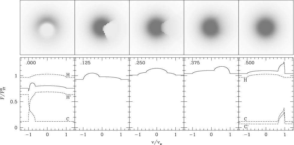
As an example, we show in Fig. 10 (bottom panels) the modelled line plus continuum flux, relative to the continuum flux expected for a one-temperature wind, for a number of orbital phases (measured with respect to the time of superior conjunction of the X-ray source), with the parameters taken from Paper II ($Q_{T}=7$, $i=74^{\circ}$ and $\Theta=34^{\circ}$). Also shown (top panels) is the modelled continuum surface brightness that one would observe if one were able to resolve the source. In the latter, one can see that, in the centre, the hot part of the wind (the one which extends over a larger angle) is brighter (blacker) than the cool part. This is because in these dense regions of the wind, the optical depth is large both in the hot and in the cool part, so that the surface brightness is determined by the Planck function (i.e., proportional to the temperature in the Rayleigh-Jeans tail). Far away from the centre, the surface brightness in the cool part is slightly larger (this is just noticeable in, e.g., the right-hand side of the third panel), since at these distances the wind is optically thin, and the lower temperature is more than compensated for by the larger optical depth. In the leftmost panel, one can see the blocking of the brightest region of the hot part of the wind by the much more opaque cool part.

Figure 11: The model infrared light curve. In the panels, light curves are drawn as a function of orbital phase for $Q_{T}=4$, 7 and 15 for different values of $i$ and $\Theta$ (as indicated). The observed light curve – obtained from the 1992 May K-band spectra (see Paper II) – is overdrawn (filled symbols). Some points are shown shifted by one orbital period as well (open symbols). For all points, the observing times were converted to orbital phase using a time of superior conjunction $t_{0}={\rm{}JD_{bar}}\,2448771.997$, and the fluxes were divided by $F^{\rm{}ff}_{\rm{}1T}=11.373\,$mJy. These values of $t_{0}$ and $F^{\rm{}ff}_{\rm{}1T}$ are the best-fit values for $Q_{T}=7$, $i=74^{\circ}$, and $\Theta=34^{\circ}$ (for the other sets of parameters, they are not very different). The time $t_{0}$ corresponds to X-ray phase $\phi_{\rm{}X}=0.87$. For reference, X-ray minimum occurs at $\phi_{\rm{}X}=0.96$ (Van der Klis & Bonnet-Bidaud [1989])

The line profile is composed of two components that shift in velocity with orbital phase. The broad weak component arises in the hot part of the wind, and the sharp strong one in the cool part. The latter is rather weak at orbital phase 0, when the X-ray source is at superior conjunction and the cool part of the wind is moving most directly towards us (see Fig. 8). The line profile even shows a small absorption feature. This is because in the line the opacity in the cool part of the wind is larger, and hence the absorption of the continuum emission from the hot part of the wind is more effective. Conversely, half an orbit later, when the cool part is moving away from us, the line component arising in it is rather strong. In fact, the red wing is stronger than would be the case if the whole wind were cool, because the intervening continuum opacity in the hot part of the wind is lower than would be the case for a completely cool wind.

In Fig. 11, the predicted infrared light curves are shown for a range of values of the parameters $(Q_{T},i,\Theta)$. For comparison, the light curve derived from the 1992 May spectra is overdrawn (see Paper II), using $F^{\rm{}ff}_{\rm{}1T}=11.373\,$mJy and $t_{0}={\rm{}JD_{bar}}\,2448771.997$ as derived from fitting the lightcurve to the model with $Q_{T}$ held fixed at 7 (Paper II). The best-fit values of these two parameters hardly vary with the choice of $(Q_{T},i,\Theta)$. From the figure, it is clear that the infrared light curve does not uniquely determine $Q_{T}$, $i$ and $\Theta$. The parameter combinations that yield the most satisfactory fit to the observed light curve are those with with $(Q_{T},i,\Theta)=(4,90^{\circ},41^{\circ})$, $(7,74^{\circ},34^{\circ})$ and $(15,66^{\circ},30^{\circ})$.

Figure 12: Observed and modelled Line profiles at maximum blueshift (lower curves) and at maximum redshift (upper curves). In the rightmost panel, three observed He ii $(10-7)$ profiles are shown (taken from Fig. 7). The fluxes of the three profiles have been divided by 10.5, 8.5 and $9\,10^{-15}\,{\rm{}W\,m^{-2}\,\hbox{$\mu$m}^{-1}}$ (top to bottom), and for the conversion to fractional velocity, a wind velocity of 1500 km s^-1 was used. In the other panels, model profiles are shown for five different sets of parameters (as indicated). The drawn curve reflects the model results, and the histogram the results binned to the resolution of the observations (no smoothing over phase was applied)

In Paper II it was shown that the wavelength shifts observed in 1992 May could be reproduced with the model. The wavelength shifts shown in the other observations are very similar to these, and therefore we will not discuss these further, but rather focus on the line shapes predicted by the model, and compare these with the profiles observed in the higher resolution K-band spectra that we now have available.

In Fig. 12, we show the observed profiles for maximum redshift and maximum blueshift, and compare these with the predicted profiles. The latter were calculated for the three parameter sets that produce the best fits to the observed light curve (see above), as well as for two other sets that produce adequate fits and that represent somewhat different positions in parameter space. From the figure, one notices that the modelled lines are weaker at maximum blueshift than at maximum redshift, as discussed above for the example shown in Fig. 10. Small absorption components at maximum blueshift are found in three cases. Their presence reflects the geometry of the model: they are present for values of $\Theta$ slightly larger than $(90^{\circ}-i)$, i.e., for the case in which a significant fraction of the cool matter moving almost directly towards us, is seen projected against the hot part of the wind. For $\Theta$ significantly larger than $(90^{\circ}-i)$, the optically thick central region of the cool part of the wind intervenes.

In comparing the modelled profiles with the observed ones in more detail, one should keep in mind that $K^{\rm{}line}$, which determines the strength of the line, has been kept the same for all models. For the value chosen, the line would peak at 40% above the continuum if the whole wind were cool. The equivalent width would be $0.6\,v_{\rm{}w}$, or $\sim\!70(v_{\rm{}w}/1500\,\hbox{km\,s${}^{-1}$})\,\AA$ at He ii $(10-7)$ (where 1500 km s^-1 is the velocity indicated by both the He i and He ii line profiles; see Sect. 5 below). In WN6/7 stars, equivalent widths ranging from 30 to 130 Å are observed, with the stronger lines occurring in WN6 stars (Hillier et al. [1983]; Hillier [1985]). Hence, differences in the line strength of the order of a factor 2 are to be expected. Keeping this in mind, some conclusions can be drawn from the comparison with the observed profiles. Specifically, the relative strength shown by the model profiles at maximum redshift and the relative weakness at maximum blueshift, is seen in the observed He ii profiles as well, both in the series of K-band spectra obtained in 1992 (Fig. 6) and the one obtained in 1993 (Fig. 7). Furthermore, the asymmetry of the observed profiles is consistent with that expected from the two-temperature structure of the wind.

From a closer comparison (Fig. 12), one sees that the observed profiles – which are clearly resolved – are best reproduced for relatively large values of the opening angle and for values of the inclination not too close to $90^{\circ}$ (note, however, that, given the integration times of 20–30 minutes, the observed profiles represent averages over a range of about 0.1 in orbital phase, and thus are expected to be somewhat broader than the modelled ones). From the different profiles somewhat different conclusions about the temperature ratio $Q_{T}$ are inferred. The lower of the two maximum-redshift profiles in Fig. 12 shows hardly any blue-shifted emission, and from this profile one would thus infer a high value of $Q_{T}$. In contrast, the maximum-blueshift profile (taken in the same run) and the other maximum-redshift profile (taken a year earlier) show profiles from which a lower value $Q_{T}$ would be indicated. Given both the difficulty in determining the observed ratio due to the uncertainty in the continuum level, and the simplicity of the model, it seems that differences like these are to be expected, and that, in general, the characteristic variations shown in the observed profiles (Sect. 3.3) can be adequately reproduced.

5 Wind velocity and mass-loss rate

For a constant-velocity, isothermal wind, the free-free flux depends only on the ratio of the mass-loss rate $\dot{M}$ and the velocity $v_{\rm{}w}$ of the wind ($\dot{M}/v_{\rm{}w}\propto F^{3/4}$; Wright & Barlow [1975]). In Paper II, the relations given by Wright & Barlow ([1975]) and Hillier et al. ([1983]) were used to estimate the mass-loss rate in Cyg X-3. With the parameter $F^{\rm{}ff}_{\rm{}1T}$ determined from the fit to the 1992 May infrared light curve, corrected for 1.5 magnitudes of interstellar extinction as derived by Becklin et al. ([1972]), and the wind velocity determined from the wavelength shifts, a mass-loss rate $\dot{M}_{\rm{}ff}=4\,10^{-5}\,\hbox{M${}_{\odot}$}\,{\rm{}yr^{-1}}$ was derived (for a distance of 10 kpc, and assuming completely ionised helium and a gaunt factor of unity; cf. Hillier et al. [1983]).

Another estimate of the mass-loss rate can be made on the basis of the observed increase of the orbital period, as was done in Paper I, if one assumes that the specific angular momentum carried away by the wind is equal to that of the helium star. With the orbital parameters of Kitamoto et al. ([1995]), we find $\dot{M}_{\rm{}dyn}=M_{\rm{}tot}\dot{P}/2P=0.6\,10^{-5}(M_{\rm{}tot}/10\,\hbox{M${}_{\odot}$})\,\hbox{M${}_{\odot}$}\,{\rm{}yr^{-1}}$, where $M_{\rm{}tot}$ is the total mass of the system. Hence, for reasonable values of the mass of the helium star ($\sim\!10\,\hbox{M${}_{\odot}$}$) and the compact object ($1.4\,\hbox{M${}_{\odot}$}$), $\dot{M}_{\rm{}dyn}$ is smaller than $\dot{M}_{\rm{}ff}$ by about a factor of 6. This discrepancy may well be larger, since, as shown below, the present observations indicate that $\dot{M}_{\rm{}ff}$ may have been underestimated in Paper II.

In Paper II, a wind velocity of 1000 km s^-1 was used to estimate $\dot{M}_{\rm{}ff}$. From the observations presented here, it is possible to derive a more accurate estimate of the wind velocity. Williams & Eenens ([1989]) have argued that a reliable estimate of the terminal velocity of the wind can be obtained from the blue edge of blue-shifted absorption features of the He i $\lambda 2.058$ line, such as we have observed in the K-band spectra taken on 1993 July 15 (Fig. 7). For both spectra in which the feature is unambiguously detected (the second and third), we find a centroid velocity of $-1200\pm 100\,\hbox{km\,s${}^{-1}$}$. The full widths at half maximum are $800\pm 150$ and $1000\pm 200\,\hbox{km\,s${}^{-1}$}$, respectively. Hence, for the blue edge of the absorption feature we find, after correction for the resolution of the spectra ($\sim\!450\,\hbox{km\,s${}^{-1}$}$), $-1500\pm 200$ and $-1600\pm 250\,\hbox{km\,s${}^{-1}$}$ for the second and third spectrum, respectively. (Here, possible effects of turbulence have been neglected. See Williams and Eenens ([1989]).)

Another estimate of the wind velocity can be obtained from the widths of the lines at times that they do not show an orbital modulation. In Paper I, it was found that the He ii lines in the 1991 I and K-band spectra had full widths at half maximum (FWHM) consistent with a single value of 2700 km s^-1, with an estimated uncertainty of 200 km s^-1. For the He ii $(5-4)$ lines in the spectra taken on 1993 June 14, we find a FWHM of $2800\pm 300\,\hbox{km\,s${}^{-1}$}$. In order to find the velocity to which these widths correspond, we have to make an assumption about the intrinsic line profile. Torres et al. ([1986]) find that, for a line with a parabolic shape, the conversion factor $C_{\rm{}vel}\equiv v_{\rm{}w}/$FWHM equals 0.71, while for a line with a rectangular profile, it is 0.5. For the profile of a line in LTE arising in a one-temperature wind, we find that $C_{\rm{}vel}=0.57$. Of course, these estimates only apply for well-resolved lines. For our spectra, with a resolution of $\sim\!500\,\hbox{km\,s${}^{-1}$}$ in the I band, and $\sim\!900\,\hbox{km\,s${}^{-1}$}$ in the K band, we find that $C_{\rm{}vel}$ for the one-temperature profile should be increased to $\sim\!0.6$. Using $C_{\rm{}vel}=0.6\pm 0.1$ as a conservative estimate, we find that the observed FWHMs of the He ii lines correspond to a wind velocity $v_{\rm{}w}=1650\pm 300\,\hbox{km\,s${}^{-1}$}$.

The maximum velocity shown by the modulated profiles can also be used to estimate the wind velocity. In the 1993 K-band spectra, (Fig. 7; also Fig. 12) emission is seen out to a redshift of $1500\pm 150\,\hbox{km\,s${}^{-1}$}$. After correction for the resolution of $\sim\!450\,\hbox{km\,s${}^{-1}$}$, we find a velocity of $1450\pm 150\,\hbox{km\,s${}^{-1}$}$.

The estimates mentioned above indicate a wind velocity of $\sim\!1500\,\hbox{km\,s${}^{-1}$}$, rather than the 1000 km s^-1 used in Paper II. This velocity is consistent with that expected for a WN6/7 Wolf-Rayet star (e.g., Eenens & Williams [1994]). If the wind velocity is the same in the continuum-forming regions (i.e., if the assumption of a constant velocity is valid), then with the new velocity the mass-loss rate mentioned above will increase by a factor 1.5.

Another uncertainty in the estimate of the mass-loss rate stems from the variability by up to a factor 2 of the phase-averaged infrared intensity of the source. From the spectra that we have available now, it seems likely that the intensity of the source is systematically lower when the lines are weak. In terms of our model, the wind is most ‘Wolf-Rayet like’ when the lines are strong, and therefore the mass-loss rate might be underestimated if one uses, as in Paper II, the flux estimate derived from the weak-line 1992 May spectra. Adopting the flux observed in the 1991 June spectrum, the inferred mass-loss rate would increase by another factor 1.5.

For the interstellar extinction $A_{\rm{}K}$ in the K band, a value of 1.5 magnitudes was used. This value was derived by Becklin et al. ([1972]) from the infrared colours of Cyg X-3, under the assumption that the intrinsic colour $H-K\la 0.3$. However, as we will show below (Sect. 7), the shape of the infrared continuum indicates $A_{\rm K}\simeq 2.0$. Hence, the intrinsic flux may have been underestimated in Paper II. For an increase of 0.5 magnitudes in $A_{\rm{}K}$, the estimate of the mass-loss rate increases by a factor 1.4.

In summary, the estimate of the mass-loss rate $\dot{M}_{\rm{}ff}$ given in Paper II should be considered as a lower limit. If all three corrections mentioned above were to apply, $\dot{M}_{\rm{}ff}$ would increase by a factor 3, to $1.2\,10^{-4}\,\hbox{M${}_{\odot}$}\,{\rm{}yr}^{-1}$, an order of magnitude larger than the dynamical estimate $\dot{M}_{\rm{}dyn}$.

Interestingly, for WR 139 (V444 Cyg), a Wolf-Rayet binary for which a dynamical estimate of the mass-loss rate is available, this estimate is lower by about a factor 3 than the estimates based on the free-free radio emission and on the modelling of the infrared spectral lines (St-Louis et al. [1993], and references therein). For this system, St-Louis et al. ([1993]) find additional evidence for the lower mass-loss rate from polarisation measurements. They suggest that the discrepancy might result from inhomogeneities in the wind. Since the free-free and (non-resonance) line emission processes depend on the square of the density, these inhomogeneities would lead to enhanced free-free and line fluxes, and hence, when the inhomogeneities are neglected, the mass-loss rate will be overestimated. In contrast, the estimates based on the polarisation depend linearly on the density, and thus are independent of these inhomogeneities (provided the wind is optically thin to electron scattering).

Additional evidence that the mass-loss rates in Wolf-Rayet stars may be lower than is inferred from line and free-free continuum fluxes, comes from the profiles of strong He ii lines (e.g., He ii $(3-2)\,\lambda 1640$, He ii $(7-4)\,\lambda 5411$). For these lines, the electron-scattering wings predicted by model calculations tend to be stronger than those observed by a factor of $\sim\!2$ (Hillier [1990]). Hillier ([1990]) suggests that this discrepancy, like the one mentioned above, reflects the presence of inhomogeneities in the wind, due to which the line emission processes – which scale with the density squared – are enhanced, while the electron scattering process – which scales linearly with the density – is not. In order to test this expectation, Hillier ([1991]) performed exploratory model calculations on an inhomogeneous wind. He found that, indeed, lines as strong as those obtained for a homogeneous wind, but with electron-scattering wings in accordance with the observations, could be obtained, for a mass-loss rate that was about half that needed for a homogeneous wind.

From the above, we conclude that the mass-loss rate $\dot{M}_{\rm{}ff}$ of $\sim\!10^{-4}\,\hbox{M${}_{\odot}$}\,{\rm{}yr}^{-1}$ that is inferred from the infrared flux, should be regarded as a highly uncertain estimate of the genuine mass-loss rate $\dot{M}_{\rm{}true}$. From the cases discussed above, it follows that $\dot{M}_{\rm{}true}$ may be smaller than $\dot{M}_{\rm{}ff}$ by a factor of 2–3. For Cyg X-3, it seems not unlikely that the difference is even larger, since possible inhomogeneities may well be enhanced as a result of its variable nature. The conclusions drawn in the previous section are not necessarily affected, however, provided the inhomogeneity of the wind is similar in both the hot and the cold part of the wind.

6 Ramifications

In this section, we discuss qualitatively the complications that arise for cases in which one or more of the assumptions underlying our model are invalid. We start with the main assumption, viz., that the size of the continuum and line emitting regions is much larger than both the orbital separation and the size of the regions of the wind where significant velocity and temperature gradients are present (Sect. 4.1). Thereafter, we briefly discuss the effects of the rotation of the system, of the contribution of bound-free processes to the absorption opacity, and of electron scattering.

6.1 The size of the continuum and line emitting regions

Wright & Barlow ([1975]) define the characteristic radius of the free-free emitting region by the condition that the integrated flux emitted exterior to that radius (i.e., without optical-depth effects) equals the flux from the whole wind (including optical-depth effects). At this radius, the radial optical depth to infinity is 0.244. It is given by

$$R^{\rm ff}_{\rm char} =8.8 \left(\frac{\dot{M}_{\rm ff}}{10^{-4}\,\hbox{M${}_{\odot}$}\,{\rm yr}^{-1}}\right)^{2/3}\left(\frac{v_{\rm w}}{1500\,\hbox{km\,s${}^{-1}$}}\right)^{-2/3}\times$$ (1)

$$\left(\frac{\lambda}{2.2\,\hbox{$\mu$m}}\right)^{2/3}\left(\frac{T}{5\,10^{4}\,{\rm K}}\right)^{-1/2}\,\hbox{R${}_{\odot}$}.$$

Here, the mass-loss rate $\dot{M}_{\rm{}ff}$ and the wind velocity $v_{\rm{}w}$ were scaled to the values found in Sect. 5, and the temperature $T$ to an estimate of the temperature in the cool part of the wind. We have used a mass-loss estimate of $10^{-4}\,\hbox{M${}_{\odot}$}\,{\rm{}yr^{-1}}$ for $\dot{M}_{\rm{}ff}$, which we argued above might be influenced by the presence of inhomogeneities, since, for the estimate of the free-free radius, we want to include these effects. Note that the effective radius of the wind, defined by $F^{\rm ff}=4\pi B(T)R_{\rm{}eff}^{2}$, is at a radial optical depth to infinity of 0.05 (Hillier et al. [1983]), and that it is a factor 1.7 larger than the characteristic radius defined above.

From the temperature dependence of the characteristic radius, it is clear that the assumption that it is large compared to the other relevant sizes, will break down first in the high-temperature part of the wind. Taking the size of the Roche lobe of the helium star – 1.7 R_⊙ for a 10 M_⊙ helium star and a 1.4 M_⊙ compact object (Paper I) – as an optimistic estimate of the value of the characteristic radius below which the assumptions will break down, we find that the critical value $Q_{\rm{}crit}$ of the temperature ratio is 27 in the K band (for the values of $\dot{M}_{\rm{}ff}$, $v_{\rm{}w}$ and $T$ used in Eq. 1). As a more pessimistic estimate, the orbital separation can be used, which, for the masses quoted above, is 3.2 R_⊙. The value of $Q_{\rm{}crit}$ corresponding to this radius is 8. For the I band ($0.9\,\hbox{$\mu$m}$), the values for the two cases are $Q_{\rm{}crit}=8$ and 2.3, respectively.

The estimates of the critical values of $Q_{T}$ are within the range of values that we have used for our model. Hence, it is likely that deviations from the model results discussed above occur. For the wind of the helium star, one expects that both the assumption that the wind is isothermal, and the assumption that is has a constant velocity, will not be valid close to the star. Furthermore, the assumption that the shadow can be represented as a cone with the helium star at its vertex, will break down. We will discuss these three points in turn.

Temperature.

Close to the surface of the helium star, where the X rays cannot penetrate, the temperature of the wind will be determined by the helium-star properties alone, and thus be lower than assumed in our model. To obtain a crude estimate of the consequences, we consider the case where outside of a certain radius $R_{\rm{}b}$ the wind is strongly heated, and within that radius not at all. At very long wavelengths, the heated part of the wind will be optically thick, and our model assumptions apply. However, going to shorter wavelengths, the heated part will become optically thin, and the cooler layers below will become visible. In these layers, the optical depth is much higher, and thus these layers will effectively appear as a blackbody of radius $R_{\rm{}b}$, with the temperature determined by the helium star properties. Hence, the spectrum will flatten, then steepen at shorter wavelengths as the wind ceases to contribute, and finally flatten at still shorter wavelengths when the cooler layers become transparent.

Velocity.

For high values of $Q_{T}$, one will observe the deeper, accelerating layers of the wind (see Fig. 8). Since the velocity in these layers is lower, the density and thus the free-free opacity will be higher. In consequence, the effects will be opposite to those discussed for the temperature above: the flux will be higher, and, since this effect will be stronger at shorter wavelengths, the spectrum will be steeper than is expected for a constant-velocity wind.

Geometry

The assumption that the wind is confined within a cone with the helium star at its vertex, will also cease to be realistic for high values of $Q_{T}$. From trial calculations on a two-temperature wind with a genuine shadow (see Fig. 8), we found that, indeed, for high values of $Q_{T}$, the light curves differ significantly (mostly showing a wider minimum), due to the very dense parts of the wind, well within a stellar radius of the star, now becoming shadowed and thus cool. However, since close to the star the assumption of a constant temperature and a constant velocity will also be invalid (see above), we do not consider these results as better than the ones obtained with our model in its simplest geometric form.

6.2 Rotation

Due to the orbital motion in the system, the matter in the wind of the helium star will start to trail the star at larger radii. Hence, in assuming that the cool part is within a cone, we implicitly assume that both the cooling in the shadow, and the X-ray heating outside are very fast. If this is not the case, the cool part of the wind will be lagging at larger radii. An observational indication that this may in fact happen, is that the X-ray light curve shows an asymmetric minimum, with a rather steep ingress and a more moderately-sloped egress. In the infrared, a similar effect may be present. For instance, the infrared light curve observed by Mason et al. ([1976]), shows an ingress that is steeper than the egress. The K-band light curve we observed, is more symmetric (Fig. 11), but from the points in the phase interval $-0.26$ to $-0.2$, it does appear that ingress is somewhat faster than egress.

6.3 Bound-free opacity

Another effect that we have neglected in our model, is the contribution of the bound-free process to the opacity. Since this contribution decreases with increasing temperature, one may expect that, going from a one-temperature to a two-temperature state, the infrared flux will decrease. Hillier et al. ([1983]) found that, for a temperature of 50000 K, the contribution of the bound-free opacity to the total opacity is $\sim\!15\%$ of that of the free-free opacity in the K band and $\sim\!45\%$ in the I band. At 30000 K – a reasonable lower limit to the temperature in the cool part – the relative contributions are $\sim\!25\%$ and $\sim\!80\%$, respectively. However, Hillier et al. also note that the effect is almost cancelled by the error made in assuming the Rayleigh-Jeans approximation. (For instance, at 0.9 $\mu$m and 50000 K, both the black-body flux and the free-free opacity are about 15% lower than expected in the Rayleigh-Jeans approximation, leading to a 25% decrease in expected flux.) Hence, it seems unlikely that with the inclusion of bound-free opacity in the model, one would be able to reproduce the observed changes in the continuum of up to a factor 2 in both the I and K bands.

The contribution of the bound-free opacity might also reflect itself in an increased depth of the modulation, since, due to its contribution, the cool part of the wind should be more opaque, while the hot part should not. Given the wavelength dependence of this contribution, any effect should be stronger at shorter wavelengths, and one would, therefore, expect that the depth of the modulation would increase going to shorter wavelengths. The observational evidence on this is confused: Fender & Bell-Burnell ([1994]) find that the depth of the modulation is larger at H than at K, but Molnar ([1988]) finds that there are no colour changes with orbital phase.

6.4 Electron scattering

Electron scattering will be important if the radius at which $\tau_{\rm{}es}\simeq 1$ exceeds the characteristic radius $R^{\rm{}ff}_{\rm{}char}$ of the free-free emitting region. For constant-velocity, spherically-symmetric mass loss, this radius is given by

$$R_{\rm es}=9.6\left(\frac{\dot{M}}{10^{-4}\,\hbox{M${}_{\odot}$}\,{\rm yr}^{-1}}\right)\left(\frac{v_{\rm w}}{1500\,\hbox{km\,s${}^{-1}$}}\right)^{-1}\,\hbox{R${}_{\odot}$}.$$ (2)

Hence, for the free-free mass-loss rate of $\sim\!10^{-4}\,\hbox{M${}_{\odot}$}\,{\rm{}yr}^{-1}$ (Sect. 5), electron scattering will be important in both the hot and the cold parts of the wind. However, as discussed in Sect. 5, the genuine mass-loss rate $\dot{M}_{\rm{}true}$, with which the electron scattering optical depth scales, is most likely lower by at least a factor 2–3. For such a lower estimate, $R_{\rm{}es}\simeq 3$–5 R_⊙, and electron scattering will be important in the hot part of the wind for $Q_{T}\ga 3$–8. Due to the electron scattering, the hot part of the wind will appear more extended. Hence, the depth of the modulation will decrease somewhat, and the minimum will become somewhat wider.

At the radial distance of the X-ray source ($a\simeq\!3\,\hbox{R${}_{\odot}$}$; see above), the electron scattering optical depth to infinity will be $\ga\!1$ even when the mass-loss rate estimate is decreased by a factor 2–3. Thus, the X-ray source will effectively be larger, and the shadow of the helium star will become less well-defined, especially at larger radii. One may expect that, in these less shadowed regions, the degree of ionisation will be increased. This may explain the absence of He i emission in the spectra with weak, modulated lines.

7 The continuum energy distribution

If the hypothesis that the infrared continuum and lines in Cyg X-3 originate from a Wolf-Rayet wind, is correct, it is to be expected that the continuum energy distribution is similar to that observed in Wolf-Rayet stars, i.e., that it can be described by a power-law of the form $F_{\nu}\propto\nu^{\beta}$ (Morris et al. [1993]; see Sect. 4.1). To test this expectation, and also to look for possible deviations that might result from the break down of the assumptions underlying our model (as discussed above), we collected photometric data from the literature, and combined these with the our spectroscopic results. For this purpose, the K-band spectra can be used directly, since these are flux calibrated. This is not the case for our I-band spectra. However, since these were reduced relative to the nearby star A (see Sect. 2.1), for which photometry is available, we can obtain an estimate of the fluxes using star A as a local standard.

Figure 13: The continuum flux distribution. Shown are the fluxes derived from the JHKL photometry of Molnar ([1988]), and from our spectra. The lower set of points and curves ($A_{\rm{}J}=0$) reflects the observed data. The JHKL points are connected by a dashed line to indicate that they were obtained simultaneously. Two K-band spectra are shown, the spectrum with strong lines obtained on 1991 June 29, and the weak-line average spectrum obtained on 1992 May 29. In the I-band, the strong-line average spectrum obtained on 1993 June 14 is shown, the weak-line average spectrum obtained on 1992 July 25, and, to extend the wavelength range to smaller wavelengths, the strong-line spectrum obtained on 1991 June 21 (notice that, for the latter, the flux level may be underestimated; see Sect. 2.1). The other sets of points and curves reflect the data corrected for the interstellar extinction for three different values of $A_{\rm{}J}$ (as indicated). The extinction law we used was that of Mathis ([1990]). For the IJHKL bands, this extinction law gives $A_{\lambda}\propto\lambda^{-1.7}$. For comparison, the flux-calibrated I, J and K-band spectra of WR 134 (WN6), corrected for interstellar extinction using $A_{\rm J}=0.69$ (Morris et al. [1993]), are shown at the top (shifted upward by 0.5 dex for clarity)

For star A, Westphal et al. ([1972]) list $V=15.05$, $B-V=0.98$ and $U-B=0.43$. From our spectra, we found that the spectral type is in the range F5 to G0 (Sect. 2.1). From the observed colours, we conclude that the star cannot be a supergiant. For main-sequence stars of the above-mentioned range in spectral type, the effective temperatures range from 6400 to 5900 K, and the intrinsic colours $\{(U-B)_{0},(B-V)_{0},(V-I)_{0}\}$ range from $\{0.00,0.43,0.64\}$ to $\{0.11,0.59,0.81\}$ (Johnson [1966]). With the interstellar extinction law given by Mathis ([1990]), the $E_{B-V}$ and $E_{U-B}$ colour excesses correspond to values of the interstellar extinction at J ranging from $A_{\rm{}J}=0.48$ to 0.34, and from $A_{\rm{}J}=0.52$ to 0.39, respectively. [Note that the interstellar extinction law of Mathis ([1990]) is normalised at J. This band is chosen because longward of $\sim\!1\,\hbox{$\mu$m}$ the extinction law is virtually identical in all lines of sight.] Hence, the expected Johnson I magnitude ranges from 13.52 to 13.59.

For the flux calibration, we assume that, in the wavelength range covered by our spectra, star A can be represented by a black body of 6000 K, reddened by interstellar extinction corresponding to $A_{\rm{}J}=0.4$, and scaled to produce an I-band magnitude of 13.55 (these values are appropriate for spectral type F8). To estimate the accuracy of this procedure, we also calibrated our WHT I-band spectra of the Wolf-Rayet stars, and compared these with the J-band spectra obtained at UKIRT. We found that the flux calibration was accurate to $\sim\!20\%$, with no obvious systematic offsets, and that the differences in the power-law slope $\beta$ of the spectra were less than $\sim\!0.1$.

Figure 13 shows the observed flux distribution derived from our spectroscopy, as well as from photometry in JHKL by Molnar ([1988]). The figure also shows the flux distributions corrected for three different amounts of interstellar extinction, corresponding to $A_{\rm{}J}=4$, 5.5, and 7. As above, we used the reddening law of Mathis ([1990]). For wavelengths longward of 0.8 $\mu$m, this extinction law is equivalent to $A_{\lambda}\propto\lambda^{-\alpha}$, with $\alpha=1.7$. For comparison, we also show our I, J and K-band spectra of WR 134 (WN6), dereddened using $A_{\rm{}J}=0.69$ ($E_{B-V}=0.47$; Morris et al. [1993]).

From the figure, it is clear that the shape of the intrinsic flux distribution of Cyg X-3 is very sensitive to the assumed amount of interstellar reddening. In order to obtain a flux distribution that neither starts to fall at shorter wavelengths, nor becomes steeper than the Rayleigh-Jeans tail of the Planck function, the value of $A_{\rm{}J}$ should be larger than 4 and smaller than 7. From more detailed plots, we find that, in order to have $-0.3\la\beta_{\rm{}\/I}\la 2$ for the I-band spectra, one needs $5\la A_{\rm{}J}\la 6$. [Here, $\beta=-0.3$ corresponds to optically thin free-free emission.] For this range, the power-law index as derived from the longest wavelengths (i.e., K, L), varies from $\beta_{K-L}=1.2$ to 1.6. For $A_{\rm{}J}=5.5$, the whole flux distribution longward of $0.8\,\mu$m is consistent with $\beta_{\lambda>0.8}=1.4$.

An uncertainty in the above derivation is introduced by the uncertainty of about 0.1 in the index $\alpha$ used in the extinction law (Mathis [1990]). We find that, to have $-0.3\la\beta_{\rm\/I}\la 2$ for $\alpha=1.8$, the range in $A_{\rm{}J}$ has to decreased by $\sim\!0.1$, $\beta_{K-L}$ by $\sim\!0.2$, and $\beta_{\lambda>0.8}$ by $\sim\!0.2$. For $\alpha=1.6$, the range in $A_{\rm{}J}$ has to be increased by $\sim\!0.3$, and $\beta_{K-L}$ by $\sim\!0.1$. For this value of $\alpha$, it is not possible to fit the whole spectrum well with a single power-law, but to a reasonable approximation $\beta_{\lambda>0.8}\simeq 1.9$.

In summary, under the assumption that $-0.3\la\beta_{\rm{}I}\la 2$, we find that $A_{\rm{}J}=5.5\pm 0.6$. This value corresponds to a K-band extinction of $A_{\rm K}=2.1\pm 0.4$. For $A_{\rm{}J}\simeq 5.5$, the flux distribution for $\lambda>0.8\,\hbox{$\mu$m}$ has a power-law shape, with $\beta_{\lambda>0.8}=1.4\pm 0.3$. This value is higher than predicted by our model ($\beta=2/3$; see Sect. 4.1), but not inconsistent with the values found for normal Wolf-Rayet stars. In the sample of 78 Wolf-Rayet stars studied by Morris et al. ([1993]), 6 have $\beta\geq 1.4$, and 20 have $\beta\geq 1.1$. Since we do not see a strong variation in slope between the strong and the weak-line spectra (Figs. 13, 2 and 5), the large slope we observe is unlikely to be related to the breakdown of the model for high values of the temperature ratio $Q_{T}$. Instead, it more likely reflects the fact that, in general, the model is too simple to provide a detailed description of a Wolf-Rayet wind.

8 Discussion and conclusions

The first infrared spectroscopic observations of Cyg X-3 (Paper I) showed the presence of Wolf-Rayet emission features in the infrared spectrum of Cyg X-3, which indicates that a strong, dense, helium-rich wind is present in the system, in which both the infrared lines and continuum originate. In follow-up observations, the emission lines were much weaker, and they shifted in wavelength as a function of orbital phase (Paper II). It was argued that this could be understood in the context of the helium-star model, if the Wolf-Rayet wind is sometimes strongly ionised and heated by the X rays originating from the compact object. Furthermore, it was argued that if this were the case, the observed modulation of the infrared continuum would follow as a natural consequence. In support of this argument, it was shown that observed variations could be reproduced with a simple model of the system, in which the wind has a two-temperature structure.

In this paper, we have presented a number of additional observations. These observations confirm the prediction made in Paper II that the emission lines show wavelength shifts as a function of orbital phase if they are weak, but not if they are strong. We have described the model used in Paper II in detail, and presented model continuum light curves and model line profiles for various combinations of the parameters. From these results, we have found that from the assumption of a two-temperature wind it follows naturally not only that the lines shift in wavelength, but also that the profiles at maximum redshift are stronger and narrower than at maximum blueshift.

A problem we have encountered, is that the estimate of mass-loss rate inferred from the infrared flux is an order of magnitude larger than the estimate inferred from the rate of increase of the orbital period. We have also found that the observed flux distribution is not consistent with the model. However, since similar deviations are found for normal Wolf-Rayet stars, we believe that these discrepancies reflect the simplifications made for our model, and that they do not invalidate our main conclusions, viz., that the continuum and the lines arise in the wind of the helium star, and that the modulation of both lines and continuum is due to the wind being highly ionised by the X-ray source, except in the helium star’s shadow.

An open question that remains is what the underlying cause is of the changes in state, in the infrared as well as in X-ray and radio. Watanabe et al. ([1994]) have found that the radio and X-ray states are correlated: large radio outbursts occur when the X-ray source is in its high state (high flux, soft spectrum), but not when it is in its low state (low flux, hard spectrum). Kitamoto et al. ([1994]) determined that the radio/X-ray source was in its high state in June 1991, when the infrared spectra showed strong lines, and in its low state in May 1992, when the lines were weak. They suggested that the state at all wavelengths was a function of the mass-loss rate of the Wolf-Rayet star only. When high, the infrared continuum would be stronger and the accretion rate would be high, leading to a strong X-ray source and radio outbursts (the latter are presumably due to the ejection of relativistic jets; e.g., Geldzahler et al. [1983]). The wind would be dense enough to be optically thick to low-energy X rays, leading to a low state of ionisation. When the mass-loss rate was lower, the infrared continuum flux and the accretion rate would be low, leading to X-ray low state and the absence of radio outbursts. They suggested that the wind would become optically thin to low-energy X rays, so that it could be ionised despite the lower X-ray luminosity.

At present, the hypothesis of a variable wind mass-loss rate as the underlying cause of the changes in state is consistent with the observations. Other Wolf-Rayet stars of the WN subclass, however, do not show evidence for large changes in mass-loss rate, showing, e.g., constant flux to within a few percent on all observed time scales (Moffat & Robert [1991]). It might be that the changes in accretion rate and optical depth that are required are due to processes near the X-ray source and its accretion disk, perhaps similar to those underlying the changes in state observed in black-hole candidates like Cyg X-1 (e.g., Oda [1977]).

One possibly major problem that has been addressed only briefly so far (in Paper I) is that the radii of Wolf-Rayet stars derived from model fits to Wolf-Rayet spectra (e.g., Schmutz et al. [1989]), are much larger than the radius of the Roche lobe in Cyg X-3 (Paper I; Conti [1992]). Schmutz ([1993]) has tried to model the 1991 I and K-band spectra of Cyg X-3 using the Wolf-Rayet wind model described by Hamann & Schmutz ([1987]) and Wessolowski et al. ([1988]). He found that the stellar parameters were typical for a Wolf-Rayet star of spectral type WN7, but that given the absolute K magnitude, the photospheric radius was larger than the orbital separation by a factor 3. In order to resolve this discrepancy, he suggested that the distance to Cyg X-3 was much smaller than 10 kpc, so that the luminosity, and thus the mass and radius, were much smaller. He suggested that the 21 cm absorption features, on which the 10 kpc distance is based, might be due to circumstellar shells.

Although the suggestion of a lower distance is tempting in that it would also resolve the discrepancy between the different estimates of the mass-loss rate, we believe that it is unlikely that there are circumstellar shells at such velocities and with such strengths that they produce a 21 cm absorption profile which corresponds closely with the combined emission profile of the Local, Perseus and Outer arms (e.g., Dickey [1983]). Instead, we believe it more likely that the estimate of the radius derived from the model-atmosphere fits is wrong. We stress that these estimates are based on an assumed velocity law, which is used to extrapolate inward from the regions where the continuum and lines are formed, to the so-called ‘zero-velocity’ radius. Usually, for this velocity law, a $\beta$-law is used ($v=v_{\infty}(1-R_{*}/r)^{\beta}$). This velocity law has been found to be a reasonable approximation for O stars, but there is no reason to assume it is valid for Wolf-Rayet stars as well, especially close to the star (for more thorough discussions, we refer to Kudritzki & Hummer [1990]; Hillier [1995]; Schmutz [1995]).

An observational indication that the radii of Wolf-Rayet stars are actually quite small comes from studies of Wolf-Rayet stars in eclipsing binaries. For instance, Cherepashchuk et al. ([1984]) found that the eclipse light curve of V444 Cyg indicated a core radius (electron-scattering optical depth unity) of only 2.8 R_⊙. Hamann & Schwartz ([1992]) argue that this estimate is not unique, and that the radius of the Wolf-Rayet star could be much larger. From polarisation measurements, however, St-Louis et al. ([1993]) find that radii larger than $\sim\!4\,\hbox{R${}_{\odot}$}$ are excluded. A similar conclusion is reached by Cherepashcuk et al. ([1995]) based on a spectroscopic estimate of the luminosity ratio. Using this and other observational evidence, Moffat & Marchenko ([1996]) conclude that the radii of Wolf-Rayet stars are not unlike the radii expected from stellar model calculations (e.g., Langer [1989]). For such radii, the helium star would fit well inside the Roche lobe in Cyg X-3 (Paper I).

We conclude from our data that the idea that the companion of Cyg X-3 is a massive Wolf-Rayet star is entirely plausible. It seems to us that Cyg X-3 is a very interesting system, in which a Wolf-Rayet wind can be probed through the combined effects of occultation and variable ionisation by X rays.