Abstract

The observation of air showers from elementary particles with energies exceeding $10^{20}{\,{\rm eV}}$ poses a puzzle to the physics and astrophysics of cosmic rays which is still unresolved. Explaining the origin and nature of these particles is a challenge. In order to constrain production mechanisms and sites, one has to account for the processing of particle spectra by interactions with radiation backgrounds and magnetic fields on the way to the observer. In this paper, I report on an extensive study on the propagation of extragalactic nucleons, $\gamma$-rays, and electrons in the energy range between $10^{8}{\,{\rm eV}}$ and $10^{23}{\,{\rm eV}}$. I have devised an efficient numerical method to solve the transport equations for cosmic ray spectral evolution. The universal radiation background spectrum in the energy range between $\simeq 10^{-9}{\,{\rm eV}}$ and $\simeq 1{\,{\rm eV}}$ is considered in the numerical code, including the diffuse radio background, the cosmic microwave background, and the infrared/optical background, as well as a possible extragalactic magnetic field. I apply the code to compute the particle spectra predicted by various models of ultrahigh energy cosmic ray origin. A comparison with the observed fluxes, especially the diffuse $\gamma$-ray background in several energy ranges, allows one to constrain certain classes of models. I conclude that scenarios which attribute the highest energy cosmic rays to Grand Unification Scale physics or to cosmological Gamma Ray Bursts are viable at the present time.

PACS numbers: 98.70.Sa, 98.70.Rz, 98.80.Cq

1 Introduction

Shortly after the cosmic microwave background (CMB) was discovered [1] it became clear that this universal radiation field has profound implications for the astrophysics of ultrahigh energy cosmic rays (UHE CR) of energies above $10^{18}{\,{\rm eV}}$. For nucleons the most profound effect is photoproduction of pions on the CMB. Known as the Greisen-Zatsepin-Kuz’min (GZK) “cutoff” [2, 3], this effect leads to a steep drop in their energy attenuation length by about a factor 100 at around $6\times 10^{19}{\,{\rm eV}}$ which corresponds to the threshold for this process. The nucleon attenuation length above this threshold is about $10{\,{\rm Mpc}}$. Heavy nuclei with energies above about $10^{19}{\,{\rm eV}}$ are photodisintegrated in the field of the CMB within a few ${\,{\rm Mpc}}$ [4]. One of the major unresolved questions in cosmic ray physics is the existence or non-existence of a cutoff in the UHE CR spectrum at a few $10^{19}\,$eV which, in the case of extragalactic sources, could be attributed to these effects.

Therefore, there has been renewed interest in UHE CR research since events with energies exceeding $10^{20}{\,{\rm eV}}$ have been detected. The Haverah Park experiment [7] reported several events with energies near or slightly above $10^{20}{\,{\rm eV}}$. The Fly’s Eye experiment [8, 9] detected the world’s highest energy CR event to date, with an energy $\simeq 3\times 10^{20}{\,{\rm eV}}$. Near the arrival direction of this event the Yakutsk experiment [10] recorded another event of energy $\simeq 1.1\times 10^{20}{\,{\rm eV}}$. More recently, the AGASA experiment [11, 12] has also reported an event with energy $1.7-2.6\times 10^{20}{\,{\rm eV}}$. It is currently unclear whether these events indicate a spectrum continuing beyond $10^{20}{\,{\rm eV}}$ without any cutoff or the existence of a cutoff followed by a recovery in the form of a “gap” in the spectrum [13].

There has been much speculation about the nature and origin of these highest energy cosmic rays (HECRs) [14, 15, 16, 17, 18]. Concerning the production mechanism one can distinguish between two broad classes of models: Within acceleration models, charged primaries, namely protons and heavy nuclei are accelerated to very high energies [19, 20] in a “bottom-up” manner. Preferred sites are large-scale astrophysical shocks which occur for instance in radio galaxies [21]. Even there it seems barely possible to accelerate CRs to the required energies [14, 22, 23]. Recently it has also been suggested that acceleration of UHE CRs could be associated with cosmological gamma-ray bursts (GRBs) [24, 25, 26]. In the second class of so called “top-down” models, charged and neutral primaries are produced at UHEs in the first place, typically by quantum mechanical decay of supermassive elementary X particles related to grand unified theories (GUTs). Sources of such particles at present could be topological defects (TDs) left over from early universe phase transitions caused by the spontaneous breaking of symmetries underlying these GUTs [27, 28, 29, 30, 31, 32, 33, 34]. The injection spectra in top-down models tend to be considerably harder (flatter) than in acceleration models.

The particle identity of the UHE CRs is not known either. The Fly’s Eye analysis [8] suggested a transition from a spectrum dominated by heavy nuclei to a predominantly light composition, i.e. nucleons or even $\gamma$-rays, above a few times $10^{19}{\,{\rm eV}}$. However, this has not been confirmed by the AGASA experiment [36]. Although there have been claims that the shower profile of the highest energy Fly’s Eye event may be inconsistent with a primary photon [37] or even with a proton primary [38], the situation is not settled because of many uncertainties which can affect the shower development in the atmosphere.

Other options discussed for the nature of the HECRs include heavy nuclei and even neutrinos [37]. Heavy nuclei have their own merits because they can be deflected considerably by the galactic magnetic field which relaxes the source direction requirements [8, 11]. In addition, for shock acceleration, heavy nuclei can be accelerated to higher terminal energies because of their higher charge. However, one should note that the range for heavy nuclei is limited to a few Mpc as mentioned above. Neutrinos, on the other hand, do not lose much energy over cosmological distances [39, 40], but by the same token the probability for interacting in the atmosphere is small. Attributing the HECRs to neutrinos would therefore require a neutrino flux at UHEs which is much higher than the observed CR flux at the same energies. This poses severe constraints on the possible sources for these neutrinos [41]. In addition, neutrinos would be expected to give rise to predominantly deeply penetrating showers in the atmosphere.

The production spectrum of UHE CRs is modified during their propagation. There are many studies on nucleon propagation in the literature using analytical [42, 43, 44, 45] as well as numerical approaches [17, 46, 47, 48], and the propagation of heavy nuclei has also been considered [17]. This was mainly motivated by the conventional acceleration models which usually predict UHE CR fluxes to be dominated by these particles. However, secondary $\gamma$-rays and neutrinos can also be produced, for example as decay products of pions created by interactions with various radiation backgrounds at the source or during propagation [47]. Under certain circumstances their flux can become comparable with the primary flux [49]. Furthermore, within TD models $\gamma$-rays are expected to dominate to begin with [50]. A study on $\gamma$-ray propagation in this context has been performed recently [51] using a quantitative treatment on the cascade initiated by UHE photons. In my opinion, however, it suffers from several unrealistic assumptions with respect to the injection scenarios considered. I improve on their treatment of the propagation of $\gamma$-rays. Apart from that I find three reasons to explore UHE $\gamma$-ray propagation in more detail in this paper:

First, due to the absence of threshold effects similar to photopion production which causes the GZK “cutoff” for nucleons, the $\gamma$-ray spectrum is not expected to have a break around $10^{20}{\,{\rm eV}}$. Furthermore, $\gamma$-rays can generate electromagnetic (EM) cascades while propagating rather than being absorbed right away. UHE electrons produced by pair production upscatter background photons and transfer most of the energy back to photons. This effect considerably increases the effective energy attenuation length of the “cascade” photons [52, 53]. At a few times $10^{20}{\,{\rm eV}}$ this attenuation length may be even greater than that for protons which drops precipitously at the threshold for photopion production. Extragalactic $\gamma$-rays could therefore have some potential to produce a recovery beyond the GZK “cutoff”.

Second, in contrast to the case of nucleons, the propagation of $\gamma$-rays is presently fraught by certain ambiguities which are mainly due to uncertainties in the intensity of the universal radio background and the strength and spectrum of the extragalactic magnetic field (EGMF). We hope that an application of the general framework presented here under different assumptions for such parameters could in turn provide some insights into their actual values once the UHE $\gamma$-ray flux is known to some accuracy. This would be in some analogy to the method of using TeV $\gamma$-ray observations to constrain or detect the universal infrared/optical background [54]. In previous work [52] it is shown that, depending on its strength, the large-scale EGMF could produce a feature in the $\gamma$-ray spectrum which might be observable in the future.

Finally, the study of high energy cosmic and $\gamma$-ray propagation can place stringent constraints on the nature and origin of UHE CRs. Such constraints can be obtained by computing the propagation modified spectra especially of lower energy $\gamma$-rays expected within a certain scenario and comparing the predictions with the observed fluxes [49, 55, 56]. At UHEs there are some experimental prospects to distinguish $\gamma$-rays from other primaries in the future, possibly even on an event by event basis [57]. This would allow comparing not only the total fluxes of UHE nucleons, heavy nuclei, and $\gamma$-rays, but also their composition with model predictions.

This motivated the present comprehensive study of propagation of nucleons and $\gamma$-rays and its application to models which attribute UHE CRs to top-down mechanisms within GUT-scale physics or associate them with cosmological GRBs. I explore the energy range of $10^{8}<E<10^{23}{\,{\rm eV}}$. The low end is chosen such that we can draw constraints by comparing the propagated spectra with existing measurements of the diffuse $\gamma$-ray background around $100{\,{\rm MeV}}$ [58, 59, 60]. The high end is chosen beyond the highest CR energies ever observed enabling us to study top-down models. I include not only the CMB but also the diffuse radio background which plays a big role at the highest energies and the infrared/optical (IR/O) background which influences the flux at somewhat lower energies. I also include the EGMF as a free parameter. The propagation of nucleons is also studied with special emphasis on the production of secondary $\gamma$-rays, electrons, and neutrinos.

The rest of the paper is organized as follows: In Section 2, I present the general ingredients of calculating the propagation of extragalactic $\gamma$-rays and nucleons. I discuss the role and nature of the low energy photon background and the EGMF, and explain in detail the implicit method used in solving the transport equations numerically. Section 3 is devoted to the treatment of the relevant interactions of $\gamma$-rays and nucleons. I compare our analysis with other work in Section 4. Section 5 discusses the generic forms of the injection spectra and the source distribution for typical top-down models and the GRB scenario. Results and constraints from the spectra predicted at Earth are presented in detail. In Section 6, I summarize the findings and discuss future prospects.

2 Formalism

2.1 Radiation backgrounds

UHE CRs undergo reactions with the universal diffuse radiation backgrounds permeating the universe [62]. The most relevant among them are the CMB, and the radio and IR/O backgrounds.

Photon primaries of energy $E$ can be absorbed by pair production with a background photon of energy $\epsilon$ if ($c=\hbar=1$ throughout)

$$E\geq E_{\rm th}\equiv\frac{m_{e}^{2}}{\epsilon}=2.611\times 10^{11}\left(\frac{\epsilon}{1{\,{\rm eV}}}\right)^{-1}{\,{\rm eV}}\,.$$ (1)

Therefore, for a typical CMB photon ($\epsilon\sim 10^{-3}{\,{\rm eV}}$) the threshold energy $E_{\rm th}$ is $\sim 3\times 10^{14}{\,{\rm eV}}$, whereas for a typical radio photon ($\epsilon\mathrel{\mathchoice{\lower 3.6pt\vbox{\halign{$\mathsurround=0pt\displaystyle\hfil#\hfil$\cr<\crcr\sim\crcr}}}{\lower 3.6pt\vbox{\halign{$\mathsurround=0pt\textstyle\hfil#\hfil$\cr<\crcr\sim\crcr}}}{\lower 3.6pt\vbox{\halign{$\mathsurround=0pt\scriptstyle\hfil#\hfil$\cr<\crcr\sim\crcr}}}{\lower 3.6pt\vbox{\halign{$\mathsurround=0pt\scriptscriptstyle\hfil#\hfil$\cr<\crcr\sim\crcr}}}}10^{-8}{\,{\rm eV}}$) the threshold is $\mathrel{\mathchoice{\lower 3.6pt\vbox{\halign{$\mathsurround=0pt\displaystyle\hfil#\hfil$\cr>\crcr\sim\crcr}}}{\lower 3.6pt\vbox{\halign{$\mathsurround=0pt\textstyle\hfil#\hfil$\cr>\crcr\sim\crcr}}}{\lower 3.6pt\vbox{\halign{$\mathsurround=0pt\scriptstyle\hfil#\hfil$\cr>\crcr\sim\crcr}}}{\lower 3.6pt\vbox{\halign{$\mathsurround=0pt\scriptscriptstyle\hfil#\hfil$\cr>\crcr\sim\crcr}}}}3\times 10^{19}{\,{\rm eV}}$, thus affecting UHE $\gamma$-rays. Furthermore, since the pair production cross section peaks near the threshold, pair production on the radio background dominates over pair production on the CMB in that energy range although the number density of radio background photons is much smaller than that of CMB photons. On the other hand, the IR/O background affects the lower energy photons for the same reason. The threshold for pair production on the IR/O background lies at about $10^{12}-10^{13}{\,{\rm eV}}$. Similarly, the contribution of the IR/O background to the total photopion production rate by protons is not negligible in the lower energy range ($E\mathrel{\mathchoice{\lower 3.6pt\vbox{\halign{$\mathsurround=0pt\displaystyle\hfil#\hfil$\cr<\crcr\sim\crcr}}}{\lower 3.6pt\vbox{\halign{$\mathsurround=0pt\textstyle\hfil#\hfil$\cr<\crcr\sim\crcr}}}{\lower 3.6pt\vbox{\halign{$\mathsurround=0pt\scriptstyle\hfil#\hfil$\cr<\crcr\sim\crcr}}}{\lower 3.6pt\vbox{\halign{$\mathsurround=0pt\scriptscriptstyle\hfil#\hfil$\cr<\crcr\sim\crcr}}}}10^{18}{\,{\rm eV}}$).

All these backgrounds evolve with time (i.e. redshift) by cooling with the expansion of the universe. However, on top of it, the radio background and the IR/O background evolve due to the evolution of the respective sources. The evolution of the radio background is tied to the evolution of the radio sources such as radio galaxies, and the evolution of the IR/O background to that of normal galaxies. Treating the evolution of these backgrounds carefully is important if we are to go back to the redshift where there existed not many of these sources ($z\mathrel{\mathchoice{\lower 3.6pt\vbox{\halign{$\mathsurround=0pt\displaystyle\hfil#\hfil$\cr>\crcr\sim\crcr}}}{\lower 3.6pt\vbox{\halign{$\mathsurround=0pt\textstyle\hfil#\hfil$\cr>\crcr\sim\crcr}}}{\lower 3.6pt\vbox{\halign{$\mathsurround=0pt\scriptstyle\hfil#\hfil$\cr>\crcr\sim\crcr}}}{\lower 3.6pt\vbox{\halign{$\mathsurround=0pt\scriptscriptstyle\hfil#\hfil$\cr>\crcr\sim\crcr}}}}5-6$). The flux of an isotropic radiation background component produced by an ensemble of sources is given by the following relation:

$$j(\epsilon,z)=\int_{z}^{z_{i}}\left(\frac{1+z}{1+z^{\prime}}\right)^{3}\Phi\left(\epsilon\frac{1+z^{\prime}}{1+z},z^{\prime}\right)\frac{1+z^{\prime}}{1+z}\frac{c}{H_{0}}(1+z^{\prime})^{-5/2}dz^{\prime},$$ (2)

where $j(\epsilon,z)$ is the radiation flux (in units of number per area per time per solid angle per energy) at redshift $z$, $z_{i}$ is the initial redshift when the sources begin to appear, $H_{0}$ is the Hubble constant, and $\Phi(\epsilon,z)$ is the production spectrum of the relevant background (in units of number of background photons per volume per time per solid angle per energy) at redshift $z$. Throughout this paper we assume $H_{0}=75\,{\rm km}\,{\rm sec}^{-1}\,{\rm Mpc}^{-1}$ and a critical density universe (i.e. $\Omega_{0}=1$) for simplicity, but I keep $H_{0}$ in the formulae to show the dependence. If we assume that

$$\Phi(\epsilon,z)=\Phi_{0}(\epsilon)(1+z)^{3}N_{c}(z)\,,$$ (3)

where $\Phi_{0}(\epsilon)$ is the typical intensity spectrum of an individual source and $N_{c}(z)$ is the comoving density of the sources as a function of the redshift, Eq. (2) may be rewritten as

$$j(\epsilon,z)=\frac{c}{H_{0}}(1+z)^{2}\int_{z}^{z_{i}}(1+z^{\prime})^{-3/2}\Phi_{0}\left(\epsilon\,\frac{1+z^{\prime}}{1+z}\right)N_{c}(z^{\prime})dz^{\prime}.$$ (4)

The background photon number density is then obtained from the relation $n(\epsilon,z)=4\pi/c\cdot j(\epsilon,z)$. Note that it is important to self-consistently derive the background in this way rather than following the often-used approach of assuming a current background photon distribution, $n_{0}(\epsilon)$, and then extrapolating it back to higher redshifts via the formula $n(\epsilon,z)=(1+z)^{3}n_{0}[(1+z)\epsilon]$. While easy to implement, this approach is only valid for a truly primordial background formed at extremely high redshifts (e.g. the CMB) and can lead to misleading results if one is not careful.

The role of the IR/O background in determining the level of the cascade radiation background below $\sim 1{\,{\rm TeV}}$ which is the diffuse $\gamma$-ray background due to cascades by CRs was examined in more detail in Ref. [63]. Even for rather extreme assumptions for the IR/O background, the cascade background level typically does not vary by more than a factor of a few. Accordingly, for this paper I have chosen to adopt a simple, “middle of the road” model for the formation of the IR/O background (a discussion of the various possibilities can be found in Refs. [64, 65]). I assumed that the dominant contribution to the IR/O background comes from ordinary galaxies which formed early in the universe, at $z_{i}\simeq 5$. The typical galaxy was assumed to have a spectrum like that of the 5 Gyr disk galaxy spectrum shown in Fig. 4 of Ref. [66], which has a component peaking at $\simeq 1\,\mu{\rm m}$ in wavelength due to direct emission from stars and a second component peaking at $\simeq 100\,\mu{\rm m}$ due to reprocessing of the starlight by interstellar dust. The combined number and luminosity evolution of the galaxies was taken to go as $(1+z)^{7}$, i.e. most of the background was produced in a strong, initial burst of star formation in the galaxies, and the intensity of their emission was adjusted to give an optical background density today of $n_{\rm opt}\simeq 2\times 10^{-3}\,{\rm cm}^{-3}$.

For the present diffuse extragalactic radio background spectrum I use the estimate given in Ref. [67] (see also Refs. [62, 68]). This spectrum can be parametrized by a power law with a lower frequency cutoff for which I use $f_{c}=2{\,{\rm MHz}}$. One can also estimate the contribution to this background in the power law regime caused by radio galaxies. I did that by inserting the injection flux $\Phi(\epsilon,z)$ resulting from the radio luminosity function given by Eq. (7) of Ref. [69] into Eq. (2). The intensities resulting at $z=0$ are within a factor $\simeq 2$ of the estimate given in Ref. [67]. I adopt the functional redshift dependence for the power law regime following from this calculation and normalize it to the present intensities given in Ref. [67]. In addition, I assume a redshift-independent lower frequency cutoff at $f_{c}=2{\,{\rm MHz}}$.

The combined radiation spectrum at $z=0$ used in this paper is presented in Fig. 1. In Fig. 2 I plot $N_{c}(z)$, i.e. the effective comoving densities of radio and IR/O sources whose luminosities are normalized at $z=0$, as functions of redshift.

2.2 Extragalactic Magnetic Field

The long range EGMF affects the propagation of CR particles via synchrotron radiation and deflection (or even diffusion).

Synchrotron radiation is much more straightforward to consider than deflection. The synchrotron loss rate for a charged particle with mass $m$, energy $E$, and charge $qe$ ($e$ is the electron charge) subject to a magnetic field of strength $B$ is given by [61]

$$\frac{dE}{dt}=-\frac{4}{3}\sigma_{T}\frac{B^{2}}{8\pi}\left(\frac{qm_{e}}{m}\right)^{4}\left(\frac{E}{m_{e}}\right)^{2}.$$ (5)

where $\sigma_{T}$ is the Thomson cross section, and $m_{e}$ is the electron mass. Here, the average over random magnetic field orientations was taken. Synchrotron loss influences the electronic component of the cascade most strongly in the UHE regime [52]. On the other hand, at a given energy the synchrotron loss rate for protons is much smaller than that for electrons because the loss rate is proportional to $m^{-4}$. Thus, for protons synchrotron loss is completely negligible for the energies, magnetic field values, and distances I consider in this paper.

The relevant synchrotron power spectrum radiated by the electrons is given by [61]

$$\frac{dP}{dE_{\gamma}}=\frac{\sqrt{3}}{2\pi}\frac{e^{3}B}{m_{e}}\;G(E_{\gamma}/E_{c})\,,$$ (6)

where

$$G(x)\equiv x\int_{x}^{\infty}\sqrt{1-(x/\xi)^{2}}K_{5/3}(\xi)d\xi\,,$$ (7)

and the critical energy $E_{c}$ is defined as

$$E_{c}\equiv\frac{3eB}{2m_{e}}\left(\frac{E_{e}}{m_{e}}\right)^{2}\simeq 2.2\times 10^{14}\left({E_{e}\over 10^{21}{\,{\rm eV}}}\right)^{2}\,\left({B\over 10^{-9}{\rm G}}\right){\,{\rm eV}}\,.$$ (8)

The power spectrum peaks at $E_{\gamma}\simeq 0.23E_{c}$. The number spectrum, which is obtained by dividing Eq. (6) by the photon energy $E_{\gamma}$, is a monotonically decreasing function of energy.

Deflection is another important factor when dealing with the propagation problem in general [52]. The straight line propagation (SLP) approximation which treats the motion of CR particles in one dimension fails if the effect of the deflection becomes large. The gyroradius of a charged particle with charge $qe$ and momentum $p$ (energy $E$) is given by

$$R_{g}=\frac{p}{qeB_{\perp}}\simeq\frac{E}{qeB_{\perp}}\simeq 1.1\times 10^{3}\;\frac{1}{q}\left({E\over 10^{21}{\,{\rm eV}}}\right)\left({B_{\perp}\over 10^{-9}{\rm G}}\right)^{-1}{\,{\rm Mpc}}\,,$$ (9)

where $B_{\perp}$ is the field component perpendicular to the particle’s motion. Note that the EGMF deflects protons and electrons by the same amount at a given energy once they are relativistic. If the gyroradius of a charged particle is considerably longer than the source distance, the effect of the deflection is practically negligible. On the other hand, if the gyroradius is comparable or shorter than the source distance, the deflection may not be neglected and one now has to keep track of the transversal motion, which makes the problem much more complicated. However, if the sources are distributed homogenously and isotropically throughout the universe, then the influence of the deflection on the shape of the spectrum becomes small. Although this is a purely mathematical model, it is a good approximation for many realistic situations. On the other hand, if one considers the CR flux from a single source, deflection becomes important.

In the case of an EM cascade the propagating particle basically alternates between a photon and an electron, and only electrons are affected by the EGMF. Therefore, the effective gyroradius of a cascade photon $R^{\gamma}_{g}$ can be expressed as

$$R_{g}^{\gamma}\simeq R_{g}^{e^{-}}\left(1+\frac{L_{\gamma}}{L_{e}}\right)$$ (10)

where $R^{e^{-}}_{g}$ is the electron gyroradius, $L_{\gamma}$ is the photon interaction length, and $L_{e}$ is the energy loss length for the electron. If the effective gyroradius is considerably shorter than the source distance, the real spectrum would be very different from what one obtains by using the SLP assumption, and below the energy where the gyroradius is comparable to the source distance the flux is expected to be heavily suppressed. This point has been ignored in most of the work on CR propagation [46, 47, 51]. Fig. 3 illustrates the gyroradii and the synchrotron loss rates of electrons for various strengths of the EGMF. In this paper, the strength of the EGMF is assumed as a free parameter between $10^{-12}$ G and $10^{-9}$ G as in Ref. [52].

2.3 Transport Equations

I adopt a transport equation scheme to solve the propagation problem. Since we have an EM cascade ensuing, it is often inadequate to use the simple continuous energy loss (CEL) approximation which neglects non-leading particles. In addition, since particle numbers grow fast with time, using a full-blown Monte Carlo calculation will require excessive computing time. In this problem, using the transport equation approach is very economical in terms of computing time as well as sufficiently accurate. Previous work done by Protheroe & Johnson [51] uses a mixture of transport equations and Monte Carlo techniques.

A sample transport equation for electrons which includes pair production (PP) and inverse Compton scattering (ICS) can be written as follows:

$$\frac{d}{dt}N_{e}(E_{e},t) = -N_{e}(E_{e},t)\int d\epsilon\,n(\epsilon)\int d\mu\frac{1-\beta_{e}\mu}{2}\sigma_{\rm ICS}(E_{e},\epsilon,\mu)+$$

$$\int dE^{\prime}_{e}N_{e}(E^{\prime}_{e},t)\int d\epsilon\,n(\epsilon)\int d\mu\frac{1-\beta^{\prime}_{e}\mu}{2}\frac{d\sigma_{\rm ICS}}{dE_{e}}(E_{e};E^{\prime}_{e},\epsilon,\mu)+$$

$$\int dE_{\gamma}N_{\gamma}(E_{\gamma},t)\int d\epsilon\,n(\epsilon)\int d\mu\frac{1-\mu}{2}\frac{d\sigma_{\rm PP}}{dE_{e}}(E_{e};E_{\gamma},\epsilon,\mu)+Q(E_{e},t),$$

where $N_{e}(E_{e},t)$ is the (differential) number density of electrons at energy $E_{e}$ at time $t$, $n(\epsilon)$ is the number density of background photons at energy $\epsilon$, $Q(E_{e},t)$ is an external source term for electrons at energy $E_{e}$ and time $t$, $\mu$ is the interaction angle between the CR electron and the background photon ($\mu=-1$ for a head-on collision), and $\beta_{e}$ is the velocity of the CR electron. The terms describe the loss of electrons due to ICS, the influx of electrons scattered into the energy range due to ICS, the influx of electrons produced due to PP by photons, and the external injection. The factor $(1-\beta_{e}\mu)/2$ is the flux factor. I define the angle averaged cross sections $R(E,\epsilon)$ and $P(E^{\prime};E,\epsilon)$ as

$$R(E,\epsilon)\equiv\int d\mu\frac{1-\beta\mu}{2}\sigma(E,\epsilon,\mu),$$ (12)

and

$$P(E^{\prime};E,\epsilon)\equiv\int d\mu\frac{1-\beta\mu}{2}\frac{d\sigma}{dE^{\prime}}(E^{\prime};E,\epsilon,\mu).$$ (13)

Then Eq. (2.3) is rewritten as

$$\frac{d}{dt}N_{e}(E_{e},t) = -N_{e}(E_{e},t)\int d\epsilon\,n(\epsilon)R_{\rm ICS}(E_{e},\epsilon)+\int dE^{\prime}_{e}N_{e}(E^{\prime}_{e},t)\int d\epsilon\,n(\epsilon)P_{e,\rm ICS}(E_{e};E^{\prime}_{e},\epsilon)$$ (14)

$$+\int dE_{\gamma}N_{\gamma}(E_{\gamma},t)\int d\epsilon\,n(\epsilon)P_{e,\rm PP}(E_{e};E_{\gamma},\epsilon)+Q(E_{e},t).$$

In order to solve this differential equation numerically, we first bin the energies of the CR electrons, CR photons, and background photons. We divide each decade of energy into 20 equidistant logarithmic bins and call the central value of the $i$-th bin $E_{i}$ and boundary values $E_{i-1/2}$ and $E_{i+1/2}$. And we replace the continuous integrals by finite sums, and integrate Eq. (14) over one CR energy bin. Then we get

$$\frac{d}{dt}N_{e}^{k} = -N_{e}^{k}\sum_{j}\Delta\epsilon_{j}n(\epsilon_{j})R_{\rm ICS}^{kj}+\sum_{i}\sum_{j}N_{e}^{i}\Delta\epsilon_{j}n(\epsilon_{j})P_{e,\rm ICS}^{ijk}+$$ (15)

$$\sum_{i}\sum_{j}N_{\gamma}^{i}\Delta\epsilon_{j}n(\epsilon_{j})P_{e,\rm PP}^{ijk}+Q^{k},$$

where $N^{i}\equiv\int_{E_{i-1/2}}^{E_{i+1/2}}dE\,N(E,t)$, $R^{kj}\equiv R(E_{k},\epsilon_{j})$, $P^{ijk}\equiv\int_{E_{k-1/2}}^{E_{k+1/2}}dE\,P(E;E_{i},\epsilon_{j})$, $Q^{i}\equiv\int_{E_{i-1/2}}^{E_{i+1/2}}dE\,Q(E,t)$, and $\Delta\epsilon_{j}\equiv\epsilon_{i+1/2}-\epsilon_{i-1/2}$.

I adopt a first order implicit scheme to solve this difference equation (15); i.e.

$${N_{e}^{k}}^{\prime}=\frac{\frac{1}{\Delta t}N_{e}^{k}+\sum_{i\neq k}\sum_{j}{N_{e}^{i}}^{\prime}\Delta\epsilon_{j}n(\epsilon_{j})P_{e,\rm ICS}^{ijk}+\sum_{i,j}{N_{\gamma}^{i}}^{\prime}\Delta\epsilon_{j}n(\epsilon_{j})P_{e,\rm PP}^{ijk}+Q^{k}}{\frac{1}{\Delta t}+\sum_{j}\Delta\epsilon_{j}n(\epsilon_{j})(R_{\rm ICS}^{kj}-P_{e,\rm ICS}^{kjk})},$$ (16)

where ${N_{e}^{k}}^{\prime}$ is a solution advanced by a timestep $\Delta t$ from $N_{e}^{k}$. Eq. (16) can be understood as follows: the second term in the denominator corresponds to the net loss of the particles from bin $k$. The second term in the numerator corresponds to the net scattered particle influx into bin $k$ due to scattering from other bins which conserves the particle species. The third and the last terms in the numerator describe the influx of the particles either due to production by different particles or due to external injection. Various different interactions can be included in this main equation according to the general scheme laid out above, including certain energy losses which can be treated as continuous such as synchrotron radiation for which I use a simple first order upwind scheme.

The implicit method has the advantage that the solution converges for arbitrary size of the timestep we take. Therefore, we are allowed to use a bigger timestep than is allowed by an explicit Euler scheme. However, to ensure the desired accuracy, we need to optimize the stepsize for a given problem by trial and error. See Ref. [70] for a more detailed discussion of this implicit method.

It is important to monitor conservation of particle numbers and total energy in order to obtain reliable results. For example, for ICS the coefficients should satisfy

$$R^{kj}=\sum_{i}P_{e}^{ijk}=\sum_{i}P_{\gamma}^{ijk}~{}~{}~{}~{}({\rm number})$$ (17)

and

$$(E_{k}+\epsilon_{j})R^{kj}=\sum_{i}E_{i}P_{e}^{ijk}+\sum_{i}E_{i}P_{\gamma}^{ijk}~{}~{}~{}~{}({\rm energy}).$$ (18)

It is sometimes necessary to adjust the coefficients in order to obey these relations. This stabilizes the calculation against growing errors due to discretization of variables.

In Eq. (16) the coefficient matrices are multiplied with and summed over the background photon spectrum vector and/or the CR spectrum vector at a given redshift in order to advance the solution. This procedure has the advantage that one can deal with an arbitrary evolution of the radiation backgrounds in time, which is important in this problem. If one would integrate the background spectrum into the coefficients beforehand, it would become extremely difficult and time-consuming to handle an arbitrary background evolution because one would have to recalculate the coefficients at each redshift.

In Ref. [51], it was assumed that all radiation backgrounds exhibit a trivial evolution by redshifting. This allowed them to adopt a matrix doubling method [71] for the propagation calculations. However, in case of a more realistic background evolution, matrix doubling is almost impossible. In contrast, our approach is always guaranteed to work efficiently and is sufficiently accurate in the more general case.

Eq. (16) is then solved iteratively by inserting the initial values for ${N^{i}}^{\prime}$’s on the right hand side and re-inserting the new values until a convergence is achieved. Since there are four main particle species (nucleons, photons, electrons, and neutrinos), one should converge all spectra simultaneously. However, it is economical and equally valid to converge each particle spectrum separately while holding the others fixed, and repeat this whole procedure until all spectra converge.

In addition, we account for redshifting by performing the operation $N_{a}(E,z)\rightarrow[1+\Delta z/(1+z)]^{-2}N_{a}\left(E[1+\Delta z/(1+z)],z\right)$ for each particle species $a$ after a step $\Delta z$ in redshift. Here I match $\Delta z$ conveniently with the logarithmic energy bin size, $\log_{10}[1+\Delta z/(1+z)]=\log_{10}(E_{i}/E_{i-1})=1/20$, which corresponds to the transformation $N^{i}_{a}(z)\rightarrow[1+\Delta z/(1+z)]^{-3}N^{i+1}_{a}(z)$.

The numerical code is a combination and extension of the codes developed by Coppi & Königl [70], and by Lee & Sigl [53].

3 Interactions of Relativistic Nucleons and $\gamma$-Rays

In this section I discuss various relevant interactions and their cross sections from which the coefficients $R$ and $P$ used in the transport equations are calculated.

3.1 “Cascade” Photons

Pair production (PP) and inverse Compton scattering (ICS) are the two main processes that drive the EM cascade. First, let us define the inelasticity which is the fraction of the energy that is transferred from the scattering particle to the scattered (or produced). It is given by

$$\eta(s)\equiv 1-\frac{1}{\sigma_{\rm tot}(s)}\int d\epsilon^{\prime}\epsilon^{\prime}\frac{d\sigma}{d\epsilon^{\prime}}(\epsilon^{\prime},s),$$ (19)

where $s$ is the squared center of mass (CM) energy and $\epsilon^{\prime}$ is the energy of the recoiling (leading) particle in units of the initial particle energy.

In the extreme Klein-Nishina limit where $s\gg m_{e}^{2}$, either the electron or the positron produced in a pair production event typically carries almost all of the initial total energy. The produced electron (positron) then undergoes ICS, and the inelasticity for ICS in this high energy limit is more than 90 %. Therefore, $e^{-}(e^{+})$ loses most of its energy and the background photon is upscattered with almost all of the initial energy of the UHE photon. This cycle of the “cascade” photon is responsible for slowing down the energy attenuation of the leading particle. In some previous work it was incorrectly claimed that the UHE photons lose energy very fast based on the fact that the mean free path of the UHE photon is fairly short, but this sequence of PP and ICS makes the actual energy attenuation much slower. In addition, the contribution of non-leading particles to the flux which are neglected in the CEL approximation can be substantial for cascades which are not fully developed. This will be important in some of the applications considered in this paper.

If the EGMF is present, however, the above scenario changes somewhat. In the energy range where the synchrotron loss rate for the electrons is greater than the ICS rate, the development of the EM cascade is heavily suppressed. Its penetration depth is basically reduced to the photon mean free path in this energy regime. A more detailed discussion is found in Ref. [52].

3.1.1 Pair Production

The total cross section for PP ($\gamma\gamma_{b}\rightarrow e^{-}e^{+}$) is well-known, and is given by

$$\sigma_{\rm PP}=\sigma_{T}\cdot\frac{3}{16}(1-\beta^{2})\left[(3-\beta^{4})\ln\frac{1+\beta}{1-\beta}-2\beta(2-\beta^{2})\right]$$ (20)

where $\beta\equiv(1-4m_{e}^{2}/s)^{1/2}$ is the velocity of the outgoing electron in the CM frame. In order to calculate the differential cross section, I adopt the simplifying approximation where the dependence of the cross section on the azimuthal angle of the outgoing particle in the CR frame is ignored. Since the terms that depend on the azimuthal angle is smaller by more than $10^{-11}$ than the leading order terms, this approximation is very accurate for practical purposes. The differential cross section for a photon of energy $E_{\gamma}$ to produce an electron of energy $E^{\prime}_{e}$ is then given by [72, 73]:

$$\frac{d\sigma_{\rm PP}}{dE^{\prime}_{e}}=\sigma_{T}\cdot\frac{3}{4}\frac{m_{e}^{2}}{s}\frac{1}{E_{\gamma}} \Biggl{[} \frac{E^{\prime}_{e}}{E_{\gamma}-E^{\prime}_{e}}+\frac{E_{\gamma}-E^{\prime}_{e}}{E^{\prime}_{e}}+E_{\gamma}(1-\beta^{2})\left(\frac{1}{E^{\prime}_{e}}+\frac{1}{E_{\gamma}-E^{\prime}_{e}}\right)$$

$$-\frac{E_{\gamma}^{2}(1-\beta^{2})^{2}}{4}\left(\frac{1}{E^{\prime}_{e}}+\frac{1}{E_{\gamma}-E^{\prime}_{e}}\right)^{2}\Biggr{]}\,,$$

where the range is restricted to $(1-\beta)/2\leq E^{\prime}_{e}/E_{\gamma}\leq(1+\beta)/2$. The differential cross section with respect to the positron energy is identical due to symmetry.

3.1.2 Double Pair Production

Double pair production (DPP; $\gamma\gamma_{b}\rightarrow e^{-}e^{+}e^{-}e^{+}$) is a higher order QED process that affects the UHE photons. It is known that the DPP total cross section is a sharply rising function of $s$ at the threshold and approaches the asymptotic value quickly at $\sigma(\infty)\simeq 6.45~{}\mu$b [74]. For interactions with the microwave background, the DPP rate begins to dominate over the PP rate above $\sim 10^{21}{\,{\rm eV}}$. If we take the contribution of the radio background into account, this energy goes up somewhat.

The differential cross sections of DPP may be obtained through second order QED calculations, but it is extremely involved, and I could not find a suitable reference in which the differential cross section is calculated. In addition, since it is still a small sized effect, I think that introducing a reasonable assumption about the differential cross section is adequate for our purpose. Therefore, I use the assumption where one pair of the two carries all the initial energy and two particles in the pair share the energy equally. I presume that this assumption does not change the calculations in a significant way.

In Fig. 4(a) we plot $\sigma(s)$ and $\sigma(s)\eta(s)$ of which the latter is proportional to the fractional energy loss rate of the leading particle, for PP and DPP.

3.1.3 Inverse Compton Scattering

The total cross section for ICS ($e\gamma_{b}\rightarrow e\gamma$) is given by the well-known Klein-Nishina formula:

$$\sigma_{\rm ICS}=\sigma_{T}\cdot\frac{3}{8}\frac{m_{e}^{2}}{s\beta}\left[\frac{2}{\beta(1+\beta)}(2+2\beta-\beta^{2}-2\beta^{3})-\frac{1}{\beta^{2}}(2-3\beta^{2}-\beta^{3})\ln\frac{1+\beta}{1-\beta}\right]$$ (22)

where $\beta\equiv(s-m_{e}^{2})/(s+m_{e}^{2})$ is the velocity of the outgoing electron in the center of mass frame. Most part of the energy range of interest is in the extreme Klein-Nishina regime, but nonetheless I use the exact formula.

The differential cross section for an electron of energy $E_{e}$ to produce an electron of energy $E^{\prime}_{e}$ is then given by [72, 73]:

$$\frac{d\sigma_{\rm ICS}}{dE^{\prime}_{e}}=\sigma_{T}\cdot\frac{3}{8}\frac{m_{e}^{2}}{s}\frac{1}{E_{e}}\frac{1+\beta}{\beta}\left[\frac{E^{\prime}_{e}}{E_{e}}+\frac{E_{e}}{E^{\prime}_{e}}+\frac{2(1-\beta)}{\beta}\left(1-\frac{E_{e}}{E^{\prime}_{e}}\right)+\frac{(1-\beta)^{2}}{\beta^{2}}\left(1-\frac{E_{e}}{E^{\prime}_{e}}\right)^{2}\right].$$ (23)

where the range is restricted to $(1-\beta)/(1+\beta)\leq E^{\prime}_{e}/E_{e}\leq 1$. The differential cross section with respect to the energy $E^{\prime}_{\gamma}$ of the outgoing photon is obtained by substituting $E_{e}-E^{\prime}_{\gamma}$ for $E^{\prime}_{e}$ in Eq. (23).

3.1.4 Triplet Pair Production

Triplet pair production (TPP; $e\gamma_{b}\rightarrow ee^{-}e^{+}$) is a rather significant contribution to the interactions of UHE electrons. This process is discussed in detail in Refs. [70, 75, 76, 77]. Although the total cross section for TPP on CMB photons becomes comparable to the ICS cross section already at $\sim 10^{17}{\,{\rm eV}}$, the actual energy attenuation is not important until much higher energies because the inelasticity is very small ($\mathrel{\mathchoice{\lower 3.6pt\vbox{\halign{$\mathsurround=0pt\displaystyle\hfil#\hfil$\cr<\crcr\sim\crcr}}}{\lower 3.6pt\vbox{\halign{$\mathsurround=0pt\textstyle\hfil#\hfil$\cr<\crcr\sim\crcr}}}{\lower 3.6pt\vbox{\halign{$\mathsurround=0pt\scriptstyle\hfil#\hfil$\cr<\crcr\sim\crcr}}}{\lower 3.6pt\vbox{\halign{$\mathsurround=0pt\scriptscriptstyle\hfil#\hfil$\cr<\crcr\sim\crcr}}}}10^{-3}$). Nonetheless, it is fairly efficient in channelling the energy content to lower energies, and may not be ignored.

I use the formulation given by [76] in calculating the total cross section, and the detailed expressions are given in Appendix A. The total cross section of TPP increases asymptotically logarithmically with $s$:

$$\sigma_{\rm TPP}=\sigma_{T}\frac{3\alpha}{8\pi}\left[\frac{28}{9}\ln\frac{s}{m_{e}^{2}}-\frac{218}{27}\right]~{}~{}~{}~{}(s\gg m_{e}^{2}),$$ (24)

where $\alpha$ is the fine structure constant.

While it is possible to calculate the differential cross sections numerically using the expressions given in Ref. [75, 76, 77], it is extremely time-consuming because it involves multi-dimensional integrations of very complicated functions. Furthermore, some of the variables introduced there become very large or very small, and hence create problems with the finite computing precision. The detailed behavior of the TPP cross sections near threshold is unimportant since TPP is dominated by ICS in this energy regime. Thus, it will suffice to use a simple and efficient approximation that works very well for the region away from the threshold. First, I make note of the fact that the differential cross section with respect to the energy of one of the particles of the produced pair tends to $d\sigma/dE^{\prime}\propto{E^{\prime}}^{-7/4}$ for $s\gg m^{2}_{e}$ [75]. Furthermore, in the same regime the inelasticity for TPP can be well approximated by [75]

$$\eta(s)\simeq 1.768(s/m_{e}^{2})^{-3/4}.$$ (25)

I then make the assumption that the differential rate $P(E^{\prime};E,\epsilon)$ for the produced particle with energy $E^{\prime}$ and for the incoming electron with energy $E$ and the incoming background photon with energy $\epsilon$ is given as a power law with spectral index $\delta$:

$$P(E^{\prime};E,\epsilon)=R(E,\epsilon)C(E,\epsilon)E^{\prime-\delta},$$ (26)

where $C(E,\epsilon)$ is a normalization factor. Then using the requirement that the integrated differential rates must be the same as the total rate and energy conservation [i.e. the analogues of Eqs. (17) and (18)], one can uniquely determine the coefficient $C(E,\epsilon)$ and $\delta$. The spectral index $\delta$ approaches $7/4$ for large $s$.

For the recoiling electron, on the other hand, I may assume continuous energy loss whose rate is given by

$$\frac{dE}{dt}\simeq-E\int d\epsilon\,n(\epsilon)R(E,\epsilon)\eta(s).$$ (27)

The importance of TPP again depends on the presence and the strength of the EGMF. If the EGMF is stronger than about $10^{-12}$ G, then TPP energy loss is dominated by synchrotron cooling, and it is no longer very important. Since various arguments and indirect measurements of the EGMF [79] suggest that EGMF is at least $10^{-12}$ G, TPP may not play a big role in the propagation of UHE photons. However, in the absence of the EGMF, the contribution of TPP to the energy attenuation of electrons and photons is comparable to or even greater than ICS above $\sim 10^{22}{\,{\rm eV}}$ and thus may not be ignored.

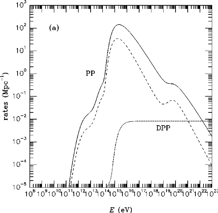
Figure 5: The relevant interaction rates at $z=0$ that affect the photons and electrons in the energy range we consider. The key is identical to the key for Fig. 4. The rates are calculated by folding the total cross sections and inelasticity weighted cross sections with the present background photon spectrum shown in Fig 2.

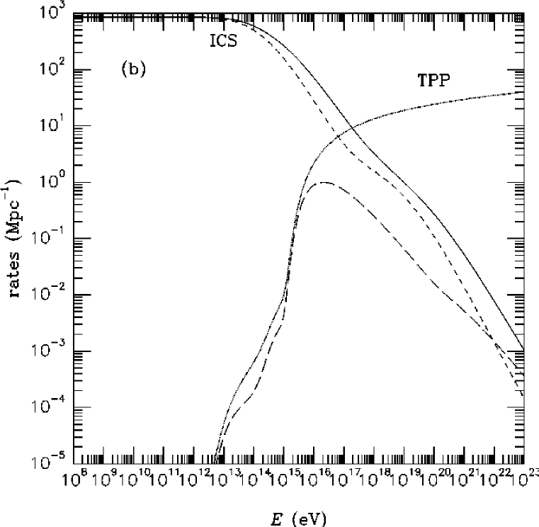
Figure 5: (b).

In Fig. 4(b) we plot $\sigma(s)$ and $\sigma(s)\eta(s)$ of which the latter is proportional to the fractional energy loss rate of the “leading particle”, for ICS and TPP. Fig. 5 shows all the rates at redshift $z=0$ that affect the photons and electrons in the energy range we consider.

3.1.5 Other Processes

Other interactions that are neglected in this paper are all processes involving the productions of one or more $e^{-}e^{+}$ pairs substituted by muon, tau lepton, and pion pairs, double Compton scattering ($e\gamma_{b}\rightarrow e\gamma\gamma$), $\gamma\gamma$ scattering ($\gamma\gamma_{b}\rightarrow\gamma\gamma$), Bethe-Heitler pair production ($\gamma X\rightarrow Xe^{+}e^{-}$, where $X$ can be an atom, an ion, or a free electron), the process $\gamma\gamma_{b}\rightarrow e^{+}e^{-}\gamma$, and pair production on a magnetic field ($\gamma B\rightarrow e^{-}e^{+}$). The total cross section of single muon pair production ($\gamma\gamma_{b}\rightarrow\mu^{-}\mu^{+}$), for example, is smaller than electron pair production by about a factor of 10. Energy loss rates for TPP involving heavier pairs are suppressed by a factor $\simeq(m/m_{e})^{1/2}$ in the limit of large $s$. Similarly, double pair production involving heavier pairs is also negligible [74]. The double Compton scattering cross section is of order $\alpha^{3}$ and must be treated together with the radiative corrections to ordinary Compton scattering of the same order. The corrections to the lowest order ICS cross section by processes involving $m_{\gamma}$ additional photons in the final state, $e\gamma_{b}\rightarrow e+(m_{\gamma}+1)\gamma$, $m_{\gamma}\geq 1$, turn out to be less than 10% in the energy range under consideration [80]. A similar remark applies to corrections to the lowest order PP cross section by the processes $\gamma\gamma_{b}\rightarrow e^{+}e^{-}+m_{\gamma}\gamma$, $m_{\gamma}\geq 1$. Photon-photon scattering can only play a role for $z\mathrel{\mathchoice{\lower 3.6pt\vbox{\halign{$\mathsurround=0pt\displaystyle\hfil#\hfil$\cr>\crcr\sim\crcr}}}{\lower 3.6pt\vbox{\halign{$\mathsurround=0pt\textstyle\hfil#\hfil$\cr>\crcr\sim\crcr}}}{\lower 3.6pt\vbox{\halign{$\mathsurround=0pt\scriptstyle\hfil#\hfil$\cr>\crcr\sim\crcr}}}{\lower 3.6pt\vbox{\halign{$\mathsurround=0pt\scriptscriptstyle\hfil#\hfil$\cr>\crcr\sim\crcr}}}}100$ and energies below the redshift dependent pair production threshold Eq. (1) [81, 82]. A similar remark applies to Bethe-Heitler pair production on atoms, ions and free electrons [82]. Pair production on a magnetic field of order $10^{-6}{\,{\rm G}}$ which is typical for the field of Our Galaxy, is only relevant for $E\mathrel{\mathchoice{\lower 3.6pt\vbox{\halign{$\mathsurround=0pt\displaystyle\hfil#\hfil$\cr>\crcr\sim\crcr}}}{\lower 3.6pt\vbox{\halign{$\mathsurround=0pt\textstyle\hfil#\hfil$\cr>\crcr\sim\crcr}}}{\lower 3.6pt\vbox{\halign{$\mathsurround=0pt\scriptstyle\hfil#\hfil$\cr>\crcr\sim\crcr}}}{\lower 3.6pt\vbox{\halign{$\mathsurround=0pt\scriptscriptstyle\hfil#\hfil$\cr>\crcr\sim\crcr}}}}10^{24}{\,{\rm eV}}$. This critical energy is even higher for the EGMF and this process is thus negligible in the analysis.

3.2 Nucleons

There are three major processes that affect the propagation of protons and neutrons: Electron-positron pair production by protons (PPP; $p\gamma_{b}\rightarrow pe^{-}e^{+}$), photopion production ($N\gamma_{b}\rightarrow N(n\pi),n\geq 1$), and neutron $\beta$-decay ($n\rightarrow pe^{-}\bar{\nu}_{e}$).

3.2.1 Pair Production by Protons

PPP provides the main energy attenuation for protons with energies below the GZK cutoff [83]. The energy threshold for this process is

$$E_{\rm th}=\frac{m_{e}(m_{N}+m_{e})}{\epsilon}\simeq 4.8\times 10^{14}\left(\frac{\epsilon}{{\,{\rm eV}}}\right)^{-1}{\,{\rm eV}}.$$ (28)

Thus, for a microwave background photon ($\epsilon\sim 10^{-3}{\,{\rm eV}}$), PPP ensues at a proton energy $E\sim 5\times 10^{17}{\,{\rm eV}}$. Below this energy, the protons cool essentially only by redshifting with the expansion.

The PPP total cross section behaves very similarly to that for triplet pair production because PPP is almost identical to TPP [84], and the expression for the total cross section away from the threshold may be given by Eq. (24). However, while TPP near its threshold is dominated by other processes, the exact behavior of PPP rates near the threshold are very important because PPP dominates the proton energy loss in that energy range. I use the parametric fits given in Ref. [85] for the cross section and inelasticity. Then I use the same approach in calculating the differential rates as we did for TPP. It can be shown that these rates are well approximated by a power law. On the other hand, the proton spectrum evolution due to PPP is well described by CEL because the inelasticities are smaller than $10^{-3}$ at all relevant energies. Production of heavier pairs like $\mu^{+}\mu^{-}$ is suppressed similarly to the case of TPP. The energy ranges for the produced pairs and the recoiling proton are given in Appendix A.

3.2.2 Photopion Production

Photopion production provides the main energy attenuation for nucleons above $E\simeq 10^{19}{\,{\rm eV}}$. The energy threshold for this process is

$$E_{\rm th}=\frac{m_{N}m_{\pi}+m^{2}_{\pi}/2}{\epsilon}\simeq 6.8\times 10^{16}\left(\frac{\epsilon}{{\,{\rm eV}}}\right)^{-1}{\,{\rm eV}}.$$ (29)

Thus, for a microwave background photon ($\epsilon\sim 10^{-3}{\,{\rm eV}}$), photopion production ensues at a nucleon energy $E\sim 7\times 10^{19}{\,{\rm eV}}$. Since publications on numerical studies of nucleon and $\gamma$-ray propagation usually do not contain detailed information on the implementation especially of multiple pion production, I present our approach here in some detail. First, I define a few suitable kinematic variables which depend only on the incoming particles. If $E_{\gamma}^{\rm lab}$ is the photon energy in the laboratory frame (LF) where the nucleon is at rest, $m_{N}$ is the nucleon mass, and $s$ is the squared center of mass (CM) energy, then the following relations hold:

$$\kappa \equiv \frac{E_{\gamma}^{\rm lab}}{m_{N}}=\frac{\epsilon E_{N}}{m_{N}^{2}}(1-\mu)\,,$$

$$s = m_{N}^{2}(1+2\kappa)\,.$$ (30)

Since laboratory measurements of cross sections are usually given in terms of $E_{\gamma}^{\rm lab}$, I will conveniently express everything in terms of $\kappa$ in the following.

Concerning single pion production I consider the following reactions:

$$\gamma+N \rightarrow \pi^{0}+N\,:\,{d\sigma_{1}\over d\Omega^{*}}=\sum_{j=0}^{K}a_{1j}(\kappa)\left(x^{*}\right)^{j}\,,$$ (31)

$$\gamma+p \rightarrow \pi^{+}+n\,:\,{d\sigma_{2}\over d\Omega^{*}}=\left(1-\beta^{*}x^{*}\right)^{-1/2}\sum_{j=0}^{K}a_{2j}(\kappa)\left(x^{*}\right)^{j}\,,$$ (32)

$$\gamma+n \rightarrow \pi^{-}+p\,:\,{d\sigma_{3}\over d\Omega^{*}}=\left(1-\beta^{*}x^{*}\right)^{-1/2}\sum_{j=0}^{K}a_{3j}(\kappa)\left(x^{*}\right)^{j}\,.$$ (33)

The differential cross sections for these processes are expressed here in terms of $\kappa$ and the CM quantities $\Omega^{*}$, $\beta^{*}$, and $x^{*}$ which denote solid angle, pion velocity, and the cosine of the scattering angle, respectively. The functions $a_{ij}(\kappa)$, $i=1,2,3$ and $j=1,\cdots,N$ are fitted to laboratory cross section data and I use fits up to order $K=3$ [86]. The expressions in Eqs. (31)-(33) can be easily rewritten in terms of the energies of the outgoing nucleons and pions in the cosmic ray frame (CRF) which I denote by $E^{\prime}_{a}$ for $a=p,n,\pi^{+},\pi^{-},\pi^{0}$. The relevant formulae are be given in Appendix B.

Note that in Eq. (31) I have assumed identical cross sections for the two charge retention processes involving protons and neutrons. This is a very good approximation (see, e.g. Ref. [86]). Reactions (32) and (33) constitute the charge exchange reactions for single pion production.

We now turn to multiple pion production. Let us first consider the channel $\gamma+p\rightarrow\pi^{-}+X$ where $X$ stands for anything. This channel has been discussed in detail in Ref. [87]. There, the Feynman $x$-variable $x=p_{\|}^{*}/p_{\rm max}^{*}$ was introduced, which is the fraction of the pion parallel momentum $p_{\|}^{*}$ in the CMF to its maximal value

$$p_{\rm max}^{*}=m_{N}\frac{D}{(1+2\kappa)^{1/2}}\,,$$ (34)

where $D\equiv[(\kappa-\varepsilon^{2}/2)^{2}-\varepsilon^{2}]^{1/2}$, and $\varepsilon=m_{\pi}/m_{N}$ is the ratio of the pion and nucleon mass. Denoting the transverse momentum with $p_{\bot}$ and the $\pi^{-}$ energy in the CMF by $E_{\pi^{-}}^{*}$, the differential cross section for $\pi^{-}$ production was written in terms of a structure function $f(x,p_{\bot}^{2},s)$:

$$d^{2}\sigma_{\gamma p\rightarrow\pi^{-}X}=\pi\,{p_{\rm max}^{*}\over E_{\pi^{-}}^{*}}\,f(x,p_{\bot}^{2},s)\,dx\,dp_{\bot}^{2}\,.$$ (35)

Performing Lorentz transformations into the CRF where the proton and $\pi^{-}$ energies are $E_{p}$ and $E^{\prime}_{\pi^{-}}$ (see Appendix B), this can be written as

$${d\sigma_{\gamma p\rightarrow\pi^{-}X}\over dE^{\prime}_{\pi^{-}}} = {2\pi m_{N}p_{\rm max}^{*}\over E_{p}}\left(1+2\kappa\right)^{1/2}\int_{x_{\rm min}}^{x_{\rm max}}dx$$

$$\times f\left[x,-m_{\pi}^{2}+\left({E^{\prime}_{\pi^{-}}m_{N}\over E_{N}}\right)^{2}(1+2\kappa)+2p_{\rm max}^{*}\left({E^{\prime}_{\pi^{-}}m_{N}\over E_{N}}\right)(1+2\kappa)^{1/2}x,s\right]\,,$$

where $x_{\rm min}\geq-1$ is chosen such that $p_{\bot}^{2}\geq 0$ which is the second argument of $f$, and $x_{\rm max}$ such that $p_{\bot}^{2}/(p_{\rm max}^{*})^{2}+x^{2}\leq 1$.

For $s\rightarrow\infty$ the structure function $f$ is independent of $s$ [87, 88]. I will therefore neglect any $s$-dependence altogether. Furthermore, I take into account these processes only above some threshold which is sufficiently high such that the contribution of single pion production is negligible; I take $\kappa\geq 2(\varepsilon+\varepsilon^{2})$.

Finally, for our purposes I assume that the remaining dependence of $f(x,p_{\bot}^{2})$ factorizes into an $x$-dependent part and an exponential dependence on $p_{\bot}^{2}$:

$$f(x,p_{\bot}^{2},s)\simeq{1\over\Lambda^{2}}\ \exp[-p_{\bot}^{2}/\Lambda^{2}]\,f(x)\,.$$ (37)

Here, $\Lambda\simeq{\rm GeV}/6.4$ is roughly of the order of the QCD scale and $f(x)$ can be fitted to the data presented in Ref. [87].

Within these approximations we have finally

$${d\sigma_{4}\over dE^{\prime}_{\pi^{-}}} \equiv {d\sigma_{\gamma p\rightarrow\pi^{-}X}\over dE^{\prime}_{\pi^{-}}}={2\pi\over E_{p}}\left({m_{N}\over\Lambda}\right)^{2}D\int_{x_{\rm min}}^{x_{\rm max}}dxf(x)$$

$$\times\exp\left\{-\left({m_{N}\over\Lambda}\right)^{2}\left[-\varepsilon^{2}+\left({E^{\prime}_{\pi^{-}}\over E_{p}}\right)^{2}(1+2\kappa)+2D\left({E^{\prime}_{\pi^{-}}\over E_{p}}\right)x\right]\right\}\,,$$

where $x_{\rm min}$ and $x_{\rm max}$ are given by

$$x_{\rm min} = \max\left[-1,\frac{\varepsilon^{2}-(E^{\prime}_{\pi^{-}}/E_{p})^{2}(1+2\kappa)}{2D(E^{\prime}_{\pi^{-}}/E_{p})}\right]\,,$$

$$x_{\rm max} = -\frac{E^{\prime}_{\pi}}{E_{p}}\frac{1+2\kappa}{D}+\left(1+\varepsilon^{2}\frac{1+2\kappa}{D^{2}}\right)^{1/2}\,.$$ (39)

At this point it is important to realize that $f(x)=f_{c}(x)+f_{\rho}(x)$ can be divided into a contribution $f_{c}(x)$ from the “central” pions and a contribution $f_{\rho}(x)$ from production of multiple $\rho_{0}$ mesons (sometimes also called the leading pion contribution) which subsequently decay into equal distributions of $\pi^{+}$ and $\pi^{-}$. Therefore, $f_{\rho}(x)$ exclusively contributes to the production of $\pi^{+}$ and $\pi^{-}$ and corresponds to a charge retention process where the nature of the nucleon is unchanged. In contrast, $f_{c}(x)$ describes a process resulting in approximately equal distributions of $\pi^{0}$ and $\pi^{-}$ with the probability for change of nucleon isospin being about $2/5$ (from simple quark counting).

From these assumptions it follows immediately that $d\sigma_{5}/dE^{\prime}_{\pi^{0}}\equiv d\sigma_{\gamma p\rightarrow\pi^{0}X}/dE^{\prime}_{\pi^{0}}$ is obtained by substituting $f_{c}(x)$ for $f(x)$ in Eq. (3.2.2).

In addition, I assume that inclusive and leading pion production takes place with the approximately constant cross sections $\sigma_{\rm tot}\simeq 127$ $\mu{\rm b}$ and $\sigma_{\rho}\simeq 21.5$ $\mu{\rm b}$, respectively. We can then define the average central $\pi^{-}$ multiplicity by

$$\left\langle n_{\pi^{-}}^{c}\right\rangle(\kappa)={\pi\over\sigma_{\rm tot}}\int dp_{\bot}^{2}\int dxf_{c}(x){\exp[-p_{\bot}^{2}/\Lambda^{2}]\over\Lambda^{2}}\left[x^{2}+{1+2\kappa\over D^{2}}\left({p_{\bot}^{2}\over m_{N}^{2}}+\varepsilon^{2}\right)\right]^{-1/2}\,.$$ (40)

The integration range is determined by $p_{\bot}^{2}/(p_{\rm max}^{*})^{2}+x^{2}\leq 1$. By evaluating this formula one can see that the multiplicity $\left\langle n_{\pi^{-}}^{c}\right\rangle$ increases asymptotically logarithmically in $s$ for $s\rightarrow\infty$. Applying charge conservation to the central pion distribution, making the above assumptions and in addition assuming $\pi^{+}$ and $\pi^{-}$ distributions to be proportional to each other uniquely determines $d\sigma_{6}/dE^{\prime}_{\pi^{+}}\equiv d\sigma_{\gamma p\rightarrow\pi^{+}X}/dE^{\prime}_{\pi^{+}}$. It is obtained by substituting $\left[1+(2/5)(1-\sigma_{\rho}/\sigma_{\rm tot})/\left\langle n_{\pi^{-}}^{c}\right\rangle(\kappa)\right]f_{c}(x)+f_{\rho}(x)$ for $f(x)$ in Eq. (3.2.2).

It is now easy to compute the fractions $r_{c}(\kappa)$ and $r_{\rho}(\kappa)$ of the incoming nucleon energy which go into the central and leading pions, respectively (see Appendix B). Fig. 6 shows these fractions and the central and total $\pi^{-}$ multiplicities as functions of $s$. Assuming a flat distribution for the outgoing nucleons, we then have

$${d\sigma_{p\rightarrow p}\over dE^{\prime}_{p}} = {\sigma_{\rho}\over 2r_{\rho}(\kappa)E_{p}}\,\Theta\left[{E^{\prime}_{p}\over E_{p}}-1+2r_{\rho}(\kappa)\right]+{3\over 5}\,{\sigma_{\rm tot}-\sigma_{\rho}\over 2r_{c}(\kappa)E_{p}}\,\Theta\left[{E^{\prime}_{p}\over E_{p}}-1+2r_{c}(\kappa)\right]\,,$$

$${d\sigma_{p\rightarrow n}\over dE^{\prime}_{n}} = {2\over 5}\,{\sigma_{\rm tot}-\sigma_{\rho}\over 2r_{c}(\kappa)E_{p}}\,\Theta\left[{E^{\prime}_{n}\over E_{p}}-1+2r_{c}(\kappa)\right]$$ (41)

for the charge retention and charge exchange cross sections, respectively. For the processes involving an incoming neutron, I assume that the cross sections are also given by the above expressions after substituting $p\leftrightarrow n$ and $\pi^{+}\leftrightarrow\pi^{-}$ everywhere. Fig. 7 shows the differential cross sections for production of $\pi^{-}$, $\pi^{+}$, $\pi^{0}$, protons, and neutrons for an incoming proton for two different CM energies resulting from the formalism adopted above. Fig. 8 shows the inclusive pion production cross sections for nucleons as a function of $s$. Fig. 9 shows all the rates at redshift $z=0$ that affect the nucleons in the energy range we consider.

Pions produced by nucleons quickly decay to EM particles and neutrinos and feed the EM cascade. $\pi^{0}$ decays into photons ($\pi^{0}\rightarrow\gamma\gamma$), and $\pi^{\pm}$ decays to produce electrons, positrons, and neutrinos ($\pi^{\pm}\rightarrow\mu^{\pm}\nu_{\mu}(\bar{\nu}_{\mu});\mu^{\pm}\rightarrow e^{\pm}\nu_{e}(\bar{\nu}_{e})\bar{\nu}_{\mu}(\nu_{\mu})$) [89]. Since the decay time of pions is very short compared to the timescale in the problem, I assume that pions are converted into secondary particles instantaneously. The decay spectra of the secondary particles may be calculated easily [20]. The expressions for the decay spectra are given in Appendix C.

3.2.3 Neutron $\beta$-decay

Below $\sim 10^{20}{\,{\rm eV}}$, neutron $\beta$-decay is the fastest process among the interactions that affect nucleons in the problem. The neutron decay rate is $\Gamma=\Gamma_{0}/\gamma_{n}=1/\tau_{n}\gamma_{n}$, where $\tau_{n}$ is the neutron lifetime ($\tau_{n}\simeq 888.6\pm 3.5$ sec), and $\gamma_{n}$ is the neutron Lorentz factor. The range $R_{n}$ of a neutron is given as

$$R_{n}\simeq\frac{c}{\Gamma}=c\tau_{n}\gamma_{n}\simeq 0.9\left(\frac{E_{n}}{10^{20}{\,{\rm eV}}}\right){\,{\rm Mpc}}.$$ (42)

In calculating the spectrum of secondary particles, I neglect the proton kinetic energy in the neutron rest frame, as is usually done. The result can be found in standard textbooks such as Ref. [90].

Fig. 10 shows the energy attenuation lengths for cascade photons and nucleons as functions of energy in the CEL approximation.

4 Comparison with other Work

Before I apply the propagation code to specific HECR injection scenarios in the next section, I compare the predicted spectra with results from other investigations for some standard situations. For a discrete source producing a differential injection spectrum $F_{a}(E)$ of particle type $a$ (in units of number per energy per time) at redshift $z=z_{i}$, we obtain the spectrum $j_{a}(E)$ (in units of number per area per time per solid angle per energy) observed at $z=0$ in the following way: I impose the boundary condition

$$N_{a}(E,z_{i})={(1+z_{i})^{2}\over r_{i}^{2}}F_{a}(E)\,,$$ (43)

where $r_{i}$ is the comoving dimensionful source distance corresponding to redshift $z_{i}$ ($r_{i}=2H_{0}^{-1}[1-(1+z_{i})^{-1/2}]$ in our cosmology), and solve the propagation equations for vanishing source terms. If we denote the resulting distribution at $z=0$ by $N_{a}(E)$, then $j_{a}(E)=N_{a}(E)/(4\pi)$ and the modification factor $M_{a}(E,z_{i})$, defined as in Ref. [42, 44], is given by

$$M_{a}(E,z_{i})\equiv{4\pi d_{L}^{2}j_{a}(E)\over F_{a}(E)}=(1+z_{i})^{4}{N_{a}(E)\over N_{a}(E,z_{i})}\,,$$ (44)

where I used the luminosity distance $d_{L}\equiv r_{i}(1+z_{i})$ [91].

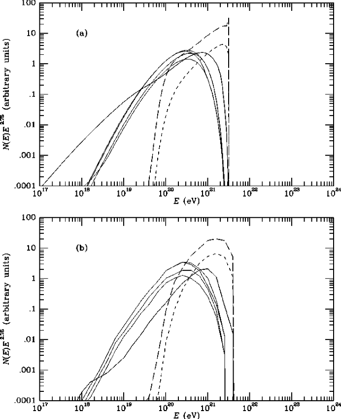
Figure 12: The differential fluxes of $\gamma$-rays (solid line), nucleons (long dashed line), neutrons (short dashed line) and $\nu_{\mu}$, $\bar{\nu}_{\mu}$, $\nu_{e}$, $\bar{\nu}_{e}$ (thin solid lines in decreasing order) for monoenergetic proton injection at an energy $E=10^{21.5}{\,{\rm eV}}$ and a distance $d=32{\,{\rm Mpc}}$: (a) Result from our analysis in arbitrary units; (b) Corresponding results from Ref. [51].

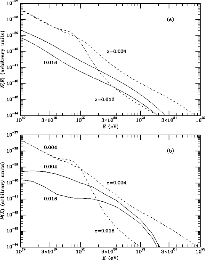
Figure 13: The differential fluxes of $\gamma$-rays (solid lines) and nucleons (long dashed lines) from a discrete source injecting a $E^{-2}$ proton spectrum extending up to $10^{22}{\,{\rm eV}}$, located at the redshift indicated: (a) Result from our analysis in arbitrary units; (b) Corresponding results from Ref. [47].

In Fig. 11 I plot the modification factors as defined in Ref. [44] for discrete sources injecting protons with a power law at a given distance along with the corresponding curves from Ref. [51]. It can be seen that our results lie somewhat between results from Refs. [51] and [47]. In Fig. 12 I compare the nucleon, $\gamma$-ray and neutrino fluxes computed for monoenergetic proton injection at a given distance with results from Ref. [51]. In our prediction the secondary $\gamma$-ray flux at the low energy side is higher than the one given in Ref. [51] by a factor $\simeq 10$. I attribute that to the fact that the differential multiple pion production cross section used in our analysis (see Fig. 7) peaks at low energies. In Fig. 13 I consider the case of power law injection by a single source and compare the nucleon and $\gamma$-ray fluxes with corresponding results in Ref. [47]. The nucleon fluxes agree well, whereas, again, our prediction for the $\gamma$-ray flux is higher at the low energy side and lower at the high energy side. Since Refs. [47, 51] do not give detailed information on their treatment of pion production, it is hard to give an exhaustive explanation of these differences. This, however, will not have an influence on our considerations where secondary $\gamma$-ray production by nucleons plays a minor role.

5 Application to Models of HECR Origin

We are now in a position to compute the cosmic and $\gamma$-ray fluxes predicted by various models of HECR origin. Since there is currently no unambiguous information on HECR composition, I will normalize the predicted sum of $\gamma$-ray and nucleon fluxes to the observed HECR flux. This is done to optimally enable an explanation for the events above $10^{20}{\,{\rm eV}}$ without overshooting the UHE flux at lower energies (which might be explained by more conventional components) or predicting an excessive integral flux above $10^{20}{\,{\rm eV}}$. I estimate the uncertainty in the predicted $\gamma$-ray flux at lower energies induced by this normalization procedure to be less than a factor $\simeq 3$.

5.1 GUT Scale Physics Models

As already mentioned in the introduction, it has been suggested that HECRs may have a nonacceleration origin [27, 28, 29, 30, 31, 32, 33, 34] such as the decay of supermassive elementary “X” particles associated with Grand Unified Theories (GUTs), for example. These particles could be radiated from topological defects (TDs) formed in the early universe during phase transitions caused by spontaneous breaking of symmetries implemented in these GUTs (for a review on TDs, see [92]). This is because TDs, such as ordinary and superconducting cosmic strings, domain walls and magnetic monopoles, are topologically stable but nevertheless can release part of their energy in the form of these X particles due to physical processes like collapse or annihilation. The corresponding injection rate of X particles $dn_{X}/dt$ as a function of cosmic time $t$ is usually parametrized as

$${dn_{X}\over dt}\propto t^{-4+p}\,,$$ (45)

where $p\geq 0$ depends on the evolution of TDs. For example, X particle release from a network of ordinary cosmic strings in the scaling regime would correspond to $p=1$ if one assumes that a constant fraction of the total energy in closed loops goes into X particles [29, 31]. Annihilation of magnetic monopoles and antimonopoles [27, 33] predicts $p=1$ in the matter dominated and $p=3/2$ in the radiation dominated era [56] whereas the simplest models for superconducting cosmic strings lead to $p=0$ [28]. A constant comoving injection rate corresponds to $p=2$ and $p=5/2$ during the matter and radiation dominated era, respectively.

The X particles with typical GUT scale masses $m_{X}$ of the order of $10^{16}{\,{\rm GeV}}$ subsequently decay into leptons and quarks. The strongly interacting quarks fragment into a jet of hadrons which results in mesons and baryons that are typically of the order of $10^{4}-10^{5}$. It is assumed that these hadrons then give rise to a substantial fraction of the HECR flux as well as a considerable neutrino flux.

The shapes of the nucleon and $\gamma$-ray spectra predicted within such TD models are thus expected to be universal (i.e., independent of the specific process involving any specific kind of TD) at ultrahigh energies and to be dependent only on the physics of X particle decay. This is because at HECR energies nucleons and $\gamma$-rays have attenuation lengths in the cosmic microwave background (CMB) which are small compared to the Hubble scale. Cosmological evolutionary effects which depend on the specific TD model and are usually parametrized by Eq. (45) are therefore negligible. In contrast, the predicted neutrino flux and the $\gamma$-ray flux below the pair production threshold on the CMB [see Eq. (1)] depend on the energy release integrated over redshift and thus on the specific TD model.

I now discuss the particular form of the particle injection spectra expected from X particle release. I assume that each X-particle decays into a lepton and a quark each of an energy approximately half of the X particle mass $m_{X}$. For reasonable extragalactic field strengths, the lepton (which I assume to be an electron in the following) will quickly be degraded by synchrotron loss producing synchrotron photons of a typical energy given by Eq. (8). This energy is typically much smaller than $10^{20}{\,{\rm eV}}$ where the resulting contribution to the $\gamma$-ray flux is likely to be buried below the charged CR flux. For that reason, the GUT-scale lepton was usually omitted. However, for high EGMF strengths the synchrotron peak can approach $10^{20}{\,{\rm eV}}$ and thus could become relevant. For the present analysis I will thus include the source term for the GUT-scale lepton by writing its injection flux at energy $E$ and time $t$ as

$$\Phi_{e}(E,t)={dn_{X}(t)\over dt}\,\delta(E-m_{X}/2)\,,$$ (46)

in units of particles per volume per time per energy.

The quark from X particle decay hadronizes by jet fragmentation and produces nucleons, $\gamma$-rays and neutrinos, the latter two from the decay of neutral and charged pions in the hadronic jets. The hadronic route is expected to produce the largest number of particles. The resulting effective injection spectrum for particle species $a$ from the hadronic channel can be written as

$$\Phi_{a}(E,t)={dn_{X}(t)\over dt}{2\over m_{X}}{dN_{a}(x)\over dx}\,,$$ (47)

where $x\equiv 2E/m_{X}$, and $dN_{a}/dx$ is the effective fragmentation function describing the production of the particles of species $a$ from the original quark.

The spectra of the hadrons in a jet produced by the quark are, in principle, given by quantum chromodynamics (QCD). Suitably parametrized QCD motivated hadronic spectra that fit well the data in collider experiments in the GeV–TeV energies have been suggested in the literature [27]. The total hadronic fragmentation spectrum $dN_{h}/dx$ is taken to be of the form [27]

$${dN_{h}(x)\over dx}=\left\{\begin{array}[]{ll}{15\over 16}x^{-1.5}(1-x)^{2}&\mbox{if $x_{0}\leq x\leq 1$}\\ 0&\mbox{otherwise}\end{array}\right.\,,$$ (48)

where the lower cutoff $x_{0}$ is typically taken to correspond to a cut-off energy $\sim 1{\,{\rm GeV}}$. The spectrum Eq. (48) obeys energy conservation, $\int_{x_{0}}^{1}dxx(dN_{h}(x)/dx)=1$. Assuming a nucleon content of $\simeq 3\%$ and the rest equally distributed among the three types of pions, we can write the fragmentation spectra as [32, 50]

$${dN_{N}(x)\over dx} = (0.03)\,{dN_{h}(x)\over dx}\,,$$ (49)

$${dN_{\pi^{+}}\over dx} = {dN_{\pi^{-}}\over dx}={dN_{\pi^{0}}\over dx}=\left({0.97\over 3}\right){dN_{h}(x)\over dx}\,.$$

From the pion injection spectra one gets the resulting contribution to the injection spectra for $\gamma$-rays, electrons and neutrinos by applying the formulae in Appendix C.

Independently of the spectral shapes of the predicted nucleon and $\gamma$-ray fluxes, the question for the absolute normalization of the injection rates $dn_{X}/dt$ in Eqs. (45), (46) and (47) arises. It has been shown, for example for cosmic strings [29, 31] and annihilation of magnetic monopoles and antimonopoles [33], that at least some TD models are capable of producing an observable HECR flux if reasonable parameters are adopted. For the purposes of this paper I will therefore not consider this issue and simply adopt the normalization procedure mentioned above.

TD models of HECR origin are subject to a variety of constraints mostly of cosmological nature. These are mainly due to the comparatively substantial predicted energy injection at high redshift [see Eq. (45)]. Note that more conventional CR sources like galaxies start to inject energy only at a redshift of a few. Using an analytical approximation for the cascade spectrum below the pair production threshold on the CMB resulting from X particle injection, one can derive constraints from cascading nucleosynthesis and light element abundances, CMB distortions, and the measured $\gamma$-ray background [59, 58, 60] in the $100{\,{\rm MeV}}$ region [56], as well as from observational limits on the $\gamma$-ray to charged CR flux ratio between $10^{13}{\,{\rm eV}}$ and $10^{14}{\,{\rm eV}}$ [93, 34]. The $100{\,{\rm MeV}}$ $\gamma$-ray background constraint was first discussed in Refs. [49, 55]. In the context of top-down models it was applied in Refs. [94, 95] on the basis of analytical approximations.

In addition, there has been a claim recently [51] that TD models might be ruled out altogether due to overproduction of $\gamma$-rays in the range between the knee and $\sim 10^{19}{\,{\rm eV}}$. This would occur for EGMFs stronger than about $10^{-10}{\,{\rm G}}$ due to synchrotron radiation from the electronic component of the TD induced flux which was normalized to the observed flux at $3\times 10^{20}{\,{\rm eV}}$. However, in my opinion, the argument in Ref. [51] suffers from several shortcomings: First, monoenergetic injection of protons and $\gamma$-rays was used instead of the more realistic injection spectra such as the ones discussed above in Eqs. (48) and (49). And second, only the case of a single, discrete TD source at a fixed distance from the observer was considered instead of more realistic source distributions and evolution histories. Finally, electron deflection due to the EGMF which can influence the processed spectrum from a single source was neglected. Nevertheless, I simulated the situation of Fig. 13 in Ref. [51] for an EGMF of $10^{-9}{\,{\rm G}}$ on which their claim is based. As a result I got a spectrum whose shape is roughly similar to Fig. 13 in Ref. [51], but the details of the spectrum differed somewhat, part of which can be attributed to a different model of the radiation background. The synchrotron peak I got was about an order of magnitude lower than in Ref. [51] relative to other parts of the spectrum. Most importantly, however, we observe that if the spectrum is normalized to the highest energy event this model would predict simply too many events above $10^{20}\,$eV including the original injection peak. Therefore, the model adopted in Ref. [51] is not a realistic model for UHE CRs to start with. I thus conclude that it is not possible to rule out TD models on the basis of the discussion in Ref. [51].

Our goal here is to reexamine the constraints based on the predicted $\gamma$-ray flux in the regimes around $100{\,{\rm MeV}}$, between $10^{13}{\,{\rm eV}}$ and $10^{14}{\,{\rm eV}}$, and between the knee and $10^{19}{\,{\rm eV}}$, using our numerical techniques discussed in the previous section, I base this on realistic injection spectra and histories as discussed above. To my knowledge, this has not been done yet despite its importance for making $\gamma$-ray flux based constraints more reliable.

The redshift range of energy injection contributing to the $\gamma$-ray flux at energy $E_{\gamma}$ today is given by $1+z\mathrel{\mathchoice{\lower 3.6pt\vbox{\halign{$\mathsurround=0pt\displaystyle\hfil#\hfil$\cr<\crcr\sim\crcr}}}{\lower 3.6pt\vbox{\halign{$\mathsurround=0pt\textstyle\hfil#\hfil$\cr<\crcr\sim\crcr}}}{\lower 3.6pt\vbox{\halign{$\mathsurround=0pt\scriptstyle\hfil#\hfil$\cr<\crcr\sim\crcr}}}{\lower 3.6pt\vbox{\halign{$\mathsurround=0pt\scriptscriptstyle\hfil#\hfil$\cr<\crcr\sim\crcr}}}}\left(E_{\rm th}(z=0)/E_{\gamma}\right)^{1/2}$ where $E_{\rm th}(z=0)$ is the PP threshold on the CMB at $z=0$ [see Eq. (1)]. Since our interest is in the $\gamma$-ray flux at $E_{\gamma}\mathrel{\mathchoice{\lower 3.6pt\vbox{\halign{$\mathsurround=0pt\displaystyle\hfil#\hfil$\cr>\crcr\sim\crcr}}}{\lower 3.6pt\vbox{\halign{$\mathsurround=0pt\textstyle\hfil#\hfil$\cr>\crcr\sim\crcr}}}{\lower 3.6pt\vbox{\halign{$\mathsurround=0pt\scriptstyle\hfil#\hfil$\cr>\crcr\sim\crcr}}}{\lower 3.6pt\vbox{\halign{$\mathsurround=0pt\scriptscriptstyle\hfil#\hfil$\cr>\crcr\sim\crcr}}}}100{\,{\rm MeV}}$, I maximally integrate up to $1+z_{\rm max}=10^{3}$. The spectrum in this energy range converges before we reach this redshift. A word of caution is in order for the predicted neutrino spectra. The UHE neutrinos interact with the universal neutrino background with $T_{\nu}\sim 1.95\,$K, and produce $l\bar{l}$ where $l=e,\mu,\tau,\nu,q,\ldots$ via $Z_{0}$ resonance [32, 40]. The decay products of $\mu,\tau,q$ contain secondary neutrinos. Here I consider only simple absorption of UHE neutrinos, i.e. I integrate up to the average absorption redshift $z_{\rm abs}$ due to this interaction [32]. The neutrino spectra also converge rather fast with increasing redshift for the parameters I used for TD models. Furthermore, the modification to the neutrino spectra due to the cascading by the aforementioned interaction is expected to be small for these parameters [40]. Therefore, the neutrino spectra given in this paper are expected to be good approximations to the real converged spectra. I leave a more detailed calculation of the UHE neutrino flux to future work.

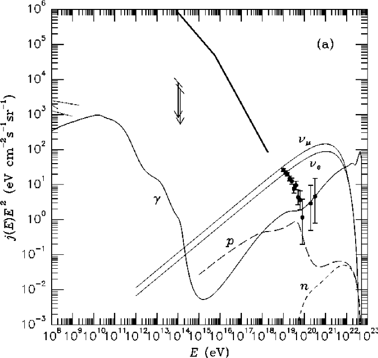
Figure 14: Predictions for the differential fluxes of $\gamma$-rays (solid line), protons (long dashed line), neutrons (short dashed line), and $\nu_{\mu}(\bar{\nu}_{\mu}),\nu_{e}(\bar{\nu}_{e})$ (thin solid lines in decreasing order) by a typical topological defect scenario for a vanishing EGMF. This model assumes uniform injection rates with spectra given by Eq. (46) and (47) for the QCD motivated fragmentation functions Eq. (48) and (49) for $m_{X}=10^{23}{\,{\rm eV}}$. The injection history is given by Eq. (45) for: (a) $p=1$. Also shown are the combined data from the Fly’s Eye [8, 9] and the AGASA [11, 12] experiments above $10^{19}{\,{\rm eV}}$ (dots with error bars), piecewise power law fits to the charged CR flux (thick solid line) and observational upper limits on the $\gamma$-ray flux around $100{\,{\rm MeV}}$ from Refs. [58, 59, 60] (dotted lines in decreasing order). The arrows indicate the limits on the $\gamma$-ray to charged CR flux ratio from Ref. [93].

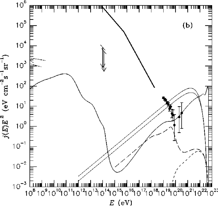
Figure 14: (b) $p=2$.

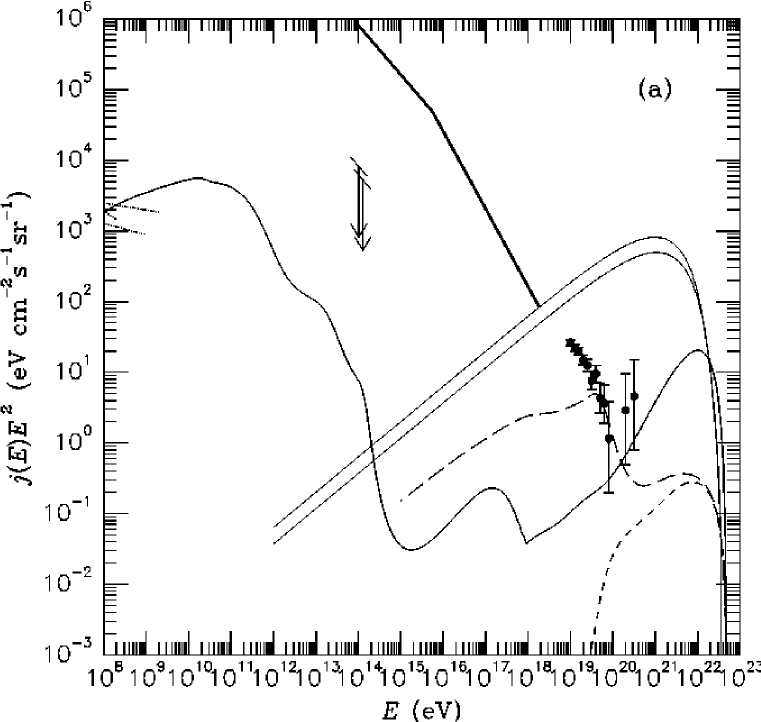
Figure 16: (a) Same as Fig. 14(a), but for an EGMF of $10^{-9}\,$G.

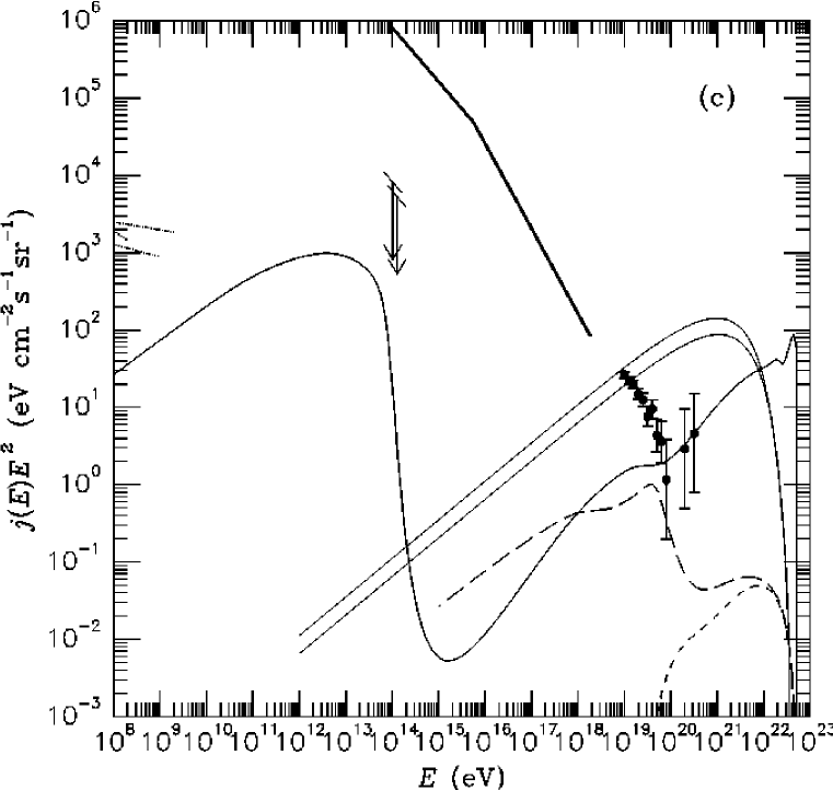
Figure 16: (c) Same as Fig. 14(a), but assuming absence of any IR/O background. These panels demonstrate the EGMF and IR/O background dependence of the predicted HECR flux shape and composition and its influence on the prediction for the $\gamma$-ray background at lower energies.

I performed simulations assuming uniform injection rates given by Eqs. (46)-(49) for $m_{X}=10^{23}{\,{\rm eV}}$ and an injection history given by Eq. (45) for $p=1$ (representative of scenarios based on ordinary cosmic strings and monopole-antimonopole annihilation) and for constant comoving injection ($p=2$). Fig. 14 shows the results for a negligible EGMF and assuming our IR/O background model. Note that for a vanishing EGMF the $\gamma$-ray flux dominates the nucleon flux at UHEs and is higher by about an order of magnitude compared to predictions within the CEL approximation [compare Figs. 14(a) and 15]. This is due to the influence of non-leading particles on the development of the EM cascade. Fig. 16 shows the dependence of the results on the EGMF and the IR/O background. For an EGMF strength $\mathrel{\mathchoice{\lower 3.6pt\vbox{\halign{$\mathsurround=0pt\displaystyle\hfil#\hfil$\cr>\crcr\sim\crcr}}}{\lower 3.6pt\vbox{\halign{$\mathsurround=0pt\textstyle\hfil#\hfil$\cr>\crcr\sim\crcr}}}{\lower 3.6pt\vbox{\halign{$\mathsurround=0pt\scriptstyle\hfil#\hfil$\cr>\crcr\sim\crcr}}}{\lower 3.6pt\vbox{\halign{$\mathsurround=0pt\scriptscriptstyle\hfil#\hfil$\cr>\crcr\sim\crcr}}}}10^{-11}{\,{\rm G}}$, the $\gamma$-ray flux is determined by photon absorption and is thus harder. It is suppressed below a few $10^{20}{\,{\rm eV}}$ and dominates at higher energies which is in contrast to the case of a negligible EGMF [compare Figs. 14(a) and 16(a),(b)]. This scenario has the potential of explaining a possible gap in the HECR spectrum [13]. On the other hand, the neutrino flux is typically at least one order of magnitude larger than the other components. However, we note that the probability that these UHE neutrinos generate a shower in the atmosphere is smaller than $10^{-5}$ [17]. We also find that the predicted integral neutrino flux above $\simeq 10^{20}\,$eV is about $10^{4}$ times smaller than current limits from the Fréjus experiment [78].

In the case of a negligible EGMF and absence of an IR/O background [see Fig. 16(c)], our normalization procedure leads to a $\gamma$-ray background below $\sim 10^{14}{\,{\rm eV}}$ which is about 20 times lower than analytical estimates adopting a normalization based on the CEL approximation for the $\gamma$-ray component alone [56]. This is caused by the aforementioned influence of the non-leading EM particles on the UHE flux on which the normalization depends. For given backgrounds, EGMF strength, and flux normalization at HECR energies, the $\gamma$-ray background flux below $\sim 10^{14}{\,{\rm eV}}$ is proportional to the total energy injection which increases monotonically with decreasing $p$. Comparison with the $\gamma$-ray background observed around $100{\,{\rm MeV}}$ [59] and recently up to $\simeq 10{\,{\rm GeV}}$ [58, 60] clearly rules out the cases with $p\mathrel{\mathchoice{\lower 3.6pt\vbox{\halign{$\mathsurround=0pt\displaystyle\hfil#\hfil$\cr<\crcr\sim\crcr}}}{\lower 3.6pt\vbox{\halign{$\mathsurround=0pt\textstyle\hfil#\hfil$\cr<\crcr\sim\crcr}}}{\lower 3.6pt\vbox{\halign{$\mathsurround=0pt\scriptstyle\hfil#\hfil$\cr<\crcr\sim\crcr}}}{\lower 3.6pt\vbox{\halign{$\mathsurround=0pt\scriptscriptstyle\hfil#\hfil$\cr<\crcr\sim\crcr}}}}1$ within our IR/O background model and negligible EGMF [see Fig. 14(a)]. For an EGMF near its currently believed upper limit $\simeq 10^{-9}{\,{\rm G}}$ [79], proper normalization of the different predicted spectral shape at UHEs leads to an increase of the predicted low energy $\gamma$-ray background by about a factor 5, thus tightening the constraint somewhat (Fig. 16). The $\gamma$-ray flux level between $\sim 10^{11}{\,{\rm eV}}$ and $\sim 10^{14}{\,{\rm eV}}$ is very sensitive to the IR/O background, and in the extreme case of absence of any IR/O flux it increases by about a factor $10^{2}$ relative to the level predicted by our IR/O background model. At the same time, the flux below $\simeq 10{\,{\rm GeV}}$ goes down by about a factor of 10 for vanishing IR/O flux [see Fig. 16(c)]. I stress that in any case, the scenarios considered here are currently neither constrained by the limit on the $\gamma$ to charged CR flux ratio below $100{\,{\rm TeV}}$ [93], nor by the synchrotron peak between the knee and $\sim 10^{20}{\,{\rm eV}}$.

Analytical arguments [56] suggests that for a given normalization of the spectra at the highest energies and a given injection history, the total injected energy and thus the $\gamma$-ray flux below the PP threshold is roughly proportional to $m_{X}^{2-q}$. Here, a fragmentation function $N_{a}(x)$ was assumed which is roughly proportional to $x^{-q}$ for $x\mathrel{\mathchoice{\lower 3.6pt\vbox{\halign{$\mathsurround=0pt\displaystyle\hfil#\hfil$\cr>\crcr\sim\crcr}}}{\lower 3.6pt\vbox{\halign{$\mathsurround=0pt\textstyle\hfil#\hfil$\cr>\crcr\sim\crcr}}}{\lower 3.6pt\vbox{\halign{$\mathsurround=0pt\scriptstyle\hfil#\hfil$\cr>\crcr\sim\crcr}}}{\lower 3.6pt\vbox{\halign{$\mathsurround=0pt\scriptscriptstyle\hfil#\hfil$\cr>\crcr\sim\crcr}}}}E_{\rm obs}/m_{X}$, i.e. $q=1.5$ in the case of Eq. (48). This allows one to rescale the above constraints to different values of $m_{X}$. For example, for $p=1$ the constraint on $q$ is roughly

$$q\mathrel{\mathchoice{\lower 3.6pt\vbox{\halign{$\mathsurround=0pt\displaystyle\hfil#\hfil$\cr>\crcr\sim\crcr}}}{\lower 3.6pt\vbox{\halign{$\mathsurround=0pt\textstyle\hfil#\hfil$\cr>\crcr\sim\crcr}}}{\lower 3.6pt\vbox{\halign{$\mathsurround=0pt\scriptstyle\hfil#\hfil$\cr>\crcr\sim\crcr}}}{\lower 3.6pt\vbox{\halign{$\mathsurround=0pt\scriptscriptstyle\hfil#\hfil$\cr>\crcr\sim\crcr}}}}2-\frac{3/2}{3+\log\left(m_{X}/10^{23}{\,{\rm eV}}\right)}\,.$$ (50)

However, the effect of the cascading and the EGMF complicate the problem considerably because the UHE spectrum depends sensitively on those effects. More accurate estimates can be achieved only by a separate numerical simulation of the case $m_{X}\gg 10^{23}{\,{\rm eV}}$. I leave that to a forthcoming letter which will summarize the results [96].

In order to mitigate or avoid overproduction of the $\gamma$-ray background, based on analytical considerations of the cascade spectrum, Chi et al. [95] have recently suggested somewhat different injection spectra. In this case injection of nucleons, $\gamma$-rays, and neutrinos is again given by Eq. (47) where the following fragmentation functions are adopted:

$${dN_{N}(x)\over dx}=A_{N}\,x^{-1.5}\,,\quad{dN_{\nu}(x)\over dx}={dN_{\gamma}(x)\over dx}=A_{\gamma}\,x^{-2.4}\,,$$ (51)

with

$${A_{\gamma}\over A_{N}}\simeq 0.028\,\left({10^{15}\,{\rm GeV}\over m_{X}}\right)^{0.9}\,.$$ (52)

The condition (52) comes from the requirement [95] that the photon-to-nucleon $(\gamma/N)$ ratio at injection at energy $E=10^{20}{\,{\rm eV}}$, i.e., at $x=2\times 10^{20}\,{\rm eV}/m_{X}$ be $\simeq 60$. The spectra Eq. (51) are absolutely normalized such that the total quark energy $m_{X}/2$ is injected between $E=5\times 10^{19}{\,{\rm eV}}$ and and $E=m_{X}/2$.

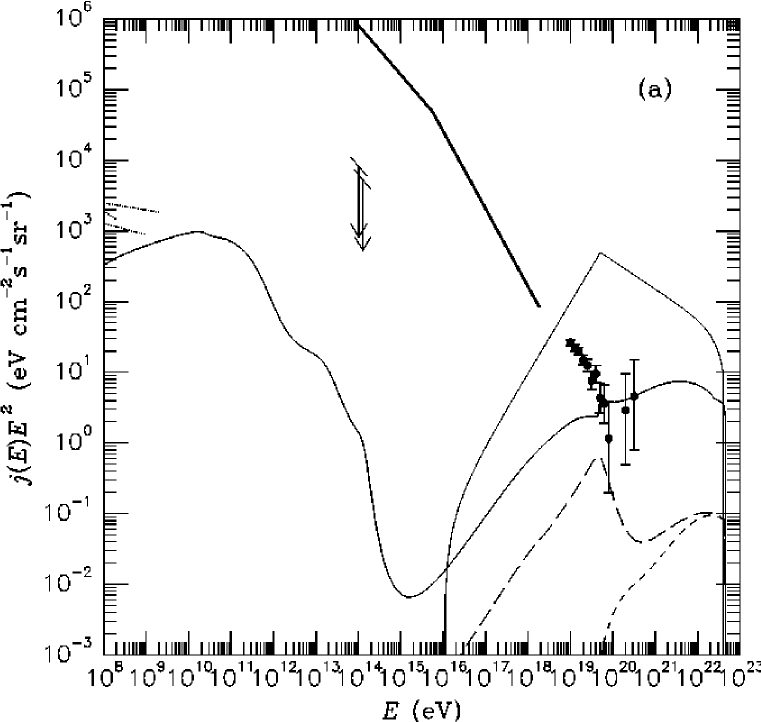
Figure 17: (a) Same as Fig. 14(a), but assuming the fragmentation functions given by Eqs. (51), (52) with $m_{X}=10^{23}{\,{\rm eV}}$.

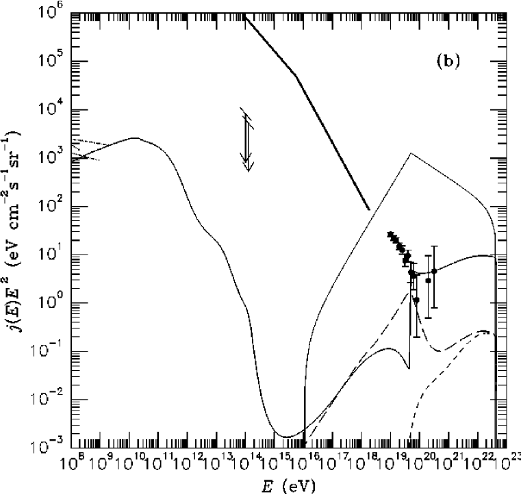
Figure 17: (b) Same as (a), but for an EGMF of $10^{-9}{\,{\rm G}}$.

Fig. 17 shows results obtained by assuming the fragmentation functions given by Eqs. (51), (52). The $100{\,{\rm MeV}}$ $-10{\,{\rm GeV}}$ $\gamma$-ray background constraint is basically unchanged from the case of the QCD motivated injection spectra for vanishing EGMF on which it depends more weakly. Note that this scenario has the potential to explain a HECR spectrum continuing beyond $10^{20}{\,{\rm eV}}$ without any break or gap [13].

5.2 Gamma Ray Burst Models

Recently, it has been suggested that UHE CR could be associated with cosmological GRBs [24, 25, 26]. This was mainly motivated by an apparent numerical coincidence: Assuming that each (cosmological) GRB releases an amount of energy in the form of UHE CRs which is comparable to the total $\gamma$-ray output normalized to the observed GRB rate (about $10^{51}{\,{\rm erg}}$ per burst), the predicted and the observed UHE CR flux at the Earth are comparable. It should be mentioned, however, that it is not clear whether constraints on cosmological GRB distributions are consistent with HECR observations [97].

In these models protons are accelerated to UHE via first order Fermi acceleration. Since there are no firm predictions for the injection spectrum, I assume the hardest possible spectrum proportional to $E^{-2}$ up to a maximal energy of $10^{23}{\,{\rm eV}}$. Furthermore, assuming a constant comoving injection rate up to some maximal redshift $z_{\rm max}$, we can write

$$\Phi_{p}(E,t)\propto t^{-2}E^{-2}\,\Theta(z_{\rm max}-z)\Theta(10^{23}{\,{\rm eV}}-E)\,.$$ (53)

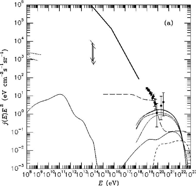
Figure 18: Predictions for the differential fluxes of $\gamma$-rays (solid line), protons (long dashed line), neutrons (short dashed line), and $\nu_{\mu}$, $\bar{\nu}_{\mu}$, $\nu_{e}$, $\bar{\nu}_{e}$ (thin solid lines from the top) by the GRB injection scenario given by Eq. (53) for vanishing EGMF for: (a) $z_{\rm max}=1$. Observational data and constraints are presented as in Fig. 14.

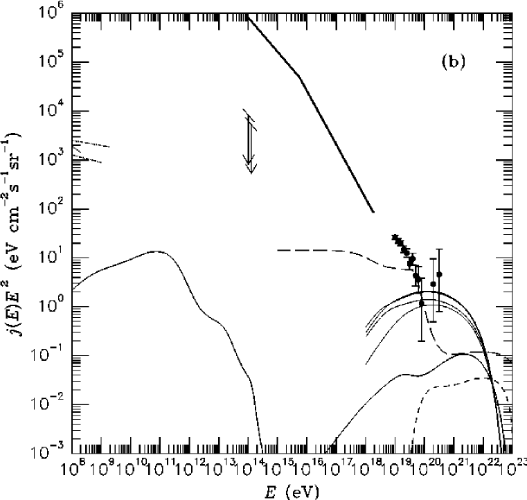
Figure 18: (b) $z_{\rm max}=4$.

The authors of Ref. [26] pointed out that bursting sources in combination with deflection of protons in the EGMF could lead to UHE CR spectra with a time variability on a scale of $\sim 50{\,{\rm yr}}$. This might allow reasonable fits to the observed HECR spectrum. However, I only consider the continuous injection of CRs in this paper for illustrative purposes. Since the $\gamma$-ray background depends only on the average flux, the only uncertainty in its flux level comes from the fit to the HECR events. I estimate the uncertainty introduced by normalizing the average flux to be less than a factor 1.5. Fig. 18 shows the results for various values of $z_{\rm max}$. I conclude that these models are currently unconstrained by the $\gamma$-ray background, although they still have difficulty explaining the highest energy CR events.

6 Conclusions

I have performed detailed numerical simulations for the propagation of extragalactic nucleons, $\gamma$-rays, and electrons in the energy range between $10^{8}{\,{\rm eV}}$ and $10^{23}{\,{\rm eV}}$. My goal was to explore constraints on various models of HECR origin from a comparison of predicted and observed $\gamma$-ray fluxes at lower energies. The main focus thereby is on models which associate HECRs with GUT scale physics or with cosmological GRBs.

I find that at present the TD scenarios are primarily constrained by the observed $\gamma$-ray background between $\simeq 100{\,{\rm MeV}}$ and $\simeq 10{\,{\rm GeV}}$ but not by the limit on the $\gamma$ to charged CR flux ratio below $100\,{\rm TeV}$. The CEL approximation usually does not take the IR/O background into account, and thus may not be directly compared to the numerical calculation because the presence of the IR/O background may affect the $\gamma$-ray flux level at $100\,{\rm MeV}$ by an order of magnitude. There is also a significant difference for the UHE spectrum between predictions by the CEL approximation and my numerical simulation. For an EGMF strength $\mathrel{\mathchoice{\lower 3.6pt\vbox{\halign{$\mathsurround=0pt\displaystyle\hfil#\hfil$\cr<\crcr\sim\crcr}}}{\lower 3.6pt\vbox{\halign{$\mathsurround=0pt\textstyle\hfil#\hfil$\cr<\crcr\sim\crcr}}}{\lower 3.6pt\vbox{\halign{$\mathsurround=0pt\scriptstyle\hfil#\hfil$\cr<\crcr\sim\crcr}}}{\lower 3.6pt\vbox{\halign{$\mathsurround=0pt\scriptscriptstyle\hfil#\hfil$\cr<\crcr\sim\crcr}}}}10^{-11}\,{\rm G}$ the TD models yield the $\gamma$-ray flux which is at about the same level as or below the current observed flux, depending on the adopted parameters. On the other hand, an EGMF stronger than $\sim 10^{-11}\,{\rm G}$ stops the cascade at UHEs and the UHE end of the spectrum is suppressed significantly. Thus, the level of the $\gamma$-ray flux at about $100\,{\rm MeV}$ is higher relatively, tightening the constraints. However, these results are rather insensitive to different models of the IR/O background [63], although they are somewhat dependent on the poorly known universal radio background flux.

I conclude that TD scenarios with QCD motivated injection spectra up to energies $\mathrel{\mathchoice{\lower 3.6pt\vbox{\halign{$\mathsurround=0pt\displaystyle\hfil#\hfil$\cr<\crcr\sim\crcr}}}{\lower 3.6pt\vbox{\halign{$\mathsurround=0pt\textstyle\hfil#\hfil$\cr<\crcr\sim\crcr}}}{\lower 3.6pt\vbox{\halign{$\mathsurround=0pt\scriptstyle\hfil#\hfil$\cr<\crcr\sim\crcr}}}{\lower 3.6pt\vbox{\halign{$\mathsurround=0pt\scriptscriptstyle\hfil#\hfil$\cr<\crcr\sim\crcr}}}}10^{23}{\,{\rm eV}}$ are still viable if injection occurs uniformly or from a discrete source. This is in contrast to a recent claim in the literature [51]. In case of uniform injection this assumes an injection history motivated by energy release from a network of cosmic strings in the scaling regime or from monopole-antimonopole annihilation ($p=1$). Higher injection energy cutoffs are allowed for either a weaker source evolution or for injection spectra somewhat steeper than the QCD motivated spectra. For EGMF strengths larger than $\simeq 10^{-10}{\,{\rm G}}$, some of the predicted TD spectra have the potential to explain a possible gap in the HECR spectrum. The cosmological GRB scenarios recently suggested in the literature [24, 25, 26] are currently unconstrained by these limits.

With the arrival of the anticipated Pierre Auger Cosmic Ray Observatories [57], it is expected that the UHE end of the CR spectrum will be known with much better accuracy. Constraints derived from the influence of CR propagation on the observed spectrum will then be one of the most powerful tools in discriminating between models of HECR origin.

Appendix A: Triplet pair production

The expressions for the differential spectra of produced pairs and the recoiling electron (positron) for TPP by a very energetic electron on a soft photon can be found in many papers [75, 76, 77]. I adopt the analytic approach used in [76]. For an interaction of an electron of energy $E$ with a photon of energy $\epsilon$ ($E\gg\epsilon$), the double differential cross section with respect to the positron produced with energy $E_{+}$ at solid angle $\Omega_{+}$ can be expressed as

$$\frac{d^{2}\sigma}{dE_{+}d\Omega_{p_{+}}}=\sigma_{T}\cdot\frac{3\alpha}{16\pi^{3}}\frac{p_{+}}{p\cdot k}\frac{(\rho_{t}^{2}-4)^{1/2}}{\rho_{t}}\int A_{t}d\Omega_{p^{\prime}},$$ (54)

where $p\cdot k$ is the scalar product of the initial electron and photon four-momenta, $p_{+}$ is the magnitude of the produced positron three-momentum, $\Omega_{p^{\prime}}$ is the solid angle of the recoiling electron, and $\rho_{t}$ and $A_{t}$ are given in Ref. [76]. The single differential cross section with respect to the positron energy may be obtained by integrating Eq. (54) over the positron solid angle $\Omega_{+}$ numerically. The differential cross section for the produced electron is identical to that for the positron due to symmetry. In doing the integral, it is useful to use the approximation where the dependence of the cross section on the azimuthal angle of the outgoing particles in the cosmic ray frame is neglected, as was mentioned before.

Finally, we can obtain the total TPP cross section by integrating Eq. (54) numerically over the kinematic range of electron and positron energies given by

$$E_{\rm max,min}=\frac{E_{\rm tot}(s_{0}-m_{e}^{2})\pm P_{\rm tot}[s_{0}(s_{0}-4m_{e}^{2})]^{1/2}}{2s_{0}+m_{e}^{2}},$$ (55)

where $s_{0}\equiv\epsilon(E+p)$, and $E_{\rm tot}$ and $P_{\rm tot}$ are the total incident energy and momentum, respectively.

I also give here the kinematic energy range for the outgoing electron and positron and the recoiling proton in case of pair production by protons (Section 3.2.1):

$$E_{\rm max,min}=\frac{E_{\rm tot}(s_{0}-m_{e}\lambda)\pm P_{\rm tot}[s_{0}^{2}-2m_{e}s_{0}(m_{e}+\lambda)+m_{e}^{2}(m_{e}^{2}-m_{N}^{2})/2]^{1/2}}{2s_{0}+m_{N}^{2}},$$ (56)

where $s_{0}$ is as defined previously, $\lambda\equiv[(m_{e}^{2}+m_{N}^{2})/2]^{1/2}$.

Appendix B: Photopion production

First, I express the differential cross sections for single pion production in terms of the CRF energies $E^{\prime}_{a}$, where $a=N,\pi$:

$${d\sigma_{i}\over dE^{\prime}_{N}}\,,\,{d\sigma_{i}\over dE^{\prime}_{\pi}} = {2\pi\over E_{N}}\,{1+2\kappa\over D}\,\sum_{j=0}^{K}a_{ij}(\kappa)\left(x^{*}\right)^{j}$$ (59)

$$\times\left\{\begin{array}[]{ll}1&\mbox{for $i=1$ (charge retention)}\\ \left(1-\beta^{*}x^{*}\right)^{-1/2}&\mbox{for $i=2,3$ (charge exchange)}\end{array}\right.$$

where $\beta^{*}=D/(\kappa+\varepsilon^{2}/2)$ and $x^{*}$ can be expressed as a function of $E^{\prime}_{N}$ or $E^{\prime}_{\pi}$ and $E_{N}$:

$$x^{*}=\frac{(1+2\kappa)(E^{\prime}_{N}/E_{N})-1-\kappa-\varepsilon^{2}/2}{D}=-\frac{(1+2\kappa)(E^{\prime}_{\pi}/E_{N})-\kappa-\varepsilon^{2}/2}{D}\,.$$ (60)

Finally, I compute the fractions $r_{c}(\kappa)$ and $r_{\rho}(\kappa)$ of the incoming nucleon energy going into the central and leading pions. These fractions are given by integrating the differential cross section $d\sigma/dE_{\pi}$ for the respective process, weighted by the pion energy $E_{\pi}$, in the CRF, and dividing by the corresponding total cross section. Using Eq. (35),

$$E_{\pi}={E_{N}\over m_{N}}\,{E_{\pi}^{*}-p_{\|}^{*}\over(1+2\kappa)^{1/2}}={E_{N}\over m_{N}}{p_{\rm max}^{*}\over(1+2\kappa)^{1/2}}\left[\left(x^{2}+{p_{\bot}^{2}+m_{\pi}^{2}\over(p_{\rm max}^{*})^{2}}\right)^{1/2}-x\right]\,,$$ (61)

and Eq. (34), we end up with

$$r_{\rho}(\kappa) = {\pi\over\sigma_{\rho}}\,{D\over 1+2\kappa}$$

$$\times\int dp_{\bot}^{2}\int dx\,2f_{\rho}(x)\frac{\exp[-p_{\bot}^{2}/\Lambda^{2}]}{\Lambda^{2}}\left\{1-x\left[x^{2}+\frac{1+2\kappa}{D^{2}}\left({p_{\bot}^{2}\over m_{N}^{2}}+\varepsilon^{2}\right)\right]^{-1/2}\right\}\,.$$

Again, the integration ranges are obtained by the requirement $p_{\bot}^{2}/(p_{\rm max}^{*})^{2}+x^{2}\leq 1$. The formula for $r_{c}(\kappa)$ can be obtained from this by substituting $\sigma_{\rho}\rightarrow\sigma_{\rm tot}-\sigma_{\rho}$ and $2f_{\rho}(x)\rightarrow\left[3+(2/5)(1-\sigma_{\rho}/\sigma_{\rm tot})/\left\langle n_{\pi^{-}}^{c}\right\rangle(\kappa)\right]f_{c}(x)$, where $\left\langle n_{\pi^{-}}^{c}\right\rangle(\kappa)$ was given in Eq. (40).

Appendix C: Pion decay spectra

First, we define the decay spectrum $N_{a}(E)$ as the differential number of the secondary particle $a$ at energy $E$. Then the spectrum is normalized as

$$\int dEN_{a}(E)=n_{a},$$ (63)

where $n_{a}$ is the number of particles $a$ produced by decay of a single pion. For example, $n_{\gamma}=2$ for $\pi^{0}$ decay.

First, the photon spectrum from $\pi^{0}$ decay is

$$N_{\gamma}(E)=\frac{2}{E_{\pi}}\quad\mbox{for $E\leq E_{\pi}$}\,.$$ (64)

Before we calculate the charged pion decay spectra, we note the fact that the pions produced from photopion production are always relativistic. Thus, we may make the relativistic approximation for both pions and the resulting muons. For example, the decay spectra of $\pi^{+}$ read:

$$N_{e^{+}}(E) = N_{\bar{\nu}_{\mu}}(E)\simeq\left\{\begin{array}[]{ll}\frac{1}{(1-r)E_{\pi}}(A_{0}+A_{2}z^{2}+A_{3}z^{3})&\mbox{for $E\leq rE_{\pi}$}\\ \frac{1}{(1-r)E_{\pi}}(B_{0}+B_{0}^{\prime}\ln z+B_{2}z^{2}+B_{3}z^{3})&\mbox{for $rE_{\pi}\mathrel{\mathchoice{\lower 3.6pt\vbox{\halign{$\mathsurround=0pt\displaystyle\hfil#\hfil$\cr<\crcr\sim\crcr}}}{\lower 3.6pt\vbox{\halign{$\mathsurround=0pt\textstyle\hfil#\hfil$\cr<\crcr\sim\crcr}}}{\lower 3.6pt\vbox{\halign{$\mathsurround=0pt\scriptstyle\hfil#\hfil$\cr<\crcr\sim\crcr}}}{\lower 3.6pt\vbox{\halign{$\mathsurround=0pt\scriptscriptstyle\hfil#\hfil$\cr<\crcr\sim\crcr}}}}E\leq E_{\pi}$},\end{array}\right.$$ (75)

$$N_{\nu_{\mu}}(E) = {1\over(1-r)E_{\pi}}\quad\mbox{for $E\leq(1-r)E_{\pi}$}$$ (76)

$$N_{\nu_{e}}(E) \simeq \left\{\begin{array}[]{ll}\frac{1}{(1-r)E_{\pi}}(C_{0}+C_{2}z^{2}+C_{3}z^{3})&\mbox{for $E\leq rE_{\pi}$}\\ \frac{1}{(1-r)E_{\pi}}(D_{0}+D_{0}^{\prime}\ln z+D_{1}z+D_{2}z^{2}+D_{3}z^{3})&\mbox{for $rE_{\pi}\leq E\leq E_{\pi}$},\end{array}\right.\,,$$ (79)

where $r\equiv m_{\mu}^{2}/m_{\pi}^{2}$, $z\equiv E/E_{\pi}$, and coefficients are given as

$$(A_{0},A_{2},A_{3})=(0.94486,-2.7892,1.2397),$$

$$(B_{0},B_{0}^{\prime},B_{2},B_{3})=(-2.4126,-2.8951,4.3426,-1.9300),$$

$$(C_{0},C_{2},C_{3})=(1.1053,-4.46883,3.71887),$$

and

$$(D_{0},D_{0}^{\prime},D_{1},D_{2},D_{3})=(13.846,5.37053,-28.1116,20.0558,-5.7902).$$

The average energies of the secondary particles are $\langle E_{e^{+}}\rangle=\langle E_{\bar{\nu}_{\mu}}\rangle=0.265E_{\pi}$, $\langle E_{\nu_{e}}\rangle=0.257E_{\pi}$, and $\langle E_{\nu_{\mu}}\rangle=0.213E_{\pi}$ respectively. The decay spectra from $\pi^{-}$ are obtained by substituting particles accordingly.

Figure 1: The universal background radiation intensity spectrum at $z=0$ (solid line) used in our model. The separate contributions from the radio (short dashed line), the IR/O (long dashed line) background, and the CMB (dotted line) are also shown.

Figure 2: The effective comoving density of radio and IR/O sources whose luminosities are normalized at $z=0$, as a function of redshift. This corresponds to $N_{c}(z)$ in Eq. (3). The IR/O source density is assumed to cut off at $z=5$.

Figure 3: Gyroradii (dashed lines) and synchrotron loss lengths (solid lines) of electrons for various strengths of the EGMF in units of gauss (G) as indicated.

Figure 4: The total cross sections, $\sigma(s)$, and the cross sections times the average inelasiticity, $\sigma(s)\eta(s)$, which is proportional to the fractional energy loss rate of the leading particle: (a) For PP (solid line and short dashed line, respectively) and DPP (dotted line).

Figure 4: (b) For ICS (solid line and short dashed line, respectively) and TPP (dotted line and long dashed line, respectively).

Figure 6: (a) The fractions $r_{c}$ and $r_{\rho}$ of the incoming nucleon energy which goes into the central and leading pions, respectively, as functions of $s$.

Figure 6: (b) The average central and total $\pi^{-}$ multiplicities, $\left\langle n_{\pi^{-}}^{c}\right\rangle$ [see Eq. (40)] and $\left\langle n_{\pi^{-}}\right\rangle$ [resulting by substituting $f_{c}(x)\rightarrow f(x)$ in Eq. (40)] as functions of $s$.

Figure 7: The differential cross sections for production of $\pi^{-}$ (dotted lines), $\pi^{+}$ (short dashed lines), $\pi^{0}$ (solid lines), protons (long dashed lines), and neutrons (dash-dotted lines) for the collision of a proton of energy $E$ with a background photon at squared CM energy $s$, from the formalism adopted in Section 3.2.2: (a) For $E=3\times 10^{20}{\,{\rm eV}}$, $s=2.1{\,{\rm GeV}}^{2}$.

Figure 7: (b) For $E=3\times 10^{22}{\,{\rm eV}}$, $s=120{\,{\rm GeV}}^{2}$.

Figure 8: The inclusive multiple pion production cross section for protons (solid line) and neutrons (dashed line) as a function of $s$.

Figure 9: The interaction rates and energy attenuation rates for multiple pion production (solid line and short dashed line, respectively) and PPP (dotted line and long dashed line, respectively). The rates were obtained by folding the cross sections and inelasticity weighted cross sections with the present background photon spectrum shown in Fig 2.

Figure 10: The energy attenuation lengths for cascade photons and for protons as a function of energy assuming the radiation background photon spectrum shown in Fig. 2. These curves were obtained by running the code over small distances and ignoring the production of non-leading particles, which corresponds to the CEL approximation.

Figure 11: The modification factors as defined in Ref. [44] for discrete sources injecting a $E^{-2}$ proton spectrum extending up to $3\times 10^{20}{\,{\rm eV}}$ at a given distance $d$ or redshift $z$ resulting from our analysis (solid lines). Also shown are the corresponding curves from Protheroe and Johnson [51] (dashed lines): (a) For $d=256{\,{\rm Mpc}}$. For further comparison with results from Refs. [44, 47] see the discussion in Ref. [51].

Figure 11: (b) For $z=0.6$.

Figure 11: (c) For $z=1$.

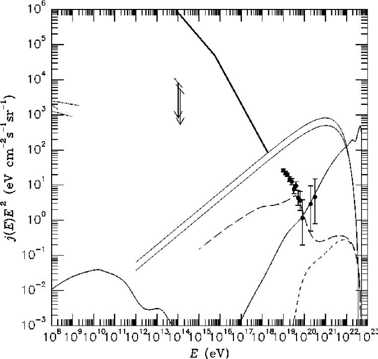
Figure 15: Same as Fig. 14(a), but neglecting non-leading particles in the EM cascade development. Only the UHE part is important in comparison with Fig. 14(a).

Figure 16: (b) Same as Fig. 14(a), but for an EGMF of $10^{-11}\,$G.

References

- [1] A. A. Penzias and R. W. Wilson, Astrophys. J. 142, 419 (1965).
- [2] K. Greisen, Phys. Rev. Lett. 16, 748 (1966); G. T. Zatsepin and V. A. Kuz’min, Pis’ma Zh. Eksp. Teor. Fiz. 4, 114 (1966) [JETP. Lett. 4, 78 (1966)].
- [3] F. W. Stecker, Phys. Rev. Lett. 21, 1016 (1968).
- [4] J. L. Puget, F. W. Stecker, and J. H. Bredekamp, Astrophys. J. 205, 638 (1976).
- [5] Astrophysical Aspects of the Most Energetic Cosmic Rays, edited by M. Nagano and F. Takahara (World Scientific, Singapore, 1991).
- [6] Proceedings of the Tokyo Workshop on Techniques for the Study of Extremely High Energy Cosmic Rays, Tokyo, Japan, 1993 (Institute for Cosmic Ray Research, Univ. of Tokyo, 1993).
- [7] M. A. Lawrence, R. J. O. Reid, and A. A. Watson, J. Phys. G Nucl. Part. Phys. 17, 733 (1991); A. A. Watson in Ref. [5], p.2.
- [8] D. J. Bird et al., Phys. Rev. Lett. 71, 3401 (1993); Astrophys. J. 424, 491 (1994).
- [9] D. J. Bird et al., Astrophys. J. 441, 144 (1995).
- [10] N. N. Efimov et al. in Ref. [5], p. 20; T. A. Egorov in Ref. [6], p. 35.
- [11] S. Yoshida et al., Astropart. Phys. 3, 105 (1995).
- [12] N. Hayashida et al., Phys. Rev. Lett. 73, 3491 (1994).
- [13] G. Sigl, S. Lee, D. N. Schramm, and P. Bhattacharjee, Science 270, 1977 (1995).
- [14] A. M. Hillas, Ann. Rev. Astron. Astrophys. 22, 425 (1984).
- [15] W. H. Sorrell in Ref. [5], p. 329.
- [16] P. Sommers in Ref. [6], p. 23.
- [17] J. W. Elbert and P. Sommers, Astrophys. J. 441, 151 (1995).
- [18] G. Sigl, D. N. Schramm, and P. Bhattacharjee, Astropart. Phys. 2, 401 (1994).
- [19] For a review see R. Blandford and D. Eichler, Phys. Rep. 154, 1 (1987).
- [20] T. K. Gaisser, Cosmic Rays and Particle Physics (Cambridge University Press, Cambridge, 1990).
- [21] P. L. Biermann and P. A. Strittmatter, Astrophys. J. 322, 643 (1987).
- [22] C. T. Cesarsky, Nucl. Phys. B (Proc. Suppl.) 28B, 51 (1992).
- [23] C. A. Norman, D. B. Melrose, and A. Achterberg, Astrophys. J. 454, 60 (1995).
- [24] E. Waxman, Astrophys. J. 452, L1 (1995).
- [25] M. Vietri, Astrophys. J. 453, 883 (1995).
- [26] J. Miralda-Escude and E. Waxman, preprint astro-ph/9601012 (unpublished).
- [27] C. T. Hill, Nucl. Phys. B 224, 469 (1983).
- [28] C. T. Hill, D. N. Schramm, and T. P. Walker, Phys. Rev. D 36, 1007 (1987).
- [29] P. Bhattacharjee, Phys. Rev. D 40, 3968 (1989).
- [30] P. Bhattacharjee in Ref. [5], p. 382.
- [31] P. Bhattacharjee and N. C. Rana, Phys. Lett. B 246, 365 (1990).
- [32] P. Bhattacharjee, C. T. Hill, and D. N. Schramm, Phys. Rev. Lett. 69, 567 (1992).
- [33] P. Bhattacharjee and G. Sigl, Phys. Rev. D 51, 4079 (1995).
- [34] G. Sigl, Space Science Reviews (to be published).
- [35] Proceedings of 24th International Cosmic Ray Conference, Rome, Italy, 1995 (Istituto Nazionale Fisica Nucleare, Rome, 1995).
- [36] T. Doi et al., in Ref. [35], Vol. 2, p. 740.
- [37] F. Halzen, R. A. Vazquez, T. Stanev, and H. P. Vankov, Astropart. Phys. 3, 151 (1995).
- [38] T. K. Gaisser (private communication).
- [39] T. Weiler, Phys. Rev. Lett. 49, 234 (1982); Astrophys. J. 285, 495 (1984).
- [40] S. Yoshida, Astropart. Phys. 2, 187 (1994).
- [41] G. Sigl and S. Lee, in Ref. [35], Vol. 3, p. 356.
- [42] V. S. Berezinsky and S. I. Grigor’eva, Astron. Astrophys. 199, 1 (1988).
- [43] F. A. Aharonian, B. L. Kanevsky, and V. V. Vardanian, Astrophys. Space Sci. 167, 93 (1990).
- [44] J. P. Rachen, and P. L. Biermann, Astron. Astrophys. 272, 161 (1993).
- [45] J. Geddes, T. C. Quinn, and R. M. Wald, Astrophys. J. 459, 384 (1996).
- [46] C. T. Hill and D. N. Schramm, Phys. Rev. D 31, 564 (1985).
- [47] S. Yoshida and M. Teshima, Prog. Theor. Phys. 89, 833 (1993).
- [48] F. A. Aharonian and J. W. Cronin, Phys. Rev. D 50, 1892 (1994).
- [49] J. Wdowczyk and A. W. Wolfendale, Astrophys. J. 349, 35 (1990).
- [50] F. A. Aharonian, P. Bhattacharjee, and D. N. Schramm, Phys. Rev. D 46, 4188 (1992).
- [51] R. J. Protheroe and P. A. Johnson, Astropart. Phys. (to be published).
- [52] S. Lee, A. V. Olinto, and G. Sigl, Astrophys. J. 455, L21 (1995).
- [53] S. Lee and G. Sigl, in Ref. [35], Vol. 2, p. 536.
- [54] F. W. Stecker and O. C. De Jager, Astrophys. J. 415, L71 (1993); O. C. De Jager, F. W. Stecker, and M. H. Salamon, Nature 369, 294 (1994).
- [55] F. Halzen, R. J. Protheroe, T. Stanev, and H. P. Vankov, Phys. Rev. D 41, 342 (1990).
- [56] G. Sigl, K. Jedamzik, D. N. Schramm, and V. Berezinsky, Phys. Rev. D 52, 6682 (1995).
- [57] See, for example, Proceedings of the International Workshop on Techniques to Study Cosmic Rays with Energies , Paris, France, 1992, edited by M. A. Boratav, J. W. Cronin, and A. A. Watson [Nucl. Phys. B (Proc. Suppl.) 28B (1992)].
- [58] S. W. Digel, S. D. Hunter, and R. Mukherjee, Astrophys. J. 441, 270 (1995).
- [59] C. E. Fichtel et al., Astrophys. J. 217, L9 (1977); D. J. Thompson and C. E. Fichtel, Astron. Astrophys. 109, 352 (1982).
- [60] J. L. Osborne, A. W. Wolfendale, and L. Zhang, J. Phys. G 20, 1089 (1994).
- [61] For a standard textbook discussion, see J. D. Jackson, Classical Electrodynamics, 2nd Ed. (John Wiley & Sons, New York, 1975).
- [62] M. T. Ressell and M. S. Turner, Comments Astrophys. 14, 323 (1990).
- [63] P. S. Coppi and F. A. Aharonian (unpublished).
- [64] F. W. Stecker, O. C. De Jager, and M. H. Salamon, Astrophys. J. 390, L49 (1992).
- [65] D. MacMinn and J. R. Primack, Space Science Reviews (to be published).
- [66] P. Mazzei, C. Xu, and G. De Zotti, Astron. Astrophys. 256, 45 (1992).
- [67] T. A. Clark, L. W. Brown, and J. K. Alexander, Nature 228, 847 (1970).
- [68] M. S. Longair and R. Sunyaev, Usp. Fiz. Nauk 105, 41 (1971) [Sov. Fiz. Usp. 14, 569 (1971)].
- [69] J. S. Dunlop and J. A. Peacock, Mon. Not. R. Astron. Soc. 247, 19 (1990).
- [70] P. S. Coppi and A. Königl (unpublished).
- [71] R. J. Protheroe and T. S. Stanev, Mon. Not. R. Astron. Soc. 264, 191 (1993).
- [72] A. A. Zdziarski, Astrophys. J. 335, 786 (1988).
- [73] P. S. Coppi and R. D. Blandford, Mon. Not. R. Astron. Soc. 245, 453 (1990).
- [74] R. W. Brown et al., Phys. Rev. D 8, 3083 (1973).
- [75] A. Mastichiadis, Mon. Not. R. Astron. Soc. 253, 235 (1991).
- [76] E. Haug, Zeit. Naturforsch. 30a, 1099 (1975).
- [77] A. Borsellino, Nuovo Cimento 4, 112 (1947).
- [78] W. Rhode et al., Astropart. Phys. (to be published).
- [79] K.-T. Kim et al., Nature 341, 720 (1989); P. P. Kronberg, Rep. Prog. Phys. 57, 325 (1994).
- [80] R. J. Gould, Astrophys. J. 230, 967 (1979).
- [81] R. Svensson and A. A. Zdziarski, Astrophys. J. 349, 415 (1990).
- [82] A. A. Zdziarski and R. Svensson, Astrophys. J. 344, 551 (1989).
- [83] G. R. Blumenthal, Phys. Rev. D 1, 1596 (1970).
- [84] J. W. Motz, H. A. Olsen, and H. W. Koch, Rev. Mod. Phys. 41, 581 (1969).
- [85] M. J. Chodorowski, A. A. Zdziarski, and M. Sikora, Astrophys. J. 400, 181 (1992).
- [86] H. Genzel, P. Joos, and W. Pfeil, in Landolt and Börnstein: Photoproduction of Elementary Particles (1973), Vol. 8, p. 1.
- [87] K. C. Moffeit et al., Phys. Rev. D 5, 1603 (1972).
- [88] R. P. Feynman, Phys. Rev. Lett. 23, 1415 (1969).
- [89] C. T. Hill and D. N. Schramm, Phys. Lett. B 131, 247 (1983).
- [90] F. Halzen and A. D. Martin, Quarks & Leptons: an Introductory Course in Modern Particle Physics (John Wiley & Sons, New York, 1984).
- [91] see, e.g., E. W. Kolb and M. S. Turner, The Early Universe (Addison-Wesley, New York, 1990).
- [92] A. Vilenkin, Phys. Rep. 121, 263 (1985).
- [93] A. Karle et al., Phys. Lett. B 347, 161 (1995).
- [94] X. Chi, C. Dahanayake, J. Wdowczyk, and A. W. Wolfendale, Astropart. Phys. 1, 129 (1993).
- [95] X. Chi, C. Dahanayake, J. Wdowczyk, and A. W. Wolfendale, Astropart. Phys. 1, 239 (1993).
- [96] G. Sigl, S. Lee, and P. S. Coppi (unpublished).
- [97] J. M. Quashnock, Astrophys. J. Lett (to be published).