Abstract

This review is a short introduction to numerical hydrodynamics in a cosmological context, intended for the non specialist. The main processes relevant to galaxy formation are first presented. The fluid equations are then introduced, and their implementation in numerical codes by Eulerian grid based methods and by Smooth Particle Hydrodynamics is sketched. As an application, I finally show some results from an SPH simulation of a galaxy cluster.

HYDRODYNAMIC SIMULATIONS
OF GALAXY FORMATION

Institute of Astronomy, University of Cambridge - ENGLAND and Max-Planck-Institut für Astrophysik, Garching - GERMANY

1 Gas Physical Processes

In current cosmological scenarios, the main matter components of the universe are some non baryonic Dark Matter (DM), which constitutes most of the universe, and a mixture of primordial gas (H, He). The DM component is decoupled from the rest of the universe, and interacts only through gravity. The gas component instead can be heated and cooled in several ways, and the physics involved is more complicated than in the pure gravitational case. Fortunately, while gravity is a long range force, hydrodynamic processes are only important on relatively small scales, so that on scales larger than a few Mpc the dynamics of structure formation can be studied with good accuracy even neglecting the gas component. Gas dynamics, and the related radiative processes, are instead fundamental on smaller scales, e.g. in the formation of galaxies, and in linking the matter distribution of the universe to the light distribution we actually observe¹⁾. In what follows I list and discuss very briefly the main gas processes relevant to galaxy formation.

1.1 Heating processes

Adiabatic compression

is the easiest way to heat a gas. By the First Law of Thermodynamics, compression work is converted into internal energy: $dQ=dU+pdV=0\Longrightarrow dU=-pdV$.

Viscous heating

is due to the small internal friction (viscosity) present in real gas. Velocity gradients in a gas cause an irreversible transfer of momentum from high velocity points to small velocity ones, with conversion of bulk velocities into random ones, i.e. into heat, and generation of entropy. In the context of galaxy formation viscous heating mostly occurs in shocks, which are discontinuities in the macroscopic fluid variables due to supersonic flows. These arise for example during gravitational collapse, or during supernova (SN) explosions.

Photoionization

takes place when atoms interact with the photons of some background of soft X-rays, or UV radiation emitted by QSO or stars: e.g. $\gamma+H\rightarrow e^{-}+H^{+}$. Observations show that at high redshift ($z~{}\hbox to0.0pt{$>$\hss}{\lower 4.30554pt\hbox{$\sim$}}2$) hydrogen in the IGM is indeed ionized (Gunn-Peterson effect²⁾), and although the origin is not clear, this is thought to be caused by some early generation of QSO or massive stars. The photoionizing spectrum is usually approximated by a power law, with flux $J(\nu)\propto(\nu/\nu_{L})^{-\alpha}$, where $\nu_{L}$ is the Lyman-$\alpha$ frequency, corresponding to the hydrogen ionization energy, $13.6$ eV.

1.2 Cooling processes

Gas cooling is the key to galaxy formation. In fact, in our current understanding of structure formation, the dark matter component of the universe first undergoes gravitational collapse, forming dark matter halos. These provide the potential wells into which gas can fall and heat up by shocks, then immediately cool and form cold, dense, rotationally supported gas disks. In these disks conditions are favourable to trigger star formation, and eventually give rise to the galaxies we observe today³⁾. The following cooling mechanisms are important in a cosmological context.

Adiabatic expansion

is the opposite process of adiabatic compression, with conversion of heat into expansion work.

Compton cooling

is electron cooling against the Cosmic Microwave Background (CMB) through inverse Compton effect: $\gamma+e^{-}\rightarrow\gamma+e^{-}$. The condition for this is that the temperature of the electrons is higher than the CMB temperature: $T_{e}>T_{\gamma}$. The net energy transfer depends on the two densities, and on the temperature difference: $dE/dT\propto n_{e}\rho_{\gamma}(T_{e}-T_{\gamma})$. Since $E\propto n_{e}T_{e}$, the cooling time: $t_{cool}\equiv E/\dot{E}$ is in this case $\propto\rho_{\gamma}^{-1}$. The CMB photon density decreases like $(1+z)^{4}$ due to the expansion of the universe, therefore Compton cooling is only important at high redshifts (typically $z~{}\hbox to0.0pt{$>$\hss}{\lower 4.30554pt\hbox{$\sim$}}8$), when the cooling timescale is smaller than the Hubble time.

Radiative cooling

is the most relevant mechanism for the cooling of primordial gas. It is caused by inelastic collisions between free electrons and H, He atoms (or their ions). Assuming that the gas is optically thin and in ionization equilibrium, the cooling rate per unit volume may be written $dE/dt\equiv\Lambda(\rho,T)=n_{e}n_{i}f(T)$, where $n_{e}$ and $n_{i}$ are the number densities of free electrons and of atoms (or ions), and $f(T)$ is called cooling function. The main processes are:

• Collisional ionization: the inelastic scattering of a free electron and an atom (or ion), which unbinds one electron from the latter, e.g. $e^{-}+H\rightarrow H^{+}+2e^{-}$. The net cooling for the system is equal to the extraction energy.

• Collisional excitation + line cooling: the same situation as above, but the atom is only excited, and it then decays to the ground state, emitting a photon, e.g. $e^{-}+H\rightarrow e^{-}+H^{*}\rightarrow e^{-}+H+\gamma$. This is the dominant cooling process at low ($10^{4}$ K$~{}\hbox to0.0pt{$<$\hss}{\lower 4.30554pt\hbox{$\sim$}}T~{}\hbox to0.0pt{$<$\hss}{\lower 4.30554pt\hbox{$\sim$}}10^{6}~{}$K) temperatures.

• Recombination: e.g. $e^{-}+H^{+}\rightarrow H+\gamma$. A free electron is captured by an ion and emits a (continuum) photon.

• Bremsstrahlung: free-free scattering between a free electron and an ion, e.g. $e^{-}+H^{+}\rightarrow e^{-}+H^{+}+\gamma$. Its cooling rate grows with the temperature: $dE/dt\propto T^{1/2}$; therefore, bremsstrahlung is the dominant cooling process at high ($T~{}\hbox to0.0pt{$>$\hss}{\lower 4.30554pt\hbox{$\sim$}}10^{6}$ K) temperatures.

Figure 1 shows the cooling and heating functions in different cases.

Figure 1: Cooling and heating functions. Left panel: cooling function $\Lambda(T)/n_{H}^{2}$ versus temperature, for a primordial gas. The different contributions to radiative cooling, and the total cooling curve are indicated. No photoionizing background is assumed. Right panel: a heating term $\Gamma/n_{H}^{2}$ is added, due to a photoionizing UV background with spectral index $\alpha=1.5$. Its effect is both to change the ionization equilibrium (and so to change $\Lambda(T)/n_{H}^{2}$), and to heat the gas. Thin lines correspond to a gas density equal to the mean background density at redshift $z=5$; thick lines correspond to a density 200 times larger. For low density gas the effect of a UV background is dramatic, and line cooling is suppressed. The temperature $T_{eq}$ where $|\Lambda-\Gamma|$ drops to zero is called equilibrium temperature. At $T>T_{eq}$ the gas is cooled, at $T<T_{eq}$ it is heated. This figure was kindly prepared by I.Forcada using the atomic rates provided by T.Abel.

1.3 Other processes

Besides the heating and cooling mechanisms listed above, other processes may be relevant in a galaxy formation scenario. Among them:

Thermal conduction

is direct transfer of heat from regions at high temperature to regions at lower temperature, due to the energy transport of diffusing electrons. The induced change in internal energy per unit volume is $dE/dT=\vec{\nabla}\left(\kappa\vec{\nabla}T\right)$, with (positive) thermal conductivity $\kappa=\kappa(T,p)$.

Radiation transfer

is important in an optically thick medium. Photons are absorbed by gas clouds, thermalized by multiple scattering and reemitted as Black Body radiation. This process depends on the optical depth $\tau_{opt}$ of the gas.

Star formation

follows gas cooling as the next natural step in modeling galaxy formation. Our understanding of the detailed physics of star formation is still rather poor, so what is usually done is to use some empirical prescription to characterize the gas which is supposed to turn into stars. A good example of recipe⁴⁾ is to require: i) a convergent gas flow: $\vec{\nabla}\cdot\vec{v}<0$; ii) a Jeans’ instability criterion: the free-fall time of the gas cloud be less than its sound crossing time; iii) a minimum number density of H atoms, e.g. $n_{H}>0.1$ cm^-3; iv) a minimum gas overdensity, e.g. $\rho_{g}~{}\hbox to0.0pt{$>$\hss}{\lower 4.30554pt\hbox{$\sim$}}\rho_{V}=178\bar{\rho_{g}}$, where $\rho_{V}$ is the virial density of the spherical collapse model, and $\bar{\rho_{g}}$ is the mean background gas density. If all these conditions are satisfied, the gas will form stars at a formation rate similar to the one observed in e.g. spiral galaxies.

Assuming some Initial Mass Function for the stars so formed, it is possible to compute the fraction of gas forming massive stars ($M\geq 8M_{\odot}$). These stars will explode as Type II SN, each one releasing $10^{51}$ erg of energy back in the ISM, causing new shocks and gas heating, and triggering further star formation. It is also possible to include in this recipe gas release and metal enrichment from SN explosions. Unfortunately, at this point the physics of star formation is still poorly understood, and the resulting scenarios depend very much on the kind of assumptions and modeling made.

2 Fluid Equations

For our purpose it is useful to treat the gas as a continuum, and to resort to a hydrodynamic description. The fluid equations express conservation of mass (continuity equation), of momentum (Euler equation) and of energy. We also need an adiabatic state equation: $ds/dt=0$ or $p=p(\rho,T)$. These equations may be written as

$${d\rho\over dt}=-\rho\vec{\nabla}\cdot\vec{v},$$ (1)

$$\rho{d\vec{v}\over dt}=-\vec{\nabla}p+\mathrm{viscosity\ terms}-\rho\vec{\nabla}\Phi,$$ (2)

$$\rho{d\epsilon\over dt}=-p\vec{\nabla}\cdot\vec{v}+\mathrm{viscosity\ terms}+\vec{\nabla}\cdot\left(\kappa\vec{\nabla}T\right)+\left(Q-\Lambda\right),$$ (3)

$$p=p(\rho,T).$$ (4)

Equation (3) is given in terms of the specific internal energy $\epsilon$. In Equations (1) to (3) the lhs and the first term on the rhs constitute the usual fluid equations for a perfect adiabatic gas. The extra terms on the rhs are the nonadiabatic terms introduced in the previous Section. Gravity is included in the Euler equation via the gravitational potential $\Phi$. Artificial viscosity terms must be included to enable the numerical treatment of shocks and entropy production, processes that do not exist in a perfect adiabatic gas. The terms $Q$ and $\Lambda$ denote respectively the heat sources: photon absorption (e.g. photoionization) and energy feedback from SN, and the heat sinks: Compton and radiative cooling, and other photon emission processes. Including all these processes (and others, e.g. magnetic fields) in a recipe for galaxy formation is not an easy task. Limits arise both from the computational limitations of present day machines, and from our ignorance of the physics involved (e.g. the epoch and spectrum of a photoionizing background, or the mechanism and role of energy feedback from stars and SN). Moreover, some processes naturally go with others, so that if cooling is implemented, star formation and energy feedback should also be modeled. For these reasons, different physical processes may or may not be taken into account in different computations. For example, current hydrodynamic simulations of structure formation sometimes include cooling processes, less often photoionization and star formation. On the other hand, thermal conduction and radiative transport have been so far neglected. The former may play a role in the central part of a system, but its efficiency would depend on the presence of (unknown) magnetic fields. Ignoring the latter is probably a good approximation everywhere except in very dense, optically thick regions. Galaxy cluster formation is a neat application of these methods, because cooling and star formation are less crucial here than in galaxy formation, so they can be ignored to first approximation. An example of hydrodynamic simulation of the formation of a galaxy cluster is briefly presented in the last Section of the paper.

2.1 Eulerian Methods

There are two basic ways to numerically solve the above set of equations: Eulerian and Lagrangian. Eulerian methods solve the fluid equations on a discrete grid fixed in space. In the traditional formulation, a Taylor expansion of the terms is used to build a smooth solution of the differential equations across different grid cells, as follows. Let $f$ be a one dimensional scalar field, and $F$ its flux; the conservation equation for $F$ is

$${\partial f\over\partial t}=-{\partial F\over\partial x};$$ (5)

if we Taylor expand $f(x,t)$ in time:

$$f(x,t+dt)=f(x,t)+{\partial f\over\partial t}dt+{1\over 2}{\partial^{2}f\over\partial t^{2}}dt^{2}+O(dt^{3})$$ (6)

and insert Eq. (5) into Eq. (6), we can substitute all time derivatives with spatial ones:

$$f(x,t+dt)=f(x,t)-{\partial F\over\partial x}dt+{1\over 2}{\partial\over\partial x}\left[{\partial F\over\partial x}{\partial F\over\partial f}\right]dt^{2}+O(dt^{3}).$$ (7)

This is the time evolution equation for $f(x,t)$, which is discretized and solved on a grid, to first or second order accuracy. Macroscopic discontinuities in the flow, like those caused by shocks, are mimicked by smooth solutions, obtained introducing explicitly, in the fluid equations, the artificial viscosity terms mentioned above. The underlying idea is that in a real fluid shocks are smooth solutions if seen at small enough scale.

More recent techniques, named shock capturing schemes or Riemann solvers, use a different approach. They incorporate in the method the exact solution of a simple nonlinear problem, the Riemann shock tube. This solution describes the nonlinear waves generated by a discontinuous jump separating two constant states. The fluid flow is then approximated by a large number of constant states for which the Riemann shock tube problem is solved. This automatically leads to an accurate approximation of both smooth solutions and of shocks, with no need of explicitly introducing viscosity terms in the equations. This category of techniques includes the Piecewise Parabolic Method⁵⁾ (PPM) and the Total Variation Diminishing⁶⁾ scheme (TVD).

2.2 Lagrangian methods: SPH

Smooth Particle Hydrodynamics^7),8) (SPH) is the most commonly used Lagrangian method in dissipative simulations of galaxy formation. By analogy with $N$-body codes, where a collisionless fluid is represented with a set of discrete particles, SPH also uses particles to describe the evolution of a gas fluid. Each particle $i$ is assigned a position $\vec{r}_{i}$, a velocity $\vec{v}_{i}$, a density $\rho_{i}$ and a specific internal energy $\epsilon_{i}$, and the fluid equations are solved at the particle’s position, replacing the true fields with smoothed estimates, which are obtained as local averages of the particles’ properties. For example, for a scalar field $f$, the smoothed counterpart $\langle f\rangle$ is:

$$\langle f(\vec{r})\rangle=\int d^{3}uf(\vec{u})W(\vec{r}-\vec{u};h);$$ (8)

$W(\vec{r}-\vec{u};h)$ is the smoothing kernel, strongly peaked at zero, so that

$${\mathrm{lim}}_{h\to 0}\langle f(\vec{r})\rangle=\int d^{3}uf(\vec{u})\delta_{D}(\vec{r}-\vec{u})=f(\vec{r}),$$ (9)

with $\delta_{D}$ a 3 dimensional Dirac delta; $h$ is called the smoothing length. Usually the kernel is spherically symmetric: $W=W(|\vec{r}-\vec{u}|;h)$, but anisotropic kernels have also been proposed⁹⁾.

In practice, $\langle f(\vec{r})\rangle$ is evaluated discretely at each particle’s position. Defining the particle number density at $\vec{r}_{i}$ as $\langle n(\vec{r}_{i})\rangle=\rho(\vec{r}_{i})/m_{i}$, in the discrete limit Equation (8) becomes

$$\langle f(\vec{r})\rangle=\sum_{j=1}^{N}{m_{j}\over\rho_{j}}f(\vec{r}_{j})W(|\vec{r}-\vec{r}_{j}|;h);$$ (10)

for example, for $f=\rho$ this reduces to

$$\langle\rho(\vec{r})\rangle=\sum_{j=1}^{N}m_{j}W(|\vec{r}-\vec{r}_{j}|;h).$$ (11)

Typically, in SPH codes the kernel is nonzero only for e.g. $|\vec{r}-\vec{u}|\leq 2h$, and the smoothing length can be varied to keep the summations to the $N=30-50$ closest neighbors.

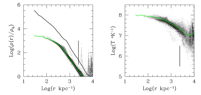
Figure 2: Density (left) and temperature (right) radial profiles for an SPH simulation of a galaxy cluster. The cluster has a virial mass of $7\times 10^{14}M_{\odot}$ and is resolved by roughly 12000 particles for each species. The force resolution is $25$ kpc. More details on the figure are given in the main text.

Following this recipe, one can write the fluid equations: mass conservation is automatically satisfied; one form of the Euler and energy equations is, in the adiabatic case⁷⁾:

$${d\vec{v}_{i}\over dt}=-\sum_{j=1}^{N}m_{j}\left[{p_{i}\over\rho_{i}^{2}}+{p_{j}\over\rho_{j}^{2}}\right]\vec{\nabla}_{i}W(|\vec{r}_{i}-\vec{r}_{j}|;h);$$ (12)

$${d\epsilon_{i}\over dt}={p_{i}\over\rho_{i}^{2}}\sum_{j=1}^{N}m_{j}(\vec{v}_{i}-\vec{v}_{j})\cdot\vec{\nabla}_{i}W(|\vec{r}_{i}-\vec{r}_{j}|;h).$$ (13)

Nonadiabatic terms are introduced in the same way; in particular, shock heating is allowed by adding artificial viscosity terms.

Hybrid methods have also been proposed¹⁰⁾, that make use of a grid to solve the fluid equations, but are Lagrangian in nature, since the grid itself is deformable and follows the fluid flow. The quite different approaches of Eulerian and Lagrangian methods, and the variety of codes within each approach, make it difficult to compare results coming from different codes, and to interpret the comparison. An attempt has however been done¹¹⁾ by evolving, from some high redshift to the present time, the same initial conditions of a cosmological model, using three different Eulerian codes and two different SPH codes; the results seem to indicate that Eulerian codes have better resolution on large scales and low $\rho$, low $T$ regions, while SPH codes can better resolve small scales and high $\rho$, high $T$ regions.

3 Applications: Formation of a galaxy cluster

Some results from an SPH simulation of a galaxy cluster are shown in Figure 2, as an example of application of the theory summarized in the previous Sections. The gas processes modeled are adiabatic heating and cooling, and viscous heating, while other cooling processes, photoionization and star formation were neglected, since they are not crucial to this particular problem.

The simulation has an Einstein-de Sitter background universe, with $H_{0}=50$ km s^-1 Mpc^-1, and with scale free power spectrum of perturbation $P(k)\propto k^{-1}$. The left panel shows the gas density (points), and the DM and gas mean density profiles (black and grey curve respectively), as a function of the distance $r$ from the cluster center; the vertical bar indicates the virial radius of the cluster. Note how the gas is less centrally concentrated than the DM. The density spikes in the gas profile are infalling substructure. The right panel shows the gas temperature and the mean temperature profile at different radii: the cluster is not isothermal, and its temperature drops by a factor of five from the center to the virial radius. During collapse the gas is shock heated to about $10^{7}$ - $10^{8}$ K as seen both in the main system and in the infalling substructures.

Acknowledgments

I would like to thank Bruno Guiderdoni for inviting me to give this talk. Thanks also to Bhuvnesh Jain, Ignasi Forcada and Simon White for comments on the manuscript. Financial support from an EC-HCM fellowship is gratefully acknowledged.

References

- [1] White, S.D.M., 1995, in ”Lecture Series of the Les Houches Summer School on ’Dark Matter and Cosmology’” August 1993, ed. R. Schaeffer, North Holland, in press.
- [2] Gunn, J.E. and Peterson, B.A., 1965, ApJ 142, 1633.
- [3] Rees, M.J. and Ostriker, J.P., 1977, MNRAS 179, 541.
- [4] Katz, N., Weinberg, D.H. and Hernquist, L., 1995, ApJS submitted.
- [5] Bryan, G. L., Norman, M. L., Stone, J. M., Cen, R., and Ostriker, J. P., 1995, Comp.Phys.Comm. 89, 149.
- [6] Ryu, D., Ostriker, J.P., Kang, H. and Cen, R., 1993, ApJ 414, 1.
- [7] Benz, W., 1990, in Numerical Modelling of Nonlinear Stellar Pulsations, ed. J.R. Buchler, Kluwer, Dordrecht.
- [8] Steinmetz, M., 1996, in Proceedings ”International School of Physics Enrico Fermi’”, Course CXXXII: Dark Matter in the Universe, Varenna 1995, IOP, in press.
- [9] Owen, M.O., Villumsen, J., Shapiro, P.R. and Martel, H., 1996, MNRAS sumbitted.
- [10] Gnedin, N.Y., 1995, ApJS 97, 231.
- [11] Kang, H. et al., 1994, ApJ 430, 83.