$\gamma$-ray emission and spectral evolution of pair plasmas in AGN jets

Abstract

The evolution of the particle distribution functions inside a relativistic jet containing an $e^{-}$-$e^{+}$pair plasma and of the resulting $\gamma$-ray and X-ray spectra is investigated. The first phase of this evolution is governed by heavy radiative energy losses. For this phase, approximative expressions for the energy-loss rates due to inverse-Compton scattering, using the full Klein-Nishina cross section, are given as one-dimensional integrals for both cooling by inverse-Compton scattering of synchrotron photons (SSC) and of accretion disk photons (EIC).

We calculate instantaneous and time-integrated $\gamma$-ray spectra emitted by such a jet for various sets of parameters, deducing some general implications on the observable broadband radiation. Finally, we present model fits to the broadband spectrum of Mrk 421. We find that the most plausible way to explain both the quiescent and the flaring state of Mrk 421 consists of a model where EIC and SSC dominate the observed spectrum in different frequency bands. In our model the flaring state is primarily related to an increase of the maximum Lorentz factor of the injected pairs.

1 Introduction

Accretion of matter onto a central black hole is the most relevant process to power active galactic nuclei (Lynden-Bell 1969, Salpeter 1969, Rees 1984). However, the details of the conversion processes of gravitational energy into observable electromagnetic radiation are still largely unknown. The discovery of many blazar-type AGNs (Hartman et al. 1992, Fichtel et al. 1993) as sources of high-energy gamma-ray radiation dominating the apparent luminosity, has revealed that the formation of relativistic jets and the acceleration of energetic charged particles, which generate nonthermal radiation, are key processes to understand the energy conversion process. Emission from relativistically moving sources is required to overcome gamma-ray transparency problems implied by the measured large luminosities and short time variabilities (for review see Dermer & Gehrels 1995).

Repeated gamma-ray observations of AGN sources have indicated a typical duty cycle of gamma-ray hard blazars of about 5 percent, supporting a “2-phase” model for the central regions of AGNs (Achatz et al. 1990, Schlickeiser & Achatz 1992). According to the 2-phase model the central powerhouse of AGNs undergoes two repeating phases: in a “quiescent phase” over most of the time ($\sim$95 percent) relativistic charged particles are efficiently accelerated in the central plasma near the black hole, whereas in a short and violent “flaring phase” the accelerated particles are ejected in the form of plasma blobs along an existing jet structure.

We consider the acceleration of charged particles during the quiescent phase. The central object accretes the surrounding matter. Associated with the accretion flow is low-frequency magnetohydrodynamic turbulence which is generated by various processes as e.g.:

(a) turbulence generated by the rotating accretion disk at large eddies and cascading to smaller scales (Galeev et al. 1979);

(b) stellar winds from solar-type stars in the central star cluster deliver plasma waves to the accretion flow;

(c) infalling neutral accretion matter becomes ionized by the ultraviolet and soft X-ray radiation of the disk. These pick-up ions in the accretion flow generate plasma waves by virtue of their streaming (Lee & Ip 1987);

(d) if standing shocks form in the neighbourhood of the central object they amplify any incoming upstream turbulence in the downstream accretion shock magnetosheath (McKenzie & Westphal 1969, Campeanu & Schlickeiser 1992).

These low-frequency MHD plasma waves from the accretion flow are the source of free energy and lead to stochastic acceleration of charged particles out of the thermal accretion plasma.

The dynamics of energetic charged particles (cosmic rays) in cosmic plasmas is determined by their mutual interaction and interactions with ambient electromagnetic, photon and matter fields. Among these by far quickest is the particle-wave interaction with electromagnetic fields, which very often can be separated into a leading field structure $F_{o}$ and superposed fluctuating fields $\delta F$. Theoretical descriptions of the transport and acceleration of cosmic rays in cosmic plasmas are usually based on transport equations which are derived from the Boltzmann-Vlasov equation into which the electromagnetic fields of the medium enter by the Lorentz force term. The quasilinear approach to wave-particle interaction is a second-order perturbation approach in the ratio $q_{L}\equiv({\delta F/F_{o}})^{2}$ and requires smallness of this ratio with respect to unity. In most cosmic plasmas this is well satisfied as has been established either by direct in-situ electromagnetic turbulence measurements in interplanetary plasmas, or by saturation effects in the growth of fluctuating fields. Nonlinear wave-wave interaction rates and/or nonlinear Landau damping set in only at appreciable levels of $(\delta F)^{2}$ and thus limit the value of $q_{L}\leq 1$. We assume the AGN plasma to have very high conductivity so that any large-scale steady electric fields are absent. We then consider the behaviour of energetic charged particles in a uniform magnetic field with superposed small-amplitude $(\delta B)^{2}\ll B_{o}^{2}$ plasma turbulence ($\delta\vec{E},\delta\vec{B}$) by calculating the quasilinear cosmic ray particle acceleration rates and transport parameters. This is by no means trivial since especially for the interaction of non-relativistic charged particles with ion- and electron-cyclotron waves thermal resonance broadening effects are particularly important (Schlickeiser & Achatz 1993, Schlickeiser 1994). The acceleration rates and spatial transport parameters are then used in the kinetic diffusion-convection equation for the isotropic part of the phase space density of charged particles $F(x,p,t)$ which for non-relativistic bulk speed $u\ll c$ reads

$${{\partial F}\over{\partial t}}-\,S_{o}={\partial\over{\partial x}}[\kappa{{\partial F}\over{\partial x}}]$$

$$\;\;\;-\,u{{\partial F}\over{\partial x}}+{p\over 3}{{\partial u}\over{\partial x}}{{\partial F}\over{\partial p}}+\,{1\over p^{2}}{\partial\over{\partial p}}[p^{2}A{{\partial F}\over{\partial p}}-p^{2}\dot{p}_{\rm loss}F].$$ (1)

Here $x$ denotes the spatial coordinate along the ordered magnetic field, $p$ the cosmic ray particle momentum, $\kappa$ is the spatial diffusion coefficient, $A$ the momentum diffusion coefficient, and $S_{o}$ denotes the ”Stossterm” describing the mutual interaction of the charged particles and their injection.

With respect to the generation of energetic charged particles, the basic transport equation (1) shows that stochastic acceleration of particles, characterized by the acceleration time scale $t_{A}=p^{2}/A$, competes with continuous energy loss processes $\dot{p}_{\rm loss}$, characterized by energy loss time scales $t_{L}=p/|\dot{p}_{\rm loss}|$. Dermer et al. (1996) have recently inspected the acceleration of energetic electrons and protons in the central AGN plasma by comparing the time scales for stochastic acceleration with the relevant energy loss time scales. At small proton momenta the Coulomb loss time scale is extremely sensitive to the background plasma density and temperature, and for slight changes in the values of these parameters cosmic ray protons may not be accelerated above the Coulomb barrier. Although at small particle momenta the plasma wave’s dissipation and the interaction with the cyclotron waves become decisive and might modify the acceleration time significantly, the results of Dermer et al. (1996) demonstrate that reasonable central AGN plasma parameter values are possible where the low-frequency turbulence energizes protons to TeV and PeV energies where photo-pair and photo-pion production are effective in halting the acceleration (Sikora et al. 1987, Mannheim & Biermann 1992). According to the results of Dermer et al. (1996) it takes about $\simeq 10M_{8}$ days for the protons to reach these energies, where $M_{8}$ is the mass of the central black hole in units of $10^{8}\,M_{\odot}$. The corresponding analysis for cosmic ray electrons shows that the external compactness provided by the accretion disk photons (Becker & Kafatos 1995) leads to heavy inverse Compton losses which suppress the acceleration of low-energy electrons beyond Lorentz factors of $\gamma\approx 10-100$. It seems that due to their much smaller radiation loss rate cosmic ray protons are effectively accelerated during the quiescent phase in contrast to low energy electrons.

Now an important point has to be emphasized: once the accelerated protons reach the thresholds for photo-pair ($\gamma_{p,th}=m_{e}c^{2}/<\epsilon>=5\cdot 10^{4}\epsilon^{-1}_{1}$) and photo-pion production and the threshold for pion production in inelastic proton-matter collisions they will generate plenty of secondary electrons and positrons of ultrahigh energy which are now injected at high energies ($E_{s}\geq 25{\rm GeV}\epsilon^{-1}_{1}$) into this acceleration scheme. $<\epsilon>=10\epsilon_{1}$ eV denotes the mean accretion disk photon energy. It is now of considerable interest to follow the evolution of these injected secondary particles.

Although many details of this evolution are poorly understood, it is evident that the further fate of the secondary particles depends strongly on whether they find themselves in a compact environment set up by the external accretion disk, or not. As has been pointed out by Dermer & Schlickeiser (1993b) as well as Becker & Kafatos (1995) the size of the gamma-ray photosphere (where the compactness is greater unity so that any produced gamma-ray photon is pair-absorbed) is strongly photon energy dependent. The gamma-ray photosphere attains its largest size at photon energies $E_{p}\simeq 50\epsilon_{1}^{-1}$ GeV. Secondary particles within the photosphere having energies $E_{s}\leq E_{p}$ will initiate a rapid electromagnetic cascade which has been studied by e.g. Mastichiadis & Kirk (1995), which might even lead to runaway pair production and associated strong X-ray flares (Kirk & Mastichiadis 1992), and/or due to the violent effect of a pair catastrophy (Henri & Pelletier 1993) ultimately lead to an explosive event and the emergence of a relativistically moving component filled with energetic electron-positron pairs.

In contrast, if the secondary particles are generated outside the gamma-ray photosphere the secondary electrons and positrons will quickly cool by the strong inverse Compton losses generating plenty of gamma-ray emission up to TeV energies. As solutions of the electron and positron transport equation (1) for this case demonstrate (Schlickeiser 1984, Pohl et al. 1992) a cooling particle distribution ($N(p)\propto p^{-2}$) with a strong cutoff at low (but still relativistic) momentum $p_{c}$ develops, which grows with time as more and more protons hit the photo-pair and photo-pion thresholds. Such bump-on-tail particle distribution functions, which are inverted ($\partial F/\partial p>0$) below $p_{c}$, are collectively unstable with respect to the excitation of electromagnetic and electrostatic waves such as oblique longitudinal Langmuir waves (Lesch et al. 1989). As described in detail by Lesch & Schlickeiser (1987) and Achatz et al. (1990), depending on the local plasma parameters (mainly the electron temperature of the background gas and the density ratio $N_{o}/n_{e}$ of relativistic electrons and positrons to thermal electrons) these Langmuir waves either (1) lead to quasilinear plateauing of the inverted distribution function and rapid collective thermalization of the electrons and positrons, or (2) are first damped by nonlinear Landau damping, but ultimately heat the background plasma strongly via the modulation instability once a critical energy density in Langmuir waves $W_{c}=n_{e}(k_{B}T_{e}/m_{e}c^{2})^{2}$ has been built up. Both relaxation mechanisms terminate the quiescent phase of the acceleration process. The almost instantaneous increase of the background gas entropy due to the rapid modulation instability heating again leads to an explosive outward motion of the plasma blob carrying the relativistic particles away from the central object.

As we have discussed, in both cases it is very likely that at the end of the quiescent phase an explosive event occurs that gives rise to the emergence of a new relativistically moving component filled with energetic electron-positron pairs. It marks the start of the flaring phase in gamma-ray blazars. The initial starting height of the emerging blob $z_{i}$ entering the calculation of the gamma-ray flux should be closely related to the size of the acceleration volume in the quiescent phase mainly determined by the maximum size of the gamma-ray photosphere. This scenario is supported by the measurements of Babadzanhanyants & Belokon (1985) that in 3C 345 and other quasars optical bursts are in close time correlation with the generation of compact radio jets. A similar behaviour has also been observed during the recent simultaneous multiwavelength campaign on 3C 279 (Hartman et al. 1996). Further corroborative evidence for this scenario is provided by the recent discovery of superluminal motion components in the gamma-ray blazars PKS 0528+134 (Pohl et al. 1995) and PKS 1633+382 (Barthel et al. 1995) that demonstrate a close physical connection between gamma-ray flaring and the ejection of new superluminal jet components in blazars.

It is the purpose of the present investigation to follow the time evolution of the relativistic electrons and positrons as the emerging relativistic blob moves out. Because of the very short radiative energy loss time scales of the radiating electrons and positrons it is important to treat the spectral evolution of the radiating particles self-consistently. In earlier work Dermer & Schlickeiser (1993a) and Dermer et al. (1997) have studied the spectral time evolution from a modified Kardashev (1962) approach by injecting instantaneously a power law electron and positron energy spectrum at height $z_{i}$ at the beginning of the flare, and calculating its modification with height in the relativistically outflowing blob due to the operation of various continous energy loss processes as inverse Compton scattering, synchrotron radiation, nonthermal bremsstrahlung emission and Coulomb energy losses. Here we generalize their approach by accounting for Klein-Nishina effects and including as well external inverse-Compton scattering as synchrotron self-Compton scattering self-consistently.

The acceleration scenario described above leads us to the following assumptions on the distribution of pairs inside a new jet component at the time of their injection: If the pairs are created by photo-pair production, their minimum Lorentz factor is expected to be in the range of the threshold value of the protons’ Lorentz factor for photo-pair production. We use the standard accretion disk model by Shakura & Sunyaev (1973), which we will describe in more detail in the next section, to fix this threshold, determined by the average disk photon energy $\langle\epsilon\rangle$. The pair distribution above this cutoff basically reflects the acceleration spectrum of the protons, i. e. a power-law distribution with spectral index $2\lower 4.0pt\hbox{$\buildrel<\over{\sim}$}s\lower 4.0pt\hbox{$\buildrel<\over{\sim}$}3$ ($n(\gamma)\sim\gamma^{-s}$) which extends up to $\gamma_{2\pm}\sim 10^{6}$. This yields the initial pair distribution functions

f_± (γ_±) = γ_±^-σ                  γ_1±≤γ_±≤γ_2±

(2)

with $4\lower 4.0pt\hbox{$\buildrel<\over{\sim}$}\sigma\lower 4.0pt\hbox{$\buildrel<\over{\sim}$}5$. The differential number of particles in the energy intervall $[\gamma_{\pm},\gamma_{\pm}+d\gamma_{\pm}]$ per unit volume is then given by

$$d\,n_{\pm}=4\,\pi\,N_{\pm}\,\gamma_{\pm}^{2}\beta_{\pm}\,f_{\pm}(\gamma_{\pm})d\gamma_{\pm}$$ (3)

where $N_{\pm}$ is a normalization factor related to the total particle density $n_{\pm}$ through $N_{\pm}\approx n_{\pm}{\sigma-3\over 4\,\pi}\gamma_{1\pm}^{\sigma-3}$.

The detection of TeV $\gamma$-rays from Mrk 421 suggests that such components must be produced/accelerated outisde the $\gamma$-ray photosphere for photons of energy $\sim 1$ TeV. The height of this photosphere due to the interaction of $\gamma$-rays with accretion disk radiation will be determined self-consistently in section 4. Backscattering of accretion disk radiation by surrounding clouds is negligible in the case of BL Lac objects emitting TeV $\gamma$-rays (Böttcher & Dermer, 1995).

We point out that most of our basic conclusions are also valid if the pairs inside the blob are accelerated by other mechanisms, e. g. by a relativistic shock propagating through the jet.

Beginning at the injection height (henceforth denoted as $z_{i}$), we follow the further evolution of the pair distribution and calculate the emerging photon spectra.

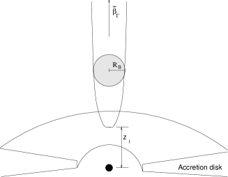
Figure 1: Model for the geometry of a relativistic AGN jet

The negligibility of pair absorption due to the interaction with the synchrotron and $\gamma$-ray emission from the jet is checked self-consistently during our calculations.

Interactions of the jet pair plasma with dilute surrounding material will cause turbulent Alfvén and Whistler waves. It has been shown by Achatz & Schlickeiser (1993) that a low-density, relativistic pair jet is rapidly disrupted as a consequence of the excitation of such waves. Thus, to insure stability of the beam over a sufficient length scale, we need that the density of pairs inside the jet exceeds the density of the surrounding material. In this case, pitch angle scattering on plasma wave turbulences leads to an efficient isotropization of the momenta of the pairs in the jet without destroying the jet structure. Thus, additional assumptions on our initial conditions are that the particle momenta are isotropically distributed in the rest frame of a new jet component (blob) and that the density of pairs in the jet $n_{j}\gg n_{b}$ where $n_{b}$ is the density of the background material.

This study is devided into two papers. In the first (present) paper we investigate the details of electron/positron cooling due to inverse-Compton scattering and follow the pair distribution and photon spectra evolution during the first phase in which the system is dominated by heavy radiative losses. In the second paper we will consider the later phase of the evolution where collisional effects (possibly leading to thermalization) and reacceleration become important, and a plausible model for MeV blazars which follows directly from our treatment will be presented (Böttcher, Pohl & Schlickeiser, in prep.).

In section 2 of this first paper, we describe in detail how to calculate the energy-loss rates due to the various processes which we take into account and give useful approximative expressions for the inverse-Compton losses (as well scattering of accretion disk radiation as of synchrotron radiation), including all Klein-Nishina effects. In section 3, we discuss the relative importance of the various processes. The location of the $\gamma$-ray photosphere for TeV $\gamma$-rays is briefly outlined in section 4. The technique used to follow the evolution of the pair distributions is described in section 5. In section 6, we describe how to use the pair distributions resulting from our simulations in order to calculate the emanating $\gamma$-ray spectra, and in section 7 we discuss general results of our simulations giving a prediction for GeV – TeV emission from $\gamma$-ray blazars which due to the lack of sensitivity of present-day instruments in this energy range could not be observed until now. Only two extragalactic objects have been detected as sources of TeV emission, namely Mrk 421 (Punch et al. 1992) and Mrk 501 (Quinn et al. 1995). In Section 8, we use our code to fit the observational results on the broadband emission during the TeV flare of Mrk 421 in May 1994 and on its quiescent flux. We summarize in section 9.

2 Energy-loss rates

We first consider in detail the various processes through which the pairs inside a new AGN jet component lose energy. The blob is assumed to move outward perpendicularly to the accretion disk plane with velocity $c\,\beta_{\Gamma}=c\,\sqrt{1-1/\Gamma^{2}}$ where $\Gamma$ is the Lorentz factor of the bulk motion. The mechanisms that we take into account are inverse-Compton scattering of accretion disk photons, synchrotron and synchrotron-self-Compton (SSC) losses. It is well-known that energy exchange/loss due to elastic (Møller and Bhabha scattering) and inelastic scattering (pair bremsstrahlung emission) do not contribute significantly for ultrarelativistic particles. We consider them in detail in the second paper of this series, dealing with mildly-relativistic pair plasmas. The same is true for pair annihilation losses.

2.1 External inverse-Compton losses

We are now considering the single-particle energy loss rate due to inverse-Compton scattering of external photons coming directly from a central source, which we assume to be an accretion disk. We use the accretion disk model of Shakura & Sunyaev (1973) predicting, for a central black hole of $M\sim 10^{6}$ – $10^{8}\,M_{\odot}$, a blackbody spectrum according to a temperature distribution $T(R)$ given by

$$\Theta(R)={k_{b}\,T(R)\over m_{e}c^{2}}=1.44\,\left({M\over M_{\odot}}\right)^{-{1\over 2}}\,\cdot$$

$$\;\;\;\;\;\;\cdot\,\left({\dot{M}\over M_{\odot}/{\rm yr}}\right)^{1\over 4}\,\left({R\over R_{g}}\right)^{-{3\over 4}}\,\left(1-\sqrt{6\,R_{g}\over R}\right)^{1\over 4}.$$ (4)

In general, the energy loss rate due to inverse-Compton scattering is given by the manifold integral

$$-\left({d\gamma\over dt}\right)_{IC}={c\over 2}\int\limits_{-1}^{1}d\eta_{e}\>\int\limits_{-1}^{1}d\eta_{ph}\int\limits_{0}^{2\pi}d\phi\int\limits_{0}^{\infty}d\epsilon\int\limits_{-1}^{1}d\kappa^{\prime}\int\limits_{0}^{2\pi}d\phi_{s}^{\prime}$$

$$\int\limits_{0}^{\infty}d\epsilon_{s}^{\prime}(1-\beta\mu){d\sigma_{KN}\over d\epsilon_{s}^{\prime}\,d\Omega_{ph,s}^{\prime}}\>n_{ph}(\epsilon,\Omega_{ph})\,\Bigl{(}\gamma\,\epsilon_{s}^{\prime}\,[1+\beta\mu_{s}^{\prime}]-\epsilon\Bigr{)}$$ (5)

where $\eta_{e}=\cos\theta_{e}$, $\eta_{ph}=\cos\theta_{ph}$, $\kappa^{\prime}=\cos\chi^{\prime}$,

Figure 2: Definition of the angles for calculation of the inverse-Compton losses. ’L’ in the right panel denotes the motion of the labor frame with respect to the electron rest frame. The subscript ‘ph’ refers to quantities of the photon

$$\mu=\cos\psi=\eta_{ph}\,\eta_{e}+\sin\theta_{ph}\,\sin\theta_{e}\,\cos\phi$$ (6)

$$\mu_{s}^{\prime}=\cos\psi_{s}^{\prime}=\kappa^{\prime}\,\mu^{\prime}+\sin\chi^{\prime}\,\sin\psi^{\prime}\,\cos\phi_{s}^{\prime}.$$ (7)

Here, primed quantities refer to the rest frame of the electron, and the subscript ’s’ denotes quantities of the scattered photon. The definition of the angles is illustrated in Fig. 2. Now, let the superscript ’$\ast$’ denote quantities measured in the rest frame of the accretion disk. Then, the differential number of accretion disk photons in the blob frame is

$${dn_{ph}\over d\epsilon d\Omega_{ph}}={\epsilon^{2}\over\epsilon^{\ast\,2}}\left({dn_{ph}\over d\epsilon d\Omega_{ph}}\right)^{\ast}=$$

$${1\over 2\,c^{3}}\left({m_{e}c^{2}\over h}\right)^{3}\,\epsilon^{2}\left(e^{\epsilon{\Gamma(1+\beta_{\Gamma}\eta_{ph})\over\Theta(R)}}-1\right)^{-1}\>{1+\beta_{\Gamma}\eta_{ph}\over\eta_{ph}+\beta_{\Gamma}}.$$ (8)

Using this photon number and the full Klein-Nishina cross section, Eq. (5) becomes

$$-\left({d\gamma\over dt}\right)_{IC}={\pi r_{e}^{2}\,\Gamma^{2}\over 4\,z^{2}\,c^{2}}\left({m_{e}c^{2}\over h}\right)^{3}\int\limits_{-1}^{1}d\eta_{e}\int\limits_{R_{\rm min}}^{R_{\rm max}}R\,dR\int\limits_{0}^{2\pi}d\phi$$

$$\int\limits_{0}^{\infty}d\epsilon\>\epsilon^{3}\left(e^{\epsilon{\Gamma(1+\beta_{\Gamma}\eta_{ph})\over\Theta(R)}}-1\right)^{-1}\int\limits_{-1}^{1}d\kappa\>(1-\beta\mu)\left(\eta_{ph}+\beta_{\Gamma}\right)^{2}\,\cdot$$

$${1+F\,(F-1)+F\,{\kappa^{\prime}}^{2}\over F^{3}}\left(\gamma^{2}{1-\beta\mu+\beta\,\kappa^{\prime}[\mu-\beta]\over F}-1\right)$$ (9)

where

$$F=1+\epsilon\,\gamma(1-\beta\mu)\,(1-\kappa^{\prime}),$$ (10)

$$\eta_{ph}={z-\beta_{\Gamma}\,\sqrt{R^{2}+z^{2}}\over\sqrt{R^{2}+z^{2}}-\beta_{\Gamma}\,z}$$ (11)

and $R_{\rm min}$ and $R_{\rm max}$ are the radius of the inner and outer edge of the accretion disk, respectively.

If all scattering occurs in the Thomson regime ($F\equiv 1$), we find (neglecting terms of order $1/\gamma^{2}$):

$$-\left({d\gamma\over dt}\right)_{IC}\>\approx\>{4\over 45}\gamma^{2}{\pi^{5}\,\sigma_{T}\over c^{2}}\,\Gamma^{2}\,\left({m_{e}c^{2}\over h}\right)^{3}\,\cdot$$

$$\;\;\;\;\;\;\;\;\;\;\int\limits_{R_{\rm min}}^{R_{\rm max}}dR\,R\,\Theta^{4}(R)\,{\left(x-\beta_{\Gamma}\,z\right)^{2}\over x^{4}}$$ (12)

where $x=\sqrt{R^{2}+z^{2}}$. Fig. 3 shows the energy loss rate computed using the full Klein-Nishina cross-section compared to the calculation in the Thomson limit as quoted above as well as the calculation in the Thomson limit, combined with a point-source approximation for the accretion disk (e. g. Dermer & Schlickeiser 1993).

Figure 3: Energy loss rates of a test electron/positron due to inverse-Compton scattering of accretion disk photons. Total disk luminosity: $L_{0}=10^{44}$ erg s^-1, height: $z=2\cdot 10^{-4}$ pc

For electron energies of $\gamma\ll\Gamma/\langle\epsilon_{disk}\rangle$, Eq. (12) is a very good approach to the Inverse-Compton losses. In the case of small distances to the accretion disk ($z\lower 4.0pt\hbox{$\buildrel<\over{\sim}$}10^{-2}$ pc in the case of a disk luminosity $L_{0}=10^{46}$ erg s^-1; $z\lower 4.0pt\hbox{$\buildrel<\over{\sim}$}10^{-3}$ pc for $L_{0}=10^{44}$ erg s^-1) the point-source approximation is not an appropriate choice.

A very useful approximation for all electron energies is based on replacing the integration ${1\over 2}\int_{-1}^{1}d\eta_{e}$ by setting $\eta_{e}=0$. Furthermore, one can approximate the thermal spectrum, emitted by each radius of the disk, by a $\delta$ function in energy, $n(\epsilon,\Omega)\approx A\,\delta(\epsilon-<\epsilon>[R])$ where

$$<\epsilon>(R)={\Gamma(4)\zeta(4)\over\Gamma(3)\zeta(3)}{\Theta(R)\over\Gamma(1+\beta_{\Gamma}\eta_{ph})}.$$

With these simplifications, and neglecting terms of order $1/\gamma^{2}\ll 1$, Eq. (9) becomes

$$-\left({d\gamma\over dt}\right)_{IC}=\gamma^{2}{\pi^{5}\sigma_{T}\,\Gamma^{2}\over 40\,c^{2}}\left({m_{e}c^{2}\over h}\right)^{3}\int\limits_{R_{min}}^{R_{max}}R\,dR\,\cdot$$

$$\;\;\;\;\cdot\,\Theta(R)^{4}{R\,(x-\beta_{\Gamma}z)^{2}\over x^{4}}\,I(<\epsilon>,\gamma,\eta_{ph})$$ (13)

where

$$I(\epsilon,\gamma,\eta_{ph}):=\int\limits_{0}^{2\pi}d\phi\>(1-\beta\mu)^{2}\,\cdot$$

$$\;\;\;\;\;\;\cdot\,\int\limits_{-1}^{1}d\kappa^{\prime}\>(1-\kappa^{\prime})\,{1+F^{2}+F\,(\kappa^{\prime 2}-1)\over F^{4}}$$ (14)

and

$$\mu=\sqrt{1-\eta_{ph}^{2}}\,\cos\phi$$

$$F=1+E\,(1-a\,\cos\phi)\,(1-\kappa^{\prime})$$

$$E=\epsilon\gamma,$$

$$a=\beta\sqrt{1-\eta_{ph}^{2}}.$$

The integral $I$ can be solved analytically, yielding

$$I(\epsilon,\gamma,\epsilon_{ph})={2\,\pi\over E^{2}}\Biggl{\{}{6\over E\,\sqrt{1-a^{2}}}-{5\over 6}+\ln\left({1+2\,E+N\over 2}\right)$$

$$-{2\over E}\,{\ln\left({E\,a\over A}\right)\over\sqrt{1-a^{2}}}-{8\,D\over E\,a}\,{\ln(1-A\,D)\over 1-D^{2}}-{3\over E^{2}}\,{\ln\left({E\,a\over A}\right)\over(1-a^{2})^{3/2}}$$

$$-{24\,D^{2}\over E^{2}\,a^{2}\,(1-D^{2})^{2}}\left({1+D^{2}\over 1-D^{2}}\,\ln[1-A\,D]-{A\,D\over 1-A\,D}\right)$$

$$\;\;\;\;\;+{2\,(1+2\,E)^{2}+(2\,E\,a)^{2}\over 6\>N^{5}}-{1+2\,E\over 2\,N^{3}}-{1\over N}\Biggr{\}}$$ (15)

where

$$N=\sqrt{(1+2\,E)^{2}-(2\,E\,a)^{2}},$$

$$A={1+2\,E\over 2\,E\,a}-\sqrt{\left({1+2\,E\over 2\,E\,a}\right)^{2}-1}\><\>1,$$

$$D={1\over a}-\sqrt{{1\over a^{2}}-1}\><\>1.$$

For small values of $E$, one should use the Taylor expansion of Eq. (15), namely

$$I(\epsilon,\gamma,\epsilon_{ph})\Bigr{|}_{E<{1\over 2}}=2\,\pi\,\Biggr{\{}{8\over 3}\,\left(1+{a^{2}\over 2}\right)$$

$$-{56\over 5}\,E\,\left(1+{3\over 2}\,a^{2}\right)+{92\over 5}\,E^{2}\,\left(1+3\,a^{2}+a^{4}\right)\Biggr{\}}+o\Bigl{(}E^{3}\Bigr{)}.$$ (16)

This result (using Eq. [16] for $E<0.05$) is illustrated by the dot-dashed curve in Fig. 3. In Fig. 5, the inverse-Compton losses (according to Eq. [13]) for set of parameters which is assumed to be typical for BL Lac objects ($L_{0}=10^{44}{\rm erg\,s}^{-1}$, $z=2\cdot 10^{-4}$ pc, $\Gamma=10$) are compared to the synchrotron and SSC energy losses derived in the following subsections.

2.2 Synchrotron and synchrotron-self-Compton losses

If, for the synchrotron (sy) losses, we neglect inhomogeneities and effects of anisotropy, we have

$$\left({d\gamma\over dt}\right)_{sy}=-{4\over 3}c\,\sigma_{T}{B^{2}\over 8\pi m_{e}c^{2}}(\gamma_{t}^{2}-1)$$

$$\hskip 71.13188pt\approx-\,3.25\cdot 10^{-8}\;B_{0}^{2}\>\gamma_{t}^{2}\;{\rm s}^{-1}$$ (17)

(e. g., Rybicki & Lightmann 1979) where $B_{0}:=B/(1\,{\rm G})$.

Evaluating the single-particle energy loss rate due to the SSC process, we restrict ourselves to regarding only single scattering events. If the particle distribution functions are given by power-laws, the synchrotron photon spectrum is also described by a power-law. However, since we are intrested in the detailed shape of the distributions, deviating from a simple power-law, we have to calculate the synchrotron spectrum in more detail.

In an optically thin source, the differential number of synchrotron photons in the energy interval $[\epsilon,\epsilon+d\epsilon]$ is given by

$$n_{sy}(\epsilon)=$$

$$\;\;\;\;\;\;\;{R_{B}\over 3\,\,c}\,{m_{e}c^{2}\over h}\sum\limits_{\pm}\int\limits_{1}^{\infty}d\gamma_{\pm}\>{P_{\nu}(\gamma_{\pm})\over h\,\nu}\Biggr{|}_{\nu=\epsilon\,{m_{e}c^{2}\over h}}\>n_{\pm}(\gamma_{\pm}).$$ (18)

The summation symbol denotes the sum of the contributions from electrons and positrons to the synchrotron spectrum. Averaging over all pitch-angles of the electrons, the spectral emissivity $P_{\nu}(\gamma)$ of a single electron of Lorentz factor $\gamma$ can be expressed as

$${P_{\nu}(\gamma)\over h\,\nu}={\alpha\,\pi\over\sqrt{3}\,\gamma^{2}}\,\left(1+\left[\gamma{\nu_{p}\over\nu}\right]^{2}\right)\,CS(x)$$ (19)

(Crusius & Schlickeiser 1986) where $\alpha$ is the finestructure constant,

$$x={2\,\nu\over 3\,\nu_{e}\,\gamma^{2}}\,\left(1+\left[\gamma{\nu_{p}\over\nu}\right]^{2}\right)^{3\over 2},$$ (20)

$\nu_{e}$ is the non-relativistic electron/positron gyrofrequency, $\nu_{p}$ is the plasma frequency of the relativistic pair plasma, i. e.

$$\nu_{p}=\sqrt{n_{e}\,e^{2}\over\pi\,m_{e}\,\langle\gamma\rangle}$$ (21)

$$CS(x)=W_{0,{4\over 3}}(x)\,W_{0,{1\over 3}}(x)\>-\>W_{{1\over 2},{5\over 6}}(x)\,W_{-{1\over 2},{5\over 6}}(x)$$ (22)

and $W_{\kappa,\mu}$ are the Whittaker functions.

If the particle density exceeds $n\lower 4.0pt\hbox{$\buildrel>\over{\sim}$}10^{8}$ cm^-3 synchrotron self absorption (SSA) is negligible for the following two reasons: The optical depth due to synchrotron self absorption for an initial power-law distribution $n(\gamma)=n_{0}\,\gamma^{-2}$ can be estimated as

$$\tau_{\rm SSA}\approx{\sqrt{3}\,\alpha\,\hbar\,c^{2}\over m_{e}c^{2}}\,\Gamma\left({5\over 3}\right)\,\Gamma\left({4\over 3}\right)\,n_{0}\,\nu_{e}^{2}\,\nu^{-3}\,R_{B}$$ (23)

(Schlickeiser & Crusius 1989). This optical depth becomes unity for

$$\nu_{\rm SSA}=5.7\cdot 10^{10}\>\gamma_{1;3}^{1/3}\,B_{-1}^{2/3}\,n_{9}^{1/3}\,R_{11}^{1/3}\;{\rm Hz}$$ (24)

where $\gamma_{1;3}$ is the lower cutoff Lorentz factor in units of $10^{3}$, $B_{-1}$ is the magnetic field in units of $0.1$ G, $n_{9}$ is the pair density in units of $10^{9}$ cm^-3 and $R_{11}$ is the blob radius in units of $10^{11}$ cm. The frequency $\nu_{\rm SSA}$ is of the same order as the Razin-Tsytovich frequency

$$\nu_{R}=2\cdot 10^{11}\>n_{9}\,B_{-1}^{-1}\,\langle\gamma\rangle^{-1/2}\;{\rm s}^{-1}$$ (25)

where the luminosity is strongly suppressed due to plasma effects. Here, $\langle\gamma\rangle$ denotes the average electron Lorentz factor. This demonstrates that for pair densities $n\lower 4.0pt\hbox{$\buildrel>\over{\sim}$}10^{8}$ cm^-3 synchrotron self absorption can be neglected. For lower densities we include it in our calculations, evaluating

$$\tau_{\rm SSA}=-R_{B}{c^{2}\over 8\pi\nu^{2}m_{e}c^{2}}\int\limits_{1}^{\infty}d\gamma\>P_{\nu}(\gamma)\,\gamma^{2}{d\over d\gamma}\left({n[\gamma]\over\gamma^{2}}\right)$$ (26)

(e. g., Rybicki & Lightman, 1979) self-consistently.

From the point of view of reacceleration, synchrotron self absorption can be neglected since particles resonating with photons at the lower cut-off of the synchrotron spectrum should have Lorentz factors of

$$\gamma_{res}\approx 450\>\gamma_{1;3}^{1/6}\,B_{-1}^{-1/6}\,n_{9}^{1/6}\,R_{11}^{1/6}$$ (27)

which is lower than the particle Lorentz factors we deal with in the simulations carried out in this paper.

If all scattering occurs in the Thomson limit, $\gamma_{\pm}\,\epsilon\ll 1$, the first order SSC energy loss rate is easily determined by

$$\left({d\gamma_{t}\over dt}\right)_{\rm SSC}=-{4\over 3}c\,\sigma_{T}\,\left(\gamma_{\pm}^{2}-1\right)\int\limits_{0}^{\infty}d\epsilon\>\epsilon\>n_{sy}(\epsilon).$$ (28)

where the synchrotron luminosity can be calculated as

$$\int\limits_{0}^{\infty}d\epsilon\>\epsilon\,n_{sy}(\epsilon)={R_{B}\over 3\,c}\int\limits_{1}^{\infty}d\gamma_{\pm}n_{\pm}(\gamma_{\pm})\,\left|\left({d\gamma_{\pm}\over dt}\right)_{sy}\right|,$$ (29)

yielding for the initial power-law distribution functions

$$\left({d\gamma_{t}\over dt}\right)_{\rm SSC}\approx$$

$${16\over 27}c\,\sigma_{T}^{2}\left({B^{2}\over 8\pi\,m_{e}c^{2}}\right)R_{B}\,n_{\pm}\,\gamma_{2\pm}^{3-s}\gamma_{1\pm}^{s-1}\,{s-1\over 3-s}\>\gamma^{2}.$$ (30)

Discarding the Thomson approximation and using the notation of the previous subsection, the exact expression for the SSC energy losses is

$$-\left({d\gamma\over dt}\right)_{\rm SSC}={c\,\pi\,r_{e}^{2}\over 2}\int\limits_{-1}^{1}d\mu\int\limits_{-1}^{1}d\kappa^{\prime}\int\limits_{0}^{\infty}d\epsilon\>\epsilon\,n_{ph}(\epsilon)\,(1-\beta\mu)\,\cdot$$

$$\cdot\,{1+F\,(F-1)+F\,{\kappa^{\prime}}^{2}\over F^{3}}\left(\gamma^{2}{1-\beta\mu+\beta\kappa^{\prime}\,[\mu-\beta]\over F}-1\right).$$ (31)

Figure 4: Energy loss rates of a test electron/positron due to inverse-Compton scattering of synchrotron photons. $B=1$ G, $R_{B}=10^{15}$ cm, $n_{e}=10^{4}$ cm^-3. Thomson-scattering (dotted curves) and exact Klein-Nishina cross-section (solid curves)

In this case of an isotropic radiation field in the blob frame, the integrations over $\mu$ and $\kappa^{\prime}$ can be solved analytically if we neglect terms of order $1/\gamma^{2}\ll 1$ and of order $\epsilon/\gamma\ll 1$. This yields

$$-\left({d\gamma\over dt}\right)_{\rm SSC}=c\,\pi\,r_{e}^{2}\int\limits_{0}^{\infty}d\epsilon\>n_{ph}(\epsilon)\>{G(\gamma\epsilon)\over\epsilon},$$ (32)

where $c\,\pi\,r_{e}^{2}\,G(\gamma\epsilon)/\epsilon$ cm^-3 is the energy loss rate of an electron of energy $\gamma$ scattering an isotropic, monochromatic radiation field of photon energy $\epsilon$ and photon density 1 cm^-3 and

$$G(E)={8\over 3}\,E\,{1+5\,E\over(1+4\,E)^{2}}-{4\,E\over 1+4\,E}\left({2\over 3}+{1\over 2\,E}+{1\over 8\,E^{2}}\right)$$

$$+\ln(1+4\,E)\left(1+{3\over E}+{3\over 4}\,{1\over E^{2}}+{\ln[1+4\,E]\over 2\,E}-{\ln[4\,E]\over E}\right)$$

$$\;\;\;\;\;\;\;\;\;\;\;-{5\over 2}{1\over E}+{1\over E}\sum\limits_{n=1}^{\infty}{(1+4\,E)^{-n}\over n^{2}}-{\pi^{2}\over 6\,E}-2.$$ (33)

For small values of $E=\gamma\epsilon$ (i. e. the Thomson limit) the Taylor expansion

$$G(E)\biggr{|}_{E<{1\over 4}}=E^{2}\,\left\{{32\over 9}-{112\over 5}E+{3136\over 25}E^{2}+o\bigl{(}E^{3}\bigr{)}\right\}$$ (34)

to lowest order reduces Eq. (32) to Eq. (28) for $\gamma^{2}\gg 1$. In Fig. 4, the analytic solution (32) is compared to the Thomson scattering result (Eq. [27]).

Figure 5: Energy loss rates of a test particle (Lorentz factor $\gamma_{t}$) due to inverse-Compton scattering of external (accretion disk) photons (EIC; disk luminosity $L_{0}=10^{44}{\rm erg\,s}^{-1}$, $M_{BH}=10^{6}\,M_{\odot}$, $z=2\cdot 10^{-4}$ pc, $\Gamma=10$) and of synchrotron photons (SSC; $B=1$ G, $R_{B}=10^{15}$ cm, $n_{\pm}=10^{4}$ cm^-3, $\sigma=4.0$), and to synchrotron emission ($B=1\,G$)

It should be noted that for such an ultrarelativistic particle distribution Compton scattering its own synchrotron photons, Klein-Nishina corrections do not lead to a break in the energy dependence of the energy-loss rate, but due to the fact that with increasing energy a decreasing fraction of the scattering events occurs in the Thomson regime, lead to a much smoother flattening of the energy depencence than what is obtained from the relatively sharp soft photon distribution coming from the accretion disk. In the energy regime considered here, the energy-loss rate scales as $-d\gamma/dt\,\sim\,\gamma^{\alpha}$ with $\alpha\approx 1.5$ for the spectral index $s\sim 2$ of the particle distributions $n(\gamma)\sim\gamma^{-s}$. Clearly, this effect depends strongly on the temporal particle distribution which determines the synchrotron spectrum.

The result of Eq. (32) (using Eq. [34] for $E<0.1$) is included in Fig. 5 for a magnetic field strength of ${\rm B}=\,1$ G and a blob radius of $R_{B}=10^{15}$ cm. Higher-order SSC scattering (up to $n$th order in the $n$th time step) is incorporated in our simulations by replacing $n_{sy}(\epsilon)$ by $n_{sy}(\epsilon)+n_{\rm SSC}(\epsilon)$ in Eq. (32).

3 Discussion of the elementary processes

From Fig. 5 we can deduce some estimates about which of the various energy loss and exchange processes discussed above play an important role in different energy regimes of particles.

First, we note that the energy transfer rates due to collisional effects (elastic scattering, bremsstrahlung emission) and the pair annihilation rate scale linearly with particle density $n$. The synchrotron and SSC losses basically scale as $\sim B^{2}$ (the SSC losses, additionally, $\sim R_{B}\cdot n$), whereas the external inverse-Compton losses basically scale as $L_{0}\,/\,z^{2}$. The SSC losses also strongly depend on the steepness of the initial distribution functions since a harder particle spectrum yields a harder synchrotron spectrum which, in turn, leads to higher inverse-Compton losses.

The effect of elastic scattering is of minor importance for ultrarelativistic particles. We find the time-scale for thermalization to be given by

$$\tau_{\rm th}:={\gamma_{t}-1\over\left|d\gamma_{t}/dt\right|_{\rm elast.\,scat.}}\approx{2.5\cdot 10^{12}\over n_{4}}\>{\rm s}$$ (35)

for $\gamma_{t}=100$ which increases rapidly towards higher particle energies. Here, $n_{4}$ is the particle density in units of $10^{4}$ cm^-3.

The distribution functions’ high-energy tail will be most heavily influenced by one of the radiative energy-loss processes discussed above. Of course, the relative importance of the different radiation processes is strongly dependent on the exact values and variation of parameters, especially the magnetic field strength and the luminosity of the central photon source.

The time-scales for the respective processes can be estimated as

$$\tau_{\rm SSC}:={\gamma_{t}-1\over\left|d\gamma_{t}/dt\right|_{\rm SSC}}\approx{5\cdot 10^{10}\over\gamma_{t}^{1/2}\,n_{4}\,B_{0}^{2}\,R_{11}}\>{\rm s}$$ (36)

— where $R_{11}={R_{B}\over 10^{11}\,{\rm cm}}$ — for the synchrotron-self-Compton process,

$$\tau_{sy}\approx{3\cdot 10^{7}\over\gamma_{t}\,B_{0}^{2}}\;{\rm s}.$$ (37)

for the synchrotron process,

$$\tau_{EIC}\approx{10^{5}\over\gamma_{t}}{\Gamma_{1}^{2}\,z_{-3}^{2}\over L_{46}}\;{\rm s}$$ (38)

where $\Gamma_{1}={\Gamma\over 10}$, $L_{46}={L\over 10^{46}{\rm erg\,s^{-1}}}$ and $z_{-3}={z\over 10^{-3}\,{\rm pc}}$ for the external inverse-Compton losses in the Thomson regime, and

$$\tau_{\rm bremsstr.}\approx{3.2\cdot 10^{11}\over n_{4}}\>\gamma_{t}^{-0.1}\>{\rm s}.$$ (39)

In the beginning phase of the jet evolution, the effect of pair annihilation makes a negligible contribution to the distribution functions’ evolution. The annihilation timescale for particles near the lower cutoff can be estimated as

$$\tau_{pa}:={n(\gamma_{t})\over\left|dn(\gamma_{t})/dt\right|_{pa}}\approx{10^{12}\over n_{4}}\,\gamma_{t}\>{\rm s}$$ (40)

which indicates that pair annihilation and bremsstrahlung are of minor importance to ultrarelativistic pair plasmas of density $\sim 10^{9}$ cm^-3.

These considerations and the investigation of the resulting photon spectra lead us to some general simplifications in the treatment of the particle spectra evolution as long as the plasma is ultrarelativistic:

(a) Pair annihilation is negligible.

(b) Elastic (Møller and Bhabha scattering) and inelastic scattering (bremsstrahlung emission) are only important for relatively low-energetic particles ($\gamma<100$) which do not exist in our model system during the phase we are dealing with in this paper.

(c) The effect of energy dispersion is neglected.

(d) Bremsstrahlung emission is negligible for pair densities $n\lower 4.0pt\hbox{$\buildrel<\over{\sim}$}10^{7}$ cm^-3.

4 The $\gamma$-ray photosphere

We now discuss the initial height of a plasma blob from which TeV $\gamma$-ray emission as observed from Mrk 421 can escape freely. Since BL Lac objects have very dilute emission line clouds, backscattering of accretion disk radiation into the trajectery of emitted $\gamma$-rays is negligible.

Figure 6: Pair production optical depth for high-energy $\gamma$-rays, emitted at different heights ($z_{i}$), interacting with direct accretion disk radiation ($L=10^{44}$ erg/s, $M=10^{6}\,M_{\odot}$)

Then, the optical depth for a photon of dimensionless energy $\epsilon_{1}$, emitted at height $z_{i}$ due to interaction with accretion disk radiation is calculated as

$$\tau_{\gamma\gamma}(\epsilon_{1},z_{i})=2\,\pi\,\cdot$$

$$\cdot\int\limits_{z_{i}}^{\infty}dz\int\limits_{-1}^{1}d\mu\,(1-\mu)\!\!\!\int\limits_{2\over\epsilon_{1}\,(1-\mu)}^{\infty}\!\!\!d\epsilon\>\sigma_{\gamma\gamma}(\epsilon_{1},\epsilon,\mu)\,n_{ph}(\epsilon,\Omega;z)$$ (41)

where $n_{ph}(\epsilon,\Omega;z)$ is the differential number of accretion disk photons at height $z$, $\sigma_{\gamma\gamma}$ is the pair production cross section

$$\sigma_{\gamma\gamma}(\beta)=$$

$${3\over 16}\sigma_{T}\,(1-\beta^{2})\,\left(\left[3-\beta^{4}\right]\ln\left[{1+\beta\over 1-\beta}\right]-2\,\beta\,\left[2-\beta^{2}\right]\right),$$ (42)

$$\beta=\sqrt{1-{2\over\epsilon\epsilon_{1}\,(1-\mu)}}$$ (43)

and we assumed for simplicity that the $\gamma$-ray is emitted along the symmetry axis. The result for different injection heights $z_{i}$ is illustrated in Fig. 6. and shows that the $\gamma$-ray photosphere for $\gamma$-rays of energy 500 GeV – 1 TeV is located slightly above $2\cdot 10^{-4}$ pc in the case of an accretion disk of luminosity $L=10^{44}$ erg s^-1.

5 Simulations of the particle evolution

Now that we know the energy-loss rates of the pairs inside a new jet component, we can follow the evolution of such a pair plasma. In the first phase in which radiative losses are the only really important mechanisms, this can be done most easily by following the cooling of single particles and using the fact that the total particle number is conserved: Let

$$f(\gamma[t],t)={d\gamma\over dt}$$ (44)

be the cooling rate for one particle. From $t_{0}$ to $t=t_{0}+\Delta t$ the particle energy reduces from $\gamma_{0}$ to $\gamma_{t}$ where

$$\gamma_{t}\approx\gamma_{0}+\Delta t\>f(\gamma_{0},t_{0}).$$ (45)

Particle number conservation implies

$$n_{t}(\gamma_{t})=n_{0}(\gamma_{0})\,{d\gamma_{0}\over d\gamma_{t}}.$$ (46)

If we choose $\Delta t$ small enough so that the explicit time dependence of $f$ (which, e. g., represents the temporal variation of the background photon distributions) within one time interval is negligible, we find

$${d\gamma_{0}\over d\gamma_{t}}\approx{f(\gamma_{0},t_{0})\over f(\gamma_{t},t_{0})}.$$ (47)

This is used to follow the cooling of the injected pair plasma. In each time step, we calculate the emanating photon spectra (see Sect. 6) and use the respective synchrotron and SSC spectra in order to calculate the SSC cooling-rate according to Eq. (32) self-consistently.

6 Photon spectra

From the observational point of view, it is most interesting to know both the evolution of the radiation spectra with time and the time-integrated photon spectra, which are emanating from the pair plasmas treated in the previous sections. We first evaluate all the contributions to the photon spectra in the frame of reference of the jet (blob frame) and then transform to the observer’s frame using

$$\dot{N}^{\ast}_{ph}\left(\epsilon^{\ast},\Omega^{\ast},t^{\ast}\right)=D^{2}\dot{N}_{ph}\left({\epsilon^{\ast}\over D},\Omega,t\right)$$ (48)

where the asterisk denotes quantities measured in the observer’s frame (which we idenfity with the accretion-disk frame), $\dot{N}(\epsilon,\Omega)=V_{B}\,\dot{n}(\epsilon,\Omega)$ is the spectral photon production rate in the energy interval $[\epsilon,\,\epsilon+d\epsilon]$ ($\epsilon=h\nu/(m_{e}c^{2})$) in the solid angle interval $[\Omega,\,\Omega+d\Omega]$, integrated over the whole blob volume $V_{B}$, $D=\left(\Gamma[1-\beta_{\Gamma}\mu^{\ast}]\right)^{-1}$ is the Doppler factor, $\mu^{\ast}=\cos\theta^{\ast}$ is the cosine of the observing angle in the observer’s frame and $\mu={\mu^{\ast}-\beta\over 1-\beta\mu^{\ast}}$ is the observing angle cosine in the blob frame. A time interval $\Delta\,t$ measured in the blob frame is related to a light reception time interval $\Delta\,t_{r}$ by $\Delta\,t_{r}=\Delta\,t\,/\,D$ and to an accretion disk frame time interval $\Delta\,t^{\ast}$ by $\Delta\,t^{\ast}=\Gamma\,\Delta\,t$.

The most important contributions to the $\gamma$-ray spectra in the MeV – TeV regime come from inverse-Compton interactions. The photon spectrum resulting from inverse-Compton scattering of accretion disk photons is calculated as

$$\dot{n}_{EIC}(\epsilon_{s},\Omega_{s})=c\int\limits_{0}^{\infty}d\epsilon\int\limits_{4\pi}d\Omega_{\epsilon}\>n_{ph}(\epsilon,\Omega_{\epsilon})\,\cdot$$

$$\;\;\;\;\;\;\;\;\;\;\;\;\;\cdot\int\limits_{1}^{\infty}d\gamma\int\limits_{4\pi}d\Omega_{e}\>{n_{e}(\gamma)\over 4\,\pi}\,(1-\beta\mu)\,{d^{2}\sigma_{C}\over d\epsilon_{s}\,d\Omega_{s}}$$ (49)

where $\epsilon_{s}=h\nu_{s}/(m_{e}c^{2})$ is the normalized energy and $\Omega_{s}$ the solid angle of the motion of the scattered photons, $n_{ph}(\epsilon,\Omega_{\epsilon})$ is the differential number density of accretion disk photons at the location of the scattering event as discussed in Section 2.1 and the angle variables are illustrated in Fig. 2 and Eqs. (6) and (7).

It has turned out to be most convenient for this calculation (using the full Klein-Nishina cross section) to use the differential Compton scattering cross section in the blob frame:

$${d^{2}\sigma_{C}\over d\epsilon_{s}\,d\Omega_{s}}={1\over 2}{r_{e}^{2}\over\gamma^{2}\,(1-\beta\mu)^{2}}\left({\epsilon_{s}\over\epsilon}\right)^{2}\cdot$$

$$\cdot\delta\left[\epsilon_{s}-\epsilon{\gamma\,(1-\beta\mu)\over\epsilon(1-\kappa)+\gamma\,(1-\beta\mu_{s})}\right]\cdot$$

$$\;\;\;\;\;\;\;\;\;\;\;\;\;\cdot\Biggl{(}{\epsilon[1-\beta\mu]\over\epsilon_{s}[1-\beta\mu_{s}]}+{\epsilon_{s}[1-\beta\mu_{s}]\over\epsilon[1-\beta\mu]}-1+{\kappa^{\prime}}^{2}\Biggr{)}$$ (50)

where $$\kappa^{\prime}=1-{1-\kappa\over\gamma^{2}\,(1-\beta\mu)\,(1-\beta\mu_{s})}$$ $$\hskip 42.67912pt=\;1+{1\over\gamma\epsilon(1-\beta\mu)}-{1\over\gamma\epsilon_{s}(1-\beta\mu_{s})}$$ (51) (Jauch & Rohrlich 1976). (Of course, using the KN cross section in the electron system and transforming the final photon state back to the blob frame leads to the same final expression for the spectrum of scattered photons. It is more straightforward to use directly the cross section [50].)

With the assumptions we made above, the SSC spectrum is isotropic in the blob frame, and

$${\dot{n}_{\rm SSC}(\epsilon_{s})\over 4\,\pi}=c\int\limits_{0}^{\infty}d\epsilon\>{n_{sy}(\epsilon)+n_{\rm SSC}(\epsilon)\over 4\,\pi}\int\limits_{4\pi}d\Omega_{\epsilon}\>\cdot$$

$$\;\;\;\;\;\;\;\;\;\;\;\;\;\;\;\int\limits_{1}^{\infty}d\gamma\>{n_{e}(\gamma)\over 4\,\pi}\int\limits_{4\pi}d\Omega_{e}\>(1-\beta\mu)\,{d^{2}\sigma_{C}\over d\epsilon_{s}\,d\Omega_{s}}.$$ (52)

Technically, we include higher order SSC scattering by using in each time step the SSC photon density $n_{\rm SSC}$ of the foregoing time step together with the synchrotron photon density as seed photon field for SSC scattering.

Using the cross section (50), Eq. (52) can be rewritten as

$$\dot{n}_{\rm SSC}(\epsilon_{s})={c\,r_{e}^{2}\over 4}\int\limits_{1}^{\infty}d\gamma\>{n_{e}(\gamma)\over\gamma^{2}}\int\limits_{-1}^{1}d\kappa\int\limits_{-1}^{1}d\mu_{s}\int\limits_{0}^{2\pi}d\rho\,\cdot$$

$$\;\;\;\;\cdot\,{n_{ph}(F\,\epsilon_{s})\over 1-\beta\,\mu_{s}}\Biggl{\{}{\gamma\,(1-\beta\,\mu)\over N}+{N\over\gamma\,(1-\beta\,\mu)}-1+{\kappa^{\prime}}^{2}\Biggr{\}}$$ (53)

where $\rho$ is the azimuthal angle between photon and electron direction of motion around the direction of motion of the scattered photon, the other angle variables are the same as in Section 2.1, $\kappa^{\prime}$ is given by Eq. (52), $n_{ph}$ denotes the sum of synchrotron and previously produced SSC photons, and

$$N:=\gamma\,(1-\beta\,\mu)-\epsilon_{s}\,(1-\kappa),$$ (54)

$$F=\gamma\,{1-\beta\,\mu_{s}\over N},$$ (55)

$$\mu=\kappa\,\mu_{s}+\sqrt{1-\kappa^{2}}\,\sqrt{1-\mu_{s}^{2}}\,\cos\rho.$$ (56)

Figure 7: Instantaneous broadband spectra from the blob of simulation 1. Parameters: $\gamma_{1}=10^{3}$, $\gamma_{2}=10^{6}$, $s=2.0$, $R_{B}=5\cdot 10^{14}$ cm, $n=10^{4}$ cm^-3, $B=0.05$ G, $L_{\rm disk}=10^{44}\,{\rm erg\,s}^{-1}$, $M_{BH}=10^{6}\,M_{\odot}$ $z_{i}=5\cdot 10^{-4}$ pc, $\Gamma=20$, $\theta=5^{0}$. Total emission (corrected for $\gamma$-$\gamma$ absorption): solid; IC scattering of accretion disk radiation: dashed; SSC radiation: dot-dashed; synchrotron radiation: long dashed. (all quantities in the observer’s frame)

If pair bremsstrahlung can contribute significantly to the time-integrated photon spectra (which we find to be the case if $n\lower 4.0pt\hbox{$\buildrel>\over{\sim}$}10^{6}$ cm^-3) we evaluate the rate of production of bremsstrahlung photons per unit volume, $\dot{n}_{br}$, in the comoving fluid frame as

$$\dot{n}_{br}(\epsilon)=4\,c\int d\gamma_{-}n_{-}(\gamma_{-})\int d\gamma_{+}n_{+}(\gamma_{+})\cdot$$

$$\;\;\;\;\;\;\;\;\;\;\;\cdot\int d\gamma_{cm}{\beta_{cm}\gamma_{cm}^{3}\over\beta_{-}\gamma_{-}^{2}\,\beta_{+}\gamma_{+}^{2}}{d\sigma\over d\epsilon}(\epsilon,\gamma_{-},\gamma_{+},\gamma_{cm})$$ (57)

where we use the differential cross section

$$\left({d\sigma\over d\epsilon}\right)_{cm}={8\,r_{0}^{2}\,\alpha\over k}{\gamma_{cm}-\epsilon_{cm}\over\gamma_{cm}}\left(\ln\left[4\,\gamma_{cm}^{2}{\gamma_{cm}-\epsilon_{cm}\over\epsilon_{cm}}\right]-{1\over 2}\right)\cdot$$

$$\cdot\left({\gamma_{cm}-\epsilon_{cm}\over\gamma_{cm}}+{\gamma_{cm}\over\gamma_{cm}-\epsilon_{cm}}-{2\over 3}\right)$$ (58)

(Alexanian 1968) in the center-of-momentum frame of the scattering particles, $\alpha$ is the hyperfinestructure constant, and the integration limits are given by

$$\;\;\;\;\;\epsilon<\gamma_{\pm}\beta_{\pm}^{2}\;\;\;\;\;\;\;{\rm and}\;\;\;\;\;\;\;\gamma_{cm}^{2}\geq{\gamma_{\pm}-{\epsilon\over 4}\over\gamma_{\pm}-\epsilon}.$$ (59)

The calculation of the synchrotron spectrum has been described in section 2.2. Pair annihilation radiation is negligible for an ultrarelativistic pair plasma.

After having calculated the resulting synchrotron and $\gamma$-ray spectra, we have to check whether $\gamma$-rays of energies $\sim 1$ TeV can escape the emitting region. For this purpose we calculate the optical depth due to $\gamma$-$\gamma$ pair production of high-energy $\gamma$-rays interacting with the radiation produced in the blob. This calculation is carried out in the blob frame where we assume all contributions to be isotropic (which is not the case for the external IC component; but for a $\gamma$-ray traveling with small angle with respect to the jet axis, the assumption of isotropy even overestimates the pair production optical depth). The results show that even in the first time step (which, of course, is the most critical one) the $\gamma$-$\gamma$ optical depth does not exceed one for parameters suitable to fit the broadband spectrum of Mrk 421 (see section 8). Nevertheless, we include the small effect of $\gamma$-$\gamma$ absorption when calculating the emanating photon spectra which is the reason for the total emission (corrected for $\gamma$-$\gamma$ absorption) being slightly lower than the EIC component in Fig. 7 a. The injection of pairs due to $\gamma$-$\gamma$ pair production (for details see Böttcher & Schlickeiser 1997) is negligible even in the case of relatively high density as assumed for Figs. 7 and 8.

7 General Results

In this section we present some general results which we collected during a series of simulations with varying parameters.

An interesting feature is that the time-averaged SSC emission of a pair distribution with a lower cut-off $\gamma_{1}\lower 4.0pt\hbox{$\buildrel>\over{\sim}$}100$ follows a power-law in the X-ray range with energy spectral index $0.5\lower 4.0pt\hbox{$\buildrel<\over{\sim}$}\alpha\lower 4.0pt\hbox{$\buildrel<\over{\sim}$}0.7$ which is consistent with the X-ray spectra of flat-spectrum radio quasars (FSRQs) and low-frequency peaked BL Lacs (LBLs) where the hard X-ray emission can be attributed to jet emission. The X-ray spectrum slightly hardens with increasing lower cut-off of the particle injection spectrum.

Figure 8: Time-integrated broadband spectrum from the evolving blob illustrated in Fig. 7 (total $\gamma$-ray spectrum: solid; EIC: dashed; SSC: dot-dashed; bremsstrahlung: dotted; synchrotron: long dashed)

Our simulations showed that assuming a particle spectrum extending up to $\gamma_{2}\sim 10^{5}$ – $10^{6}$ where some EIC scattering occurs in the Klein-Nishina regime, the EIC spectrum is harder than in the case of pure Thomson scattering where we recover the classical result $\dot{n}(\epsilon)\sim\epsilon^{-(s+2)/2}$ (Dermer & Schlickeiser 1993 a) above the break in the photon spectrum caused by incomplete Compton cooling.

A harder time-integrated EIC spectrum (assuming the same spectral index of the injected pair distributions) can also result if cooling due to EIC is very inefficient (i. e. for a blob at large distance from the accretion disk) implying that the effect of dilution of the soft photon field according to its $z^{-2}$ dependence dominates the evolution of the EIC spectrum.

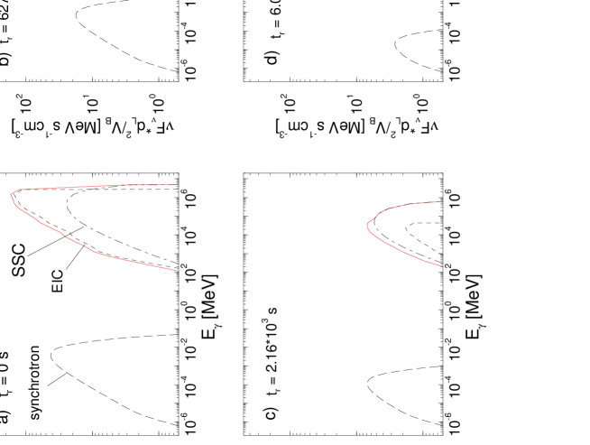
Figure 9: Instantaneous $\gamma$-ray spectra from the blob of simulation 2. Parameters: $\gamma_{1}=6\cdot 10^{3}$, $\gamma_{2}=5\cdot 10^{5}$, $s=2.0$, $R_{B}=8\cdot 10^{15}$ cm, $n=0.2$ cm^-3, $B_{0}=0.07$, $B\propto z^{-0.1}$, $L_{\rm disk}=10^{43}\,{\rm erg\,s}^{-1}$, $M_{BH}=10^{6}\,M_{\odot}$, $z_{i}=10^{-2}$ pc, $\Gamma=20$, $\theta=2^{0}$. Total emission: solid; IC scattering of accretion disk radiation: dashed; SSC radiation: dot-dashed; synchrotron radiation: long dashed. (all quantities in the observer’s frame)

If a second mechanism contributes to the cooling of the radiating pair population, the resulting external inverse-Compton photon spectra do not significantly differ from the case of a pure EIC model. Equally the assumption of a lower cutoff does not have an important effect on the high-energy $\gamma$-ray spectrum. The hard X-ray to soft $\gamma$-ray spectrum from EIC becomes harder with increasing lower cutoff, implying that in case of a high lower cutoff this part of the photon spectrum is always dominated by SSC.

Time-averaged SSC-dominated $\gamma$-ray emission can not account for strong spectral breaks $\Delta\alpha\lower 4.0pt\hbox{$\buildrel>\over{\sim}$}0.5$ in the MeV range as observed in several FSRQs, even if a high lower cut-off in the particle in the initial particle distributions is assumed. This fact is well illustrated by Figs. 8 and 10. In contrast, such a cut-off can produce sharp spectral breaks ($\Delta\alpha>0.5$) in the time-averaged EIC spectrum.

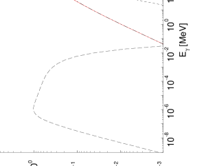
Figure 10: Time-integrated $\gamma$-ray spectrum from the blob illustrated in Fig. 9 (total $\gamma$-ray spectrum: solid; external IC: dashed; SSC: dot-dashed; synchrotron: long dashed)

We find that even in the case of an accretion disk of very low luminosity and injection of the pairs occurring relatively high above the disk EIC scattering will give a significant contribution to the photon spectrum in the GeV – TeV range (see Fig. 10). If our assumption of a two-component $\gamma$-ray spectrum with neither SSC nor EIC being negligible is correct, we conclude that the intrinsic GeV – TeV spectrum of blazars will in general not be a simple power-law extrapolation of the EGRET spectrum.

The particle density plays a central role for the broadband emission from ultrarelativistic plasma blobs. The $\gamma$-ray spectra of blazars can well be reproduced by dense blobs ($n\gg 10^{4}\,{\rm cm}^{-3}$). But in this case, escape of high-energy $\gamma$-rays without significant $\gamma$-$\gamma$ absorption implies the presence of a very low magnetic field and a very weak synchrotron component. This problem is very severe for high-frequency peaked BL Lacs (as Mrk 421) where the $\gamma$-ray component can extend up to TeV energies at which they can be absorbed very efficiently by the synchrotron component if one assumes that both components are produced in the same volume.

In the case of very high density ($n\lower 4.0pt\hbox{$\buildrel>\over{\sim}$}10^{7}$ cm^-3) the cut-off to lower frequencies in the synchrotron spectra is not caused by synchrotron-self absorption but by the Razin-Tsytovich effect. The same effect would also suppress synchrotron cooling below the Razin-Tsytovich frequency (Eq. [25]) which could consequently lead to a storage of the kinetic energy in pairs as long as the magnetic field does not change dramatically and the jet remains well collimated. As mentioned above, this effect can only be important if the synchrotron component (also above the Razin-Tsytovich frequency) is very low compared to the $\gamma$-ray component during a $\gamma$-ray outburst.

Then, a time lag between a $\gamma$-ray flare and the associated radio outburst can give information about the geometry of the jet structure. We suggest that this fact could be a major reason for the difference between FR I and FR II radio galaxies: If the jet is well-collimated over kpc scales, the Razin-Tsytovich effect prevents efficient cooling of the relativistic pairs to Lorentz factors lower than the Razin Lorentz factor, and the kinetic energy of the jet material can only be released in the radio lobes of FR II galaxies. If collimation is inefficient and the jet widens up rapidly after injection, its kinetic energy can be dissipated at short distances from the central engine, which would result in an FR I structure.

8 Model fits to Mrk 421

We can now use our code and the results summarized in the last section to reproduce the broadband spectrum of the first extragalactic object significantly detected in TeV $\gamma$-rays, Mrk 421. Mrk 421 is a BL Lac object at $z=0.031$ which exhibited a prominent TeV flare in May 1994 (Kerrick et al., 1995). In this flaring phase, a flux of $(2.1\pm 0.3)\cdot 10^{-10}$ photons cm^-2 s^-1 above 250 GeV has been found. We assume $H_{0}=75\,{\rm km\,(s\cdot Mpc)}^{-1}$, account for absorption by the intergalactic infrared background radiation (IIBR) using the model fits by (Stecker & de Jager 1996) which do not differ very much from each other for photons of energies $\lower 4.0pt\hbox{$\buildrel<\over{\sim}$}1$ TeV and neglect absorption by accretion disk radiation scattered back by surrounding clouds (Böttcher & Dermer 1995).

Our first example, shown in Figs. 7 and 8, demonstrates that jet parameters are possible where the $\gamma$-ray emission from Mrk 421 in its quiescent state can emerge from a small region where light-travel time arguments allow for even more rapid flickering in $\gamma$-rays than observed recently by Gaidos et al. (1996). As illustrated in Fig. 11, the synchrotron emission from this emission region is far below the observed radio to optical flux from Mrk 421.

Figure 11: Comparison of the time-averaged photon flux from simulation 1 (Figs. 7, 8) to the broadband spectrum of Mrk 421 in its quiescent state, indicated by squares (data from Macomb et al. [1996])

A successful fit to the broadband spectrum of Mrk 421 in its quiescent state can be achieved with a very low density, as chosen for our second example, illustrated in Figs. 9 and 10. This is shown in Fig. 12.

Figure 12: Comparison of the time-averaged photon flux from simulation 2 (Figs. 9, 10) to the broadband spectrum of Mrk 421 in its quiescent state

The flaring state of Mrk 421 can result from an increase of the maximum Lorentz factors of the pairs which could be related to some increase of energy input in hydromagnetic turbulences accelerating the primary particles which can plausibly also imply an increase in the magnetic field. Increasing the cut-off energies to $\gamma_{1}=8\cdot 10^{3}$, $\gamma_{2}=7\cdot 10^{5}$ and the magnetic field to $B=0.08$ G while the other parameters remain the same is in our model calculation for the low state (see caption of Fig. 9) yields an acceptable fit to the flaring state of Mrk 421, as shown in Fig. 13. Here, we integrated over an observing time of $\sim 2\cdot 10^{3}$ s, after which the the flux from this blob is far below the quiescent one.

Figure 13: Model fit to the broadband spectrum of Mrk 421 in its high state (stars); $\gamma_{1}=8\cdot 10^{3}$, $\gamma_{2}=5\cdot 10^{5}$, $B_{0}=0.08$ G; other parameters as given in the caption of Fig. 9

Petry et al. (1996) found a spectral index of the differential spectrum of Mrk 421 above 1 TeV of $3.6\pm 1.0$ which translates to a spectral index of the integral spectrum of $2.6\pm 1.0$. In Figure 14 we demonstrate that our model fit to the low state of Mrk 421 is in agreement with this measurement. Above 1 TeV, absorption by the IIBR becomes important. In order to account for this, we used the model fits by Stecker & de Jager (1996). The figure demonstrates that both fits result in very similar absorbed spectra. The HEGRA flux value is obtained in averaging over long observing times compared to the variability of Mrk 421. It lies between the Whipple data points for quiescent and flaring state (included in Figs. 11 – 13) and is well in agreement with a duty cycle of 5 % between high and low TeV state (Petry, priv. comm.).

Figure 14: Integral photon flux resulting from simulation 2. The dotted and dot-dashed lines represent a power-law integral spectrum with spectral index 2.6 and 3.6, respectively. The solid and dashed lines are calculated describing absorption by the intergalactic infrared background radiation by Stecker & de Jager’s (1996) model fit 1 and 2, respectively

It is remarkable that the broadband fits shown here imply an injection height of $z_{i}\approx 10^{-2}$ pc which is far outside the $\gamma$-ray photosphere for TeV photons. A high low-energy cutoff in the electron spectrum is required in order not to overproduce the X-ray flux. This, in turn, implies a very low particle density in order to recover the observed relative luminosity of the synchrotron to the SSC component.

9 Summary and conclusions

We gave a detailed discussion of the various radiative energy loss mechanisms acting in relativistic pair plasmas and concentrated on the application to jets from active galactic nuclei. In the first phase after the acceleration or injection of pairs radiative cooling due to inverse-Compton scattering is the dominant process. Here, Klein-Nishina effects are much more pronounced for inverse-Compton scattering of external radiation (from the central accretion disk) than for the SSC process since the synchrotron spectrum extends over a much broader energy distribution, allowing for efficient Thomson scattering at all particle energies.

We developed a computer code which allows to follow the evolution of the energy distributions of electrons/positrons self-consistently, accounting for all Klein-Nishina effects and for the time-dependence of the synchrotron, SSC and external radiation fields which contribute to the radiative cooling of the pairs and computing the instantaneous $\gamma$-ray production from the resulting pair distributions. Since the intrinsic cooling timescales are much shorter than the time resultion of present-day instruments, we calculated time-integrated spectra and compared them to observations.

We found some general results from a series of different simulations:

(a) Due to the short cooling times involved in the SSC radiation mechanism, implying that we only see time-integrated SSC emission leading to an overprediction of hard X-ray flux from blazars, we favor EIC to be the dominant radiation process in $\gamma$-ray blazars.

(b) Detailed simulations show that the EIC spectrum of a cooling ultrarelativistic pair distribution with maximum energies implying EIC scattering in the Klein-Nishina regime is harder in the case of pure Thomson scattering where we recover the classical results of Dermer & Schlickeiser (1993 a).

(c) The low-energy cutoff in the synchrotron spectra from dense pair jets is not determined by synchrotron self-absorption, but by the Razin-Tsytovich effect. Only when the jet widens up, radio emission at $\nu\lower 4.0pt\hbox{$\buildrel<\over{\sim}$}10^{11}$ Hz can escape the jet.