The Dynamical Inverse Problem for
Axisymmetric Stellar Systems

Abstract

The standard method of modelling axisymmetric stellar systems begins from the assumption that mass follows light. The gravitational potential is then derived from the luminosity distribution, and the unique two-integral distribution function $f(E,L_{z}^{2})$ that generates the stellar density in this potential is found. It is shown that the gravitational potential can instead be generated directly from the velocity data in a two-integral galaxy, thus allowing one to drop the assumption that mass follows light. The two-dimensional rotational velocity field can also be recovered in a model-independent way. Regularized algorithms for carrying out the inversions are presented and tested by application to pseudo-data from a family of oblate models.

Rutgers Astrophysics Preprint Series No. 190

1 INTRODUCTION

Modelling of elliptical galaxies has a long history, extending back to a time when it was taken for granted that elliptical galaxies were axisymmetric and that all of their mass could be accounted for in stars. We now know that dark matter is a commmon component of galaxies, both at large (Ashman 1992) and small (Kormendy & Richstone 1995) radii, and that triaxial configurations are possible ones for stellar systems (Schwarzschild 1979).

One goal of modern dynamical studies is accordingly to verify the presence of dark matter; another is to detect departures from axisymmetry. Because triaxial models are difficult to construct, one often begins by looking for simpler models that are consistent with the data. This “model-building” approach is popular since it requires a minimum of thought about the information content of the data: one simply builds a model and checks whether it reproduces the observations. But one can take a more sophisticated approach, and ask whether the data imply anything definite about the observed stellar system. For instance, one might attempt to falsify the axisymmetric hypothesis in a model-independent way. This “inverse problem” approach is more difficult but also more rewarding, since it leads to more secure conclusions about the dynamical state of the galaxy.

Beginning with Binney, Davies & Illingworth’s (1990) pioneering study, a standard scheme has been developed for modelling elliptical galaxies. One assumes that the observed galaxy is axisymmetric and that the distribution of mass is known – for instance, mass might be assumed to follow light. The gravitational potential is then derived from this mass distribution using Poisson’s equation; the unique two-integral distribution function $f(E,L_{z})$ that reproduces the stellar density in this potential (or more exactly, the even part of $f$) can also be found (Lynden-Bell 1962; Hunter 1975). The odd part of $f$, which determines the rotational velocity field, is usually represented via some ad hoc parametrization. One then projects this derived $f$ back into observable space to find the predicted kinematical variables and compares them with the observations. If there is agreement, one can claim to have found an axisymmetric model that is consistent with the data.

This technique has been used to reproduce the kinematical data for a few, well-observed elliptical galaxies (van der Marel et al. 1994; Dehnen 1995; Qian et al. 1995). But it is difficult to state precisely what has been learned from studies like these. Are the observed galaxies actually characterized by a constant $M/L$, axisymmetry, and a two-integral distribution function, as assumed? Or might there exist models with spatially-varying $M/L$’s or three-integral $f$’s that reproduce the data equally well? And if no model consistent with the data can be found, which of the various assumptions made in the model-building has been violated?

A useful comparison can be made here with spherical systems (§2.1). If one assumes that the gravitational potential $\Phi(r)$ of a spherical galaxy is known, then the observed velocity dispersion profile can be used to infer the unique dependence of anisotropy on radius (Binney & Mamon 1982). Alternatively, one can assume that the distribution of stellar velocities is everywhere isotropic, in which case the velocity dispersion profile implies a unique form for $\Phi(r)$ (Merritt & Gebhardt 1994). Assuming both isotropy and a constant $M/L$ would clearly be an over-determination of the problem, since the two assumptions together imply a unique velocity dispersion profile, and this predicted profile would almost certainly be different from the observed profile – indeed, the kinematical data would not have been used at all in the construction of the model. But this is precisely what is commonly done in modelling axisymmetric galaxies: one assumes both isotropy in the meridional plane (i.e. $f=f(E,L_{z})$) as well as an ad hoc form for the potential, and these two assumptions together imply a unique dependence of the mean square velocity on position over the image of the galaxy. It is unlikely that a model constructed in this way would reproduce the two-dimensional velocity dispersion data; and if it did not, there would be no clear indication of which assumption had been violated.

It is clearly desirable to think more carefully about the information content of kinematical data in axisymmetric stellar systems. Unlike the spherical case, the functions to be derived depend on two spatial variables, but the kinematical data are likewise two-dimensional, depending on both projected radius and position angle. Many such data sets now exist, for stars in globular clusters (Meylan et al. 1995) and in galaxies (Bacon et al. 1994); emission-line objects around the Galactic bulge (te Linkel Hekkert et al. 1991) and around other galaxies (Hui et al. 1995); and galaxies in clusters (Colless & Dunn 1996). These data are most often in the form of discrete velocities, and in the best-studied systems, the measured velocities number in the hundreds or even thousands.

Here it is shown (§2.2) that the availability of two-dimensional kinematical data allows one to approach the dynamical study of axisymmetric stellar systems as an inverse problem rather than as a model-building problem. From the single Ansatz $f=f(E,L_{z})$, one can infer the unique gravitational potential $\Phi(\varpi,z)$ that is consistent with the observed first and second velocity moments of $f$. The rotational velocity field can likewise be obtained in a model-independent way. By using the kinematical data in the construction of the model, rather than assuming that mass follows light, one thus arrives at the unique pair of functions $\{f,\Phi\}$ that are consistent with the two-integral hypothesis. If this unique model can be falsified – for instance, by using line-of-sight velocity distributions, proper motions, or some other data – then the two-integral, axisymmetric hypothesis will have been convincingly ruled out. In the model-building approach, on the other hand, one can not discard the two-integral assumption until one has explored an effectively infinite number of possible forms for the potential (§2.3).

The numerical techniques that are required for converting the velocity data into a map of the potential are rather more subtle than the ones that have been applied up to now in the study of axisymmetric galaxies. These techniques are accordingly described in some detail (§3.1) before applying them to pseudo-data generated from a family of oblate models (§3.2, 3.3).

Although this approach yields the unique potential consistent with the two-integral assumption for $f$, the true potential might be different if $f$ depends on a third integral. However it would be premature to investigate three-integral models until one had first used the algorithms described here, or equivalent ones, to rule out a two-integral model. Having done so, one could then search for the pair of functions $\{\Phi(\varpi,z)$, $f(E,L_{z},I_{3})\}$ that are most consistent with the data. This is a hard problem, and even in the spherical geometry there is no published algorithm that can extract $\Phi(r)$ and $f(E,L^{2})$ in a completely model-independent way from the data; the most sophisticated such algorithms are still based on parametrized forms for the potential (Saha & Merritt 1993; Merritt 1993b).

The focus here is on situations where the velocities are measured discretely, as would be the case for stars in a globular cluster. Most large, kinematical data sets are of this form.

It is also assumed throughout that the observer lies in the equatorial plane of the observed system. The reason for this unpleasant assumption is that deprojection of the luminosity density becomes underdetermined if the inclination angle is less than $\pi/2$, even if this angle is assumed known (Rybicki 1986; Gerhard & Binney 1996). One can therefore probably not hope to uniquely infer the dynamical state of an axisymmetric galaxy that is not viewed edge-on. This fact is routinely ignored in the model-building studies but must be faced squarely if one wishes to solve the inverse problem.

Also presented here (§3.4) is the first regularized algorithm capable of deriving $f(E,L_{z})$ for an axisymmetric system from its density and potential (the Lynden-Bell – Hunter problem) given imperfect or incomplete information about those functions.

2 THE INVERSE PROBLEM

2.1 Spherical Systems

Our starting point for the axisymmetric inverse problem is the simpler spherical problem. A spherical stellar system has a distribution function that depends on the orbital energy $E$ and angular momentum ${\bf L}$ (both defined here per unit mass). Spherical symmetry in velocity space is assumed as well; then $f=f(r,v)=f(E)=f[v^{2}/2+\Phi(r)]$, and the radial and azimuthal velocity dispersions are everywhere equal, $\sigma_{r}(r)=\sigma_{t}(r)\equiv\sigma(r)$.

Having measured a set of discrete positions and velocities, one can compute smooth approximations to the surface density profile $\Sigma(R)$ and the line-of-sight velocity dispersion profile $\sigma_{p}(R)$. The function $\sigma(r)$ that defines the intrinsic velocity dispersion is then related to the observed velocity dispersions via

$$\Sigma(R)\sigma_{p}^{2}(R)=\int_{R^{2}}^{\infty}\nu(r)\sigma^{2}(r){dr^{2}\over\sqrt{r^{2}-R^{2}}}$$ (1)

which when inverted gives

$$\nu(r)\sigma^{2}(r)=-{1\over\pi}\int_{r}^{\infty}{d(\Sigma\sigma_{p}^{2})\over dR}{dR\over\sqrt{R^{2}-r^{2}}}.$$ (2)

Here $\nu(r)$ is the spatial density of the kinematical sample, obtained by deprojecting the surface density $\Sigma(R)$:

$$\nu(r)=-{1\over\pi}\int_{r}^{\infty}{d\Sigma\over dR}{dR\over\sqrt{R^{2}-r^{2}}}.$$ (3)

The mass within $r$ and the potential follow from Jeans’s equation in spherical symmetry:

$$GM(r)=r^{2}{d\Phi\over dr}=-r\sigma^{2}(r)\left({d\log\nu\over d\log r}+{d\log\sigma^{2}\over d\log r}\right),$$ (4)

and the mass density is

$$\rho(r)={1\over 4\pi r^{2}}{dM\over dr}.$$ (5)

Finally, the unique isotropic distribution function describing the kinematical sample is given by Eddington’s formula:

$$f(E)={1\over\sqrt{8}\pi^{2}}{d\over dE}\int_{E}^{0}{d\nu\over d\Phi}{d\Phi\over\sqrt{\Phi-E}}.$$ (6)

Thus both $f$ and $\Phi$ follow uniquely from the observed surface density and velocity dispersion profiles, under the sole assumption of spherical symmetry in velocity space. Here we are treating the stars as if they were ions in an X-ray emitting gas; the quantity $\sigma^{2}(r)$ plays the role of $kT(r)/m$ in the gas, and no assumption has been made that mass follows light.

In spite of its limitations, this approach has the following things to recommend it.

1. One begins from a statement of the problem that is fully determined: there is a unique pair of functions $\{f(E),\Phi(r)\}$ that reproduce any set of observed profiles $\{\Sigma(R),\sigma_{p}(R)\}$. In practice one does not measure $\Sigma(R)$ or $\sigma_{p}(R)$ precisely, but nonparametric algorithms can be defined which yield estimates $\{\hat{f},\hat{\Phi}\}$ that are suitably close to the true functions (Merritt & Gebhardt 1994).

2. The dependence of $\Phi$ on $r$ is determined from the velocity data, as it should be, rather than being derived from the luminosity density under the always-questionable assumption that mass follows light.

3. The validity of the single assumption – that $f$ is spherically symmetry in velocity space – can be checked. One simply projects the derived model to find the predicted, joint distribution of positions and line-of-sight velocities:

$$N(R,v_{p})=\pi\int_{R^{2}}^{r_{max}^{2}(V)}{dr^{2}\over\sqrt{r^{2}-R^{2}}}\int_{0}^{-2\Phi(r)-v_{p}^{2}}f\left[v^{\prime 2}/2+v_{p}^{2}/2+\Phi(r)\right]dv^{\prime 2}.$$ (7)

If this function is consistent with the observed line-of-sight velocity distribution at every radius, then the model is fully consistent with the data (assuming that no other relevant data exist); if not, isotropy can be ruled out, independent of any preconceptions about the radial variation of M/L.

Often the kinematical data will be insufficient in quality or quantity to produce a statistically significant discrepancy with the computed $N(R,v_{p})$, because anisotropy generates only slight changes in the form of the line profiles and very high quality data are required to detect these changes (Gerhard 1993; Merritt 1993b). Nevertheless this approach makes manifest a point that is often misunderstood: one can not, in principle, make inferences about the degree of velocity anisotropy in a spherical system from the velocity dispersion data alone, since one can always construct the potential in such a way as to reproduce any observed $\sigma_{p}(R)$.

4. For some stellar systems – e.g. globular clusters – the assumption of isotropy in velocity space can be physically motivated.

2.2 Axisymmetric Systems

Our goal is to identify a similar inverse problem for axisymmetric stellar systems. We wish to show that complete knowledge of the line-of-sight velocity moments ${\overline{v}}_{p}$ and $\overline{v_{p}^{2}}$ on the plane of the sky, and of the surface density $\Sigma$ of the kinematical population, is equivalent to knowledge of the two-integral distribution function $f(E,L_{z})$ describing that population and of the potential $\Phi(\varpi,z)$ in which it moves – independent of any assumptions about the relative distribution of mass and light. As discussed above, it is assumed throughout that the observer lies in the equatorial plane of the observed system.

The Jeans equations that relate the potential $\Phi(\varpi,z)$ of an axisymmetric system to gradients in the velocity dispersions are

$$\nu{\partial\Phi\over\partial z} = -{\partial(\nu\sigma_{z}^{2})\over\partial z}-{\partial(\nu\overline{v_{\varpi}v_{z}}\varpi)\over\varpi\partial\varpi},$$ (8)

$$\nu{\partial\Phi\over\partial\varpi} = -{\partial(\nu\sigma_{\varpi}^{2})\over\partial\varpi}-{\partial(\nu\overline{v_{\varpi}v_{z}})\over\partial z}-{\nu\over\varpi}\left(\sigma_{\varpi}^{2}-\overline{v}_{\phi}^{2}-\sigma_{\phi}^{2}\right).$$ (9)

Here $(\varpi,z,\phi)$ are the usual cylindrical coordinates; all quantities are assumed independent of $\phi$.

Now set $f=f(E,L_{z})$. The velocity dispersions are then isotropic in the meridional plane, $\sigma=\sigma_{\varpi}=\sigma_{z}$, and the Jeans equations reduce to

$$\nu{\partial\Phi\over\partial z} = -{\partial(\nu\sigma^{2})\over\partial z},$$ (10)

$$\nu{\partial\Phi\over\partial\varpi} = -{\partial(\nu\sigma^{2})\over\partial\varpi}-{\nu\over\varpi}\left(\sigma^{2}-\overline{v}_{\phi}^{2}-\sigma_{\phi}^{2}\right).$$ (11)

Define Cartesian coordinates $(X,Z)$ on the plane of the sky, with $Z$ parallel to the symmetry axis and $Y$ along the line of sight. We assume that $\nu(\varpi,z)$ has been derived from $\Sigma(X,Z)$ via the usual inversion, unique for an edge-on galaxy (Rybicki 1986). $\Phi(\varpi,z)$ is still unknown. But if we multiply the first Jeans equation by $\partial/\partial\varpi~{}\nu^{-1}$ and the second by $\partial/\partial z~{}\nu^{-1}$ and equate, we find a relation between $\sigma_{\phi}$, $\overline{v}_{\phi}$ and $\sigma$ that is independent of $\Phi$:

$${\partial\nu\over\partial\varpi}{\partial\sigma^{2}\over\partial z}-{\partial\nu\over\partial z}{\partial\sigma^{2}\over\partial\varpi}+{\nu\over\varpi}{\partial\over\partial z}\left(\sigma^{2}-\sigma_{\phi}^{2}-\overline{v}_{\phi}^{2}\right)=0.$$ (12)

This relation may be seen as specifying a unique $\sigma_{\phi}$ given $\sigma$ and $\overline{v}_{\phi}$, i.e.

$$\overline{v}_{\phi}^{2}(\varpi,z)+\sigma_{\phi}^{2}(\varpi,z)=\overline{v^{2}_{\phi}}(\varpi,z)=-\varpi\int_{z}^{\infty}\nu^{-1}(\varpi,z)\left[{\partial\nu\over\partial\varpi}{\partial\sigma^{2}\over\partial z}-{\partial\nu\over\partial z}{\partial\sigma^{2}\over\partial\varpi}\right]dz+\sigma^{2}(\varpi,z).$$ (13)

Now consider the rotational velocity field. The mean line-of-sight velocity $\overline{v}_{p}(X,Z)$ is related to the internal streaming velocity $\overline{v}_{\phi}(\varpi,z)$ via the projection integral

$$\Sigma(X,Z)\overline{v}_{p}(X,Z)=2X\int_{X}^{\infty}\nu(\varpi,Z)\overline{v}_{\phi}(\varpi,Z){d\varpi\over\sqrt{\varpi^{2}-X^{2}}}$$ (14)

(Fillmore 1986, Eq. 12). Equation (14) has inversion

$$\nu(\varpi,z)\overline{v}_{\phi}(\varpi,z)=-\varpi{1\over\pi}\int_{\varpi}^{\infty}{d\over dX}\left[X^{-1}\Sigma(X,z)\overline{v}_{p}(X,z)\right]{dX\over\sqrt{X^{2}-\varpi^{2}}}.$$ (15)

Note that $\overline{v}_{\phi}$ is completely determined by $\overline{v}_{p}$ independent of the two-integral assumption – all that is required here is the assumption of axisymmetry. The possibility of computing the rotational velocity field via direct inversion of the data has been pointed out (though never implemented) by a number of authors including Meylan & Mayor (1986) and Merrifield (1991).

The mean square line-of-sight velocity is

$$\Sigma(X,Z)\overline{v_{p}^{2}}(X,Z)=2\int_{X}^{\infty}\nu(\varpi,Z)\left[\left(1-{X^{2}\over\varpi^{2}}\right)\sigma^{2}(\varpi,Z)+{X^{2}\over\varpi^{2}}\overline{v^{2}_{\phi}}(\varpi,Z)\right]{\varpi d\varpi\over\sqrt{\varpi^{2}-X^{2}}}$$ (16)

(Fillmore 1986, Eq. 16). The integrand on the right hand side contains the two unknown functions $\sigma^{2}$ and $\overline{v^{2}_{\phi}}=\overline{v}^{2}_{\phi}+\sigma^{2}_{\phi}$, and at first sight does not admit of a unique inversion. But we have a relation between $\sigma^{2}$ and $\overline{v^{2}_{\phi}}$, equation (13). We can therefore replace $\overline{v^{2}_{\phi}}$ in the integrand by a linear expression that depends only on $\sigma^{2}$ and on $\nu$. Although no analytic expression for the inverse relation could be found by the author, it will be shown below that $\sigma^{2}(\varpi,z)$ is numerically well-determined by this equation. Having derived $\sigma^{2}(\varpi,z)$, $\overline{v^{2}_{\phi}}(\varpi,z)$ then follows from equation (13), and $\sigma^{2}_{\phi}=\overline{v^{2}_{\phi}}-\overline{v}^{2}_{\phi}$.

It has thus been shown that $\overline{v}_{\phi}(\varpi,z)$, $\sigma_{\phi}(\varpi,z)$ and $\sigma(\varpi,z)$ are determined by the two-dimensional velocity moment data in an edge-on, two-integral system without any assumptions aside from isotropy in the meridional plane. It follows that the potential $\Phi(\varpi,z)$ and the mass density $\rho(\varpi,z)$ are also known: the former from equations (10) or (11), the latter from Poisson’s equation:

$$\rho(\varpi,z)={1\over 4\pi G}\left[{1\over\varpi}{\partial\over\partial\varpi}\left(\varpi{\partial\Phi\over\partial\varpi}\right)+{\partial^{2}\Phi\over\partial z^{2}}\right].$$ (17)

So derived, $\rho$ will of course not necessarily be proportional to $\nu$.

Finally, there is a unique distribution function $f(E,L_{z})$ describing the kinematical population that reproduces $\nu$ and $\overline{v}_{\phi}$ in the derived potential. As usual, we divide $f$ into odd and even parts with respect to $L_{z}$:

$$f(E,L_{z})=f_{+}(E,L_{z})+f_{-}(E,L_{z}),\ \ \ \ f_{\pm}(E,L_{z})\equiv{1\over 2}\left[f(E,L_{z})\pm f(E,-L_{z})\right].$$ (18)

The number density is related to $f_{+}$ via

$$\nu(\varpi,z)={4\pi\over\varpi}\int_{\Phi}^{0}dE\int_{0}^{\varpi\sqrt{2(E-\Phi)}}f_{+}(E,L_{z})dL_{z},$$ (19)

and the rotational velocity field is related to $f_{-}$ via

$$\nu(\varpi,z)\overline{v}_{\phi}(\varpi,z)={4\pi\over\varpi^{2}}\int_{\Phi}^{0}dE\int_{0}^{\varpi\sqrt{2(E-\Phi)}}f_{-}(E,L_{z})L_{z}dL_{z}.$$ (20)

These equations imply unique functions $f_{+}$ and $f_{-}$ given $\nu$, $\overline{v}_{\phi}$ and $\Phi$ (Lynden-Bell 1962; Hunter 1975; Dejonghe 1986), although the inverse relations are complex. Once again, since mass is not assumed proportional to light, the population described by this $f$ will not necessarily have the same spatial distribution as the matter that determines the potential.

Practical algorithms for carrying out the inversions, suitable for real (i.e. noisy and incomplete) data, are described below.

Just as in the spherical case, the validity of the assumed relation between $\sigma_{\varpi}$ and $\sigma_{\phi}$ can be verified by computing the full distribution of line-of-sight velocities $N(X,Z,v_{p})$ from the model and comparing with the observed velocity distributions; or by carrying out the same procedure with the predicted and observed proper motions; etc. If these predicted and observed distributions are significantly different, one can conclude that the assumption of isotropy in the meridional plane is not valid (or that the system is not being viewed edge-on, or is not axisymmetric) and proceed to investigate more general models.

Note that – just as in the spherical case – one can not infer the presence of velocity anisotropy ($\sigma_{z}\neq\sigma_{\varpi}$) based on inspection of the velocity dispersions alone, since the potential can always be constructed so as to reproduce the observed dispersions without a third integral. Information about the dependence of $f$ on a third integral is contained only in the higher-order moments of the line-of-sight velocity distribution (or the proper motions); and conversely, there is no need to use that extra information unless one intends to investigate three-integral models – the two-integral problem is fully constrained by the the first and second velocity moments of $f$.

2.3 Comparison with Other Methods

It is interesting to compare this approach to the one pioneered by Binney, Davies & Illingworth (1990); their technique has recently formed the basis of a number of data-based studies by van der Marel and collaborators (van der Marel, Binney & Davies 1990; van der Marel 1991; van der Marel et al. 1994). Similar approaches to the axisymmetric inverse problem have been worked out by Merrifield (1991), Dejonghe (1993), Emsellem, Monnet & Bacon (1994), Dehnen (1995), Kuijken (1995), and Qian et al. (1995). All of these authors assume at the outset that mass follows light (or that the mass distribution has some other ad hoc form, often including a central point mass), and derive the two-dimensional potential from the assumed mass distribution using Poisson’s equation. The depth of the potential, or equivalently the mass-to-light ratio, is obtained from the virial theorem. The observed velocities are not otherwise used in the construction of the model, except insofar as they constrain the form of the odd part of $f$, which is typically represented via some simple parametrization.

The advantage of this method is its simplicity: once the potential is specified, the even part of the distribution function $f_{+}(E,L_{z})$ or any of its moments can be obtained (Lynden-Bell 1962; Hunter 1975; Dejonghe 1986). But this simplicity is achieved at the cost of having to assume the forms of $\Phi(\varpi,z)$ and $f_{-}$ at the outset. It was shown above that the potential follows uniquely from the observed $\overline{v}_{p}(X,Z)$ and $\overline{v_{p}^{2}}(X,Z)$ in a two-integral, edge-on system – one is not free to assume arbitrary functional forms for $\Phi$. Furthermore the odd part of $f$ can be derived in a model-independent way from the observed rotational velocity field. It follows that the approach taken by these authors is overdetermined. Models constructed in an assumed potential are unlikely to reproduce a two-dimensional set of velocity dispersions, since the information contained in those data was not used. And if the model should fail to reproduce the kinematical data, the failure could be due to the breakdown of either of two assumptions: that mass follows light, or that $f$ depends on only two integrals. In the method described here, on the other hand, the potential is constructed to have the unique form that is consistent with the two-integral assumption for $f$ and with its lowest observable moments. A failure of the model to reproduce any additional kinematical data could only mean that $f\neq f(E,L_{z})$.

The model-building technique has nevertheless been successfully applied to a few galaxies, notably M32 (van der Marel et al. 1994; Dehnen 1995; Qian et al. 1995). But this apparent success should be interpreted with caution. It is possible that these galaxies satisfy all of the assumptions made in the model building, i.e. axisymmetry, $f=f(E,L_{z})$, and $M/L=$ constant. But it is also possible that the published models would fail to reproduce a full, two-dimensional set of velocities if such data were available. Future observations of these galaxies should reveal which of these two possibilities is correct.

Of course, Binney, Davies & Illingworth (1990) were concerned with situations where the kinematical data are confined to just a few cuts across the image of the galaxy. Given such limited data, their approach seems entirely justified. At the same time, our discussion makes clear that – when two-dimensional data are available, as is increasingly often the case – one can and should infer the kinematics and potential directly from the velocities.

Merrifield (1991) proposed a test for the sufficiency of two-integral models when describing edge-on, axisymmetric galaxies. His test is based on the assumption that mass follows light, and uses as a discriminant the measured velocity dispersions. Since one can always construct the potential so as to reproduce the velocity dispersion data in a two-integral system, as shown here, conclusions based on Merrifield’s test are contingent on the assumption that mass follows light.

3 PRACTICAL INVERSION ALGORITHMS

The formal solutions given above to the axisymmetric inverse problem are of little use when dealing with real data, since the inversion equations are ill-conditioned in the sense understood by statisticians (Miller 1974; O’Sullivan 1986). This means that errors or incompleteness in the data will be amplified when going from data space to model space unless some objective smoothness condition is placed on the solution. The degree to which errors are amplified depends on the number of effective differentiations that separate the model from the data. For instance, the distribution function $f(E,L_{z})$ is essentially a second derivative of the number density (Eq. 19) which is itself a half-order derivative of the surface brightness (Eq. 3) – hence the determination of $f$ is strongly ill-conditioned even though formally unique. Some authors have ignored this element of the problem and carried out direct deprojections without imposing smoothness constraints. The results tend to be spectacularly noisy (e.g. Figure 2 of Kuijken 1995). Another approach, equally ill-advised, is to replace the data by ad hoc fitting functions for which the inversions can be carried out exactly (e.g. Qian et al. 1995). Unless these smooth functions are generated from the data using a nonparametric algorithm, they will contain a bias that is likewise amplified by the inversion. Solutions obtained in this way may look appealing in a $\chi^{2}$ sense but are likely to be far from the true solutions.

Richardson-Lucy iteration (e.g. Dehnen 1995) is genuinely nonparametric, going in discrete steps from an initial guess to the (ill-defined) solution that would have been obtained via direct inversion of the data. However the success of this technique depends on the accuracy of the initial guess. A bad guess will require many iterations before the projected solution approximates the data, at which point the solution is likely to be unacceptably noisy. One typically halts the iteration before this occurs but the solution so obtained will accordingly be biased in the direction of the initial guess by some unknown amount. Furthermore, solutions obtained in this way tend to achieve their optimal degree of smoothness in one part of solution space while remaining undersmoothed in other parts.

Our goal is an algorithm which generates solutions that are characterized by acceptably small values of both the noise and the bias. Modern nonparametric methods (Müller 1980; Härdle 1990; Wahba 1990; Scott 1992; Green & Silverman 1994) are designed with precisely this goal in mind. These methods make no assumptions about the global form of the solutions; they deal with the ill-conditioning by imposing smoothness via an effectively local constraint on the level of fluctuations in the solution, an approach called “regularization.” They thus avoid the pitfalls of both Richardson-Lucy iteration (no regularization) and model fitting (parametric bias).

Our focus is on situations where the velocities are measured discretely, as would be the case for stars in a globular cluster, planetary nebulae around a galaxy, galaxies in a cluster, etc. Modifying the algorithms to deal with spatially-continuous data is straightforward.

We assume that the number density profile $\nu(\varpi,z)$ of the kinematical sample is known. Nonparametric algorithms for estimating $\nu$ in the spherical geometry have been described by Merritt (1993a) in the case that the surface brightness is measured directly, and by Merritt & Tremblay (1994) in the case that the surface brightness must first be inferred from discrete positions. These algorithms are easily generalized to the axisymmetric case. We also continue to assume, as discussed above, that the observer lies in the equatorial plane of the observed system, since otherwise the inverse problem is guaranteed not to have a unique solution (Gerhard & Binney 1996).

3.1 A Variational Problem

The inverse problems to be solved here belong to a class of problems that have been well studied by statisticians in the last few years (e.g. Wahba 1990). Let the data be $d_{1},d_{2},...,d_{n}$ and the model $u$. The data are related to the model via

$$d_{i}={\cal L}_{i}u+e_{i},$$ (21)

where the ${\cal L}_{i}$ are known linear functionals – in our case, projections – of $u$, and the $e_{i}$ represent measurement errors or scatter from some other source. For instance, in the determination of the rotational velocity field $\overline{v}_{\phi}$, we would have

$$u=\overline{v}_{\phi}(\varpi,z)$$ (22)

and

$${\cal L}_{i}u = 2X_{i}\Sigma(X_{i},Z_{i})^{-1}\int_{X_{i}}^{\infty}\nu(\varpi,Z_{i})u(\varpi,Z_{i}){d\varpi\over\sqrt{\varpi^{2}-X_{i}^{2}}}$$ (23)

$$= \overline{v}_{p}(X_{i},Z_{i}),$$

the observed rotation at point $(X_{i},Z_{i})$. If the line-of-sight rotational velocity were measured directly, then $d_{i}=\overline{v}_{p}(X_{i},Z_{i})$ and the $e_{i}$ would be measurement errors. If instead discrete velocities were measured, then $d_{i}=v_{i}$, the observed velocity of the $i$th star, and $e_{i}=v_{i}-\overline{v}_{p}(X_{i},Z_{i})$, the deviation (due both to measurement errors and to the intrinsic velocity dispersion) of the $i$th star’s measured velocity from the true mean line-of-sight velocity at point $(X_{i},Z_{i})$.

We seek a smooth function $\hat{u}$ such that ${\cal L}\hat{u}$ is suitably close to the data. One possible approach is to construct a continuous approximation to the function represented by the data – e.g. $\overline{v}_{p}(X,Z)$ – using a kernel or spline smoother, and then to operate mathematically on this function via the inverse operator ${\cal L}^{-1}$ (if it exists) to produce the estimate $\hat{u}$. This approach is consistent in the sense defined by statisticians as long as the functions that are fit to the data are asymptotically unbiased, i.e. nonparametric (Wahba 1990, p. 19), and such an approach has been used with success by Merritt & Gebhardt (1994) to solve the dynamical inverse problem in spherical geometry. Such an approach will not be followed here because one of the inverse problems that we wish to solve – the recovery of $f(E,L_{z})$ from $\nu$, $\overline{v}_{\phi}$ and $\Phi$ – does not have a simple inverse operator. In addition, one sometimes wishes to place physical constraints (e.g. positivity) on the solutions and this is extremely difficult to do if the function approximations are carried out in data space rather than solution space.

Instead we define our solutions implicitly, as the functions $\hat{u}$ that minimize functionals of the form

$$n^{-1}\sum_{i=1}^{n}\left({\cal L}_{i}u-d_{i}\right)^{2}+\lambda J(u).$$ (24)

The first term in equation (24) measures the fidelity of the model to the data. Minimizing this term alone would lead to an unacceptably noisy solution due to the ill-conditioning of the inverse operator. The second term measures the degree to which the solution is unsmooth. One standard choice for the “penalty function” $J(u)$ is

$$J(u)=J_{m}(u)=\sum_{\alpha+\beta=m}{m!\over\alpha!\beta!}\int\int\left({\partial^{m}u\over\partial x^{\alpha}\partial y^{\beta}}\right)^{2}dxdy,\ \ \ \ m\geq 2.$$ (25)

(Here and below, a two-dimensional $u=u(x,y)$ is assumed.) The function $\hat{u}$ that minimizes equation (24) with penalty function (25) is the so-called “thin plate spline” solution (Duchon 1977; Meinguet 1979). Remarkably, this solution can be found in essentially analytic form for many simple operators ${\cal L}$ (Wahba & Wendelberger 1980).

The qualitative nature of the solution to equations (24) and (25) depends on the choices of $\lambda$ and $m$. The penalty function acts as a low-pass filter, with $\lambda$ controlling the half-power point of the filter and $m$ the steepness of the roll-off (Craven & Wahba 1979). Typically one chooses $m=2$; the smoothness of the solution is then controlled by varying $\lambda$. Too large a value for $\lambda$ will oversmooth the solution, i.e. reduce its curvature; too small a value will yield an overly noisy solution. The larger the data set and the smaller the measurement errors, the smaller the value of $\lambda$ that can be profitably used and the more accurate the solution. Thus the bias – the average deviation of the solution from the true function – falls to zero as the sample size $n$ is increased. In parametric algorithms, by contrast, the bias remains finite even as $n$ tends to infinity, since the adopted parametric form is guaranteed to be incorrect at some level and this incorrectness does not diminish as $n$ is increased. It is for this reason that parametric methods are unsuited to data-based inverse problems.

Data are typically incomplete or cover only a limited region. The use of a penalty function guarantees that the solution will tend toward a predictable form in parts of solution space that are not strongly constrained by the data. For instance, the thin-plate spline solution with $m=2$ yields a solution that is linear in $x$ and $y$ wherever the data do not force a different functional form, since any linear function is assigned zero penalty by expression (25). This very useful feature of solutions found via penalty functions means that there is never any need to extend or augment the data in ad hoc ways. Nonparametric techniques based on direct smoothing of the data, e.g. via kernels, do not share this nice property.

Many variations on this basic scheme exist. If the data errors are not normally distributed, one can choose the first term in equation (24) to be some more robust measure of the fidelity of the model to the data. Such a modification would be appropriate in the study of galaxy cluster dynamics where interlopers are common. Another variation is to modify the form of the penalty function. The simplest such variation is to add a factor $k^{m-\alpha}$ with $k$ some positive constant; changing $k$ is equivalent to changing the units in which $y$ is measured. One can also include in the penalty function a weighting function $w(x,y)$ that is large where the solution $u$ is expected to be small, thus encouraging the fluctuations in the solution to remain a fixed fraction of $u$ in amplitude everywhere. Finally, one can replace the differential operator $\partial^{m}\over\partial x^{\alpha}\partial y^{\beta}$ by some more complicated operator, which defines as “perfectly smooth” some different class of functions (e.g. Silverman 1982).

For many choices of $J(u)$, including the thin plate penalty function defined above, the quantity to be minimized is quadratic in $u$. This means that a standard quadratic programming routine (Rustagi 1994) can be used to find the solution on some grid in model space. The use of a quadratic programming algorithm also allows the easy imposition of linear constraints, such as positivity, on the solution if desired.

There is a huge literature concerning the choice of the smoothing parameter $\lambda$. While “objective” schemes exist, a standard practice is to slowly decrease $\lambda$ until the solution begins to exhibit small-scale fluctuations, then stop.

3.2 The Rotational Velocity Field

Consider first the recovery of the rotational velocity field in the meridional plane $\overline{v}_{\phi}(\varpi,z)$. We seek the function $\hat{\overline{v}}_{\phi}$ that minimizes

$$\chi^{2}=\sum_{i=1}^{n}\left({v}_{i}-{\cal L}_{i}{\overline{v}_{\phi}}\right)^{2}+\lambda\int\int\left[\left({\partial^{2}{\overline{v}}_{\phi}\over\partial\varpi^{2}}\right)^{2}+2\left({\partial^{2}{\overline{v}}_{\phi}\over\partial\varpi\partial z}\right)^{2}+\left({\partial^{2}{\overline{v}}_{\phi}\over\partial z^{2}}\right)^{2}\right]d\varpi dz,$$ (26)

with $v_{i}$ the measured velocities and

$${\cal L}_{i}{\overline{v}_{\phi}}=2X_{i}\Sigma(X_{i},Z_{i})^{-1}\int_{X_{i}}^{\infty}\nu(\varpi,Z_{i}){\overline{v}}_{\phi}(\varpi,Z_{i}){d\varpi\over\sqrt{\varpi^{2}-X_{i}^{2}}}.$$ (27)

We choose $\overline{v}_{\phi}$ as our function to be optimized rather than the physically more natural choice $\nu\overline{v}_{\phi}$, since $\overline{v}_{\phi}$ is expected to be a more nearly linear function of the coordinates and hence better suited to a second-derivative penalty function.

We begin by defining a Cartesian grid in model space, $\varpi_{j}=\varpi_{1}+(j-1)\delta\varpi$, $1\leq j\leq N$, and $z_{k}=z_{1}+(k-1)\delta z$, $1\leq k\leq N$. The variables to be solved for are the $N^{2}$ values $v_{j,k}$ of the rotational velocity on the grid. The derivatives and integrals on the right hand side of (26) can easily be represented as linear combinations of the $v_{j,k}$ using standard expressions from numerical analysis; for details from a very similar problem, see Merritt & Tremblay (1994). Placing the $v_{j,k}$ into a linear vector ${\bf g}$, one can then write

$$\chi^{2}={\bf g}^{T}{\bf A}{\bf g}-{\bf B}{\bf g}+C$$ (28)

where the quantities ${\bf A}$, ${\bf B}$ and $C$ are straightforward to compute but messy and will not be given here. The resulting expression is quadratic in the unknowns, and the constraints $v_{j,k}\geq 0$ are linear. The values ${\hat{v}}_{j,k}$ that minimize $\chi^{2}$ can accordingly be found via quadratic programming.

Figure 1 shows an estimate of ${\overline{v}_{\phi}}(\varpi,z)$ derived using 5000 discrete velocities drawn randomly from an oblate model belonging to Lynden-Bell’s (1962) family. The adopted model is the flattest one consistent with non-negative $f$, having $b/a=0.638$ in Lynden-Bell’s notation and $a=-0.814$ in the notation of Dejonghe (1986). (These models have non-constant ellipticity, becoming spherical at large radii for all values of $b/a$.) The odd part of $f$, which specifies the degree of ordered motion, was set to the function derived in the appendix of Lynden-Bell’s paper when generating the Monte-Carlo data. The resultant rotational velocity field has $\sigma_{\varpi}=\sigma_{\phi}=\sigma_{z}$ everywhere, an “oblate isotropic rotator.” Note that even this extreme model from Lynden-Bell’s sequence is only mildly flattened, except very near the center, and the rotation is correspondingly small; the peak rotation velocity is only about one half of the central, one-dimensional velocity dispersion. In spite of the small signal, however, the inversion algorithm recovers the rotational velocity field reasonably well near the center; the main defect is a too-shallow rise of the rotation velocity near $\varpi=0$, an inevitable result of the smoothing. This example suggests that data sets consisting of a few thousand velocities are none too large for recovering the rotational velocity field of an axisymmetric system in a model-independent way.

3.3 The Velocity Dispersions and Potential

We now wish to make estimates of $\sigma(\varpi,z)$ and $\sigma_{\phi}(\varpi,z)$. We search for the functions $\hat{\sigma}^{2}$ and $\hat{\overline{v^{2}_{\phi}}}$ that minimize

$$\chi^{2} = \sum_{i=1}^{n}\left[{v}_{i}^{2}-{\cal L}_{i}\left\{\sigma^{2},\overline{v^{2}_{\phi}}\right\}\right]^{2}$$ (29)

$$+ \lambda\int\int\left[\left({\partial^{2}\sigma^{2}\over\partial\varpi^{2}}\right)^{2}+2\left({\partial^{2}\sigma^{2}\over\partial\varpi\partial z}\right)^{2}+\left({\partial^{2}\sigma^{2}\over\partial z^{2}}\right)^{2}\right]d\varpi dz$$

$$+ \lambda\int\int\left[\left({\partial^{2}\overline{v^{2}_{\phi}}\over\partial\varpi^{2}}\right)^{2}+2\left({\partial^{2}\overline{v^{2}_{\phi}}\over\partial\varpi\partial z}\right)^{2}+\left({\partial^{2}\overline{v^{2}_{\phi}}\over\partial z^{2}}\right)^{2}\right]d\varpi dz$$

subject to the constraints of equation (12):

$${\partial\nu\over\partial\varpi}{\partial\sigma^{2}\over\partial z}-{\partial\nu\over\partial z}{\partial\sigma^{2}\over\partial\varpi}+{\nu\over\varpi}{\partial\over\partial z}\left(\sigma^{2}-\overline{v^{2}_{\phi}}\right)=0$$ (30)

as well as the usual positivity constraints. The operator ${\cal L}_{i}$ is now defined as

$${\cal L}_{i}\left\{\sigma^{2},\overline{v^{2}_{\phi}}\right\}=2\Sigma(X_{i},Z_{i})^{-1}\int_{X_{i}}^{\infty}\nu(\varpi,Z_{i})\left[\left(1-{X_{i}^{2}\over\varpi^{2}}\right)\sigma^{2}(\varpi,Z_{i})+{X_{i}^{2}\over\varpi^{2}}\overline{v^{2}_{\phi}}(\varpi,Z_{i})\right]{d\varpi\over\sqrt{\varpi^{2}-X_{i}^{2}}}.$$ (31)

If the velocities contain measurement errors, these should be subtracted in quadrature from the $v_{i}$.

We define a double grid in $\{\varpi,z\}$, with the first $N^{2}$ points containing the $\sigma^{2}$ values and the second $N^{2}$ points the $\overline{v^{2}_{\phi}}$ values. The constraints (30) are approximated via finite-difference derivatives, which have the effect of linking together the values on the two grids. Finally, one obtains $\sigma_{\phi}$ via $\sigma_{\phi}^{2}=\overline{v^{2}_{\phi}}-\overline{v}^{2}_{\phi}$, with $\overline{v}^{2}_{\phi}$ having been recovered in the previous step.

Before applying the algorithm to pseudo-data, one would like some assurance that the information contained in the observed mean-square velocity field $\overline{v_{p}^{2}}(X,Z)$ is sufficient, in principle, to uniquely constrain both $\sigma(\varpi,z)$ and $\sigma_{\phi}(\varpi,z)$. Ideally this hypothesis would be demonstrated by finding analytical expressions for the inverse relations. Such expressions could not be found (which may simply reflect limitations in the author’s mathematical abilities), and instead the case will here be made numerically.

Figure 2 shows how the integrated square error in the solutions $\hat{\sigma}^{2}(\varpi,z)$, $\hat{\sigma}^{2}_{\phi}(\varpi,z)$,

$${\rm ISE}=\int\int\left(\sigma^{2}-\hat{\sigma}^{2}\right)^{2}d\varpi dz+\int\int\left(\sigma^{2}_{\phi}-\hat{\sigma}^{2}_{\phi}\right)^{2}d\varpi dz,$$ (32)

depends on the degree to which the constraints (30) are imposed. That is, these constraints were replaced by

$$-\Delta\leq{\partial\nu\over\partial\varpi}{\partial\sigma^{2}\over\partial z}-{\partial\nu\over\partial z}{\partial\sigma^{2}\over\partial\varpi}+{\nu\over\varpi}{\partial\over\partial z}\left(\sigma^{2}-\overline{v^{2}_{\phi}}\right)\leq\Delta,$$ (33)

with the parameter $\Delta>0$ – a constant at all points on the solution grid – determining how stringently the contraints are imposed. The algorithm was given as input the exact values, on a grid, of the mean square velocity $\overline{v_{p}^{2}}(X,Z)$ of the rotating oblate model of Figure 1. Solutions were then obtained as a function of $\Delta$. Figure 2 demonstrates that the error in the solutions tends to zero along with $\Delta$, which suggests – at least for this particular model – that the constraints (30) contain just enough information to yield the correct inversion. This experiment was repeated for a number of other models from the Lynden-Bell sequence of models. For each model examined, the solution with $\Delta=0$ was found to be extremely close to the true solution. These experiments hardly constitute a rigorous proof that the inversion is uniquely defined for every possible two-integral oblate model, however.

Figures 3a and 3b illustrate the recovery of $\sigma(\varpi,z)$ and $\sigma_{\phi}(\varpi,z)$ given the same 5000 velocities drawn from the rotating oblate model of Figure 1. Given the uniqueness, just demonstrated, of the inversion for this model, the discrepancies apparent in the numerical solutions of Figure 3 are primarily due to the finiteness of the data set rather than to any limitations of the algorithm. Different, 5000-velocity Monte-Carlo realizations of the same model were found to yield solutions that were different in their details but that had roughly the same average error.

The gravitational potential is obtained by applying either of equations (10) or (11), in finite-difference form, to the derived $\sigma$ and $\sigma_{\phi}$. The result is shown in Figures 3c and 3d. The derived potential is remarkably similar to the correct one except for slightly reduced gradients, again an unavoidable result of the smoothing.

3.4 The Distribution Function

We now want to find the functions $f_{+}(E,L_{z})$ and $f_{-}(E,L_{z})$ that generate the estimated number density $\hat{\nu}(\varpi,z)$ and rotational velocity field $\hat{\overline{v}}_{\phi}(\varpi,z)$ in the reconstructed potential $\hat{\Phi}(\varpi,z)$. This is a simpler version of a problem solved in Merritt (1993b), and we follow a similar approach here. A rectangular grid is defined in $(E,L_{z})$-space, and the unknowns ${f_{+}}_{j,k}$ and ${f_{-}}_{j,k}$ are assumed constant over each cell (Figure 4). The configuration-space density at any point $(\varpi,z)$ is the sum of the contributions $\nu_{cell}=4\pi\varpi^{-1}\Delta E\Delta L_{z}{f_{+}}_{j,k}$, for each cell such that ${L_{z}}_{j,k}<\varpi\sqrt{2\left[E-\Phi(\varpi,z)\right]}$. (Cells that lie partly below and partly above this curve contribute by an amount proportional to the area that lies below the curve.) Similarly, each cell contributes $\nu{\overline{v}_{\phi}}_{cell}=4\pi\varpi^{-2}\Delta E\Delta L_{z}^{2}{f_{-}}_{j,k}$ to the estimate of $\nu(\varpi,z)\overline{v}_{\phi}$. The quantity to be minimized is

$$\chi^{2} = \sum_{i=1}^{n}\left({\nu}_{i}-\sum_{cell}\nu_{cell}\right)^{2}+$$ (34)

$$\int\int\left[\lambda_{1}(E)\left({\partial^{2}f_{+}\over\partial E^{2}}\right)^{2}+2\sqrt{\lambda_{1}(E)\lambda_{2}(E)}\left({\partial^{2}f_{+}\over\partial E\partial L_{z}}\right)^{2}+\lambda_{2}(E)\left({\partial^{2}f_{+}\over\partial L_{z}^{2}}\right)^{2}\right]dEdL_{z},$$

in the case of $f_{+}$, and

$$\chi^{2} = \sum_{i=1}^{n}\left({\nu}_{i}{\overline{v}_{\phi}}_{i}-\sum_{cell}\nu{\overline{v}_{\phi}}_{cell}\right)^{2}+$$ (35)

$$\int\int\left[\lambda_{1}(E)\left({\partial^{2}f_{-}\over\partial E^{2}}\right)^{2}+2\sqrt{\lambda_{1}(E)\lambda_{2}(E)}\left({\partial^{2}f_{-}\over\partial E\partial L_{z}}\right)^{2}+\lambda_{2}(E)\left({\partial^{2}f_{-}\over\partial L_{z}^{2}}\right)^{2}\right]dEdL_{z},$$

in the case of $f_{-}$. The integrals are understood to extend over the region in the $(E,L_{z})$ plane such that $0<L_{z}<L_{max}(E)$, where $L_{max}(E)$ is the maximum value of $L_{z}$ attainable at energy $E$ (Fig. 4). The smoothing parameters $\lambda_{1}$ and $\lambda_{2}$ are allowed to depend on the energy since $f$ falls off much more rapidly than linearly with $E$, and a penalty function with constant $\lambda$ would not strongly penalize a solution that was smooth at large $|E|$ but noisy for $E\approx 0$. Furthermore, a different degree of smoothing is permitted in the $E$ and $L_{z}$ directions since $f$ is expected to be much more homogeneous in $L_{z}$ than in $E$.

Figure 5 illustrates the recovery of $f_{+}$ and $f_{-}$ using the approximations to $\Phi(\varpi,z)$ and $\overline{v}_{\phi}$ obtained in the previous sections. The smoothing parameters were chosen to vary as $|E|^{-1.5}$, with $\lambda_{2}/\lambda_{1}=100$. Once again, the only obvious systematic error takes the form of a bias due to the smoothing.

The derivation of $f(E,L_{z})$ given $\nu(\varpi,z)$ and $\Phi(\varpi,z)$ is a classical problem in stellar dynamics. Lynden-Bell (1962), Hunter (1975) and Dejonghe (1986) demonstrated the uniqueness of the solution, and recently Hunter & Qian (1993) have presented an elegant algorithm for carrying out the inversion given analytic expressions for $\nu$ and $\Phi$.

Hunter & Qian’s algorithm is not regularized and hence not suitable for use with real data. It has nevertheless been applied in this way, after first replacing the data with analytic models (Qian et al. 1995). This approach is dangerous at best since any slight error in the choice of fitting functions will be amplified enormously by the inversion operator. Solutions so obtained for $f$ may be smooth and physically appealing, but they are unlikely to be close to the true solutions.

From a numerical point of view, the only non-trivial aspect of solving the Lynden-Bell–Hunter problem is the regularization; the inversion itself is essentially just a matrix operation once the integral operator has been represented via some discrete approximation. Much effort has been directed recently toward refining the discretization (Kuijken 1995) or the inversion (Hunter & Qian 1993), with curiously little attention paid to the more crucial question of regularization.

4 SUMMARY

Given measurements of the line-of-sight rotational velocity and the velocity dispersion over the two-dimensional image of an edge-on, axisymmetric galaxy, one can derive the unique functions $\Phi(\varpi,z)$ and $f(E,L_{z})$ that reproduce those data, without the necessity of assuming that mass follows light. The validity of such a model can then be tested using other data, such as the full line-of-sight velocity distributions or the proper motions. Failure to reproduce the data using this method would imply that $f$ depends on a third integral of motion (or that one of the geometric assumptions, axisymmetry or zero inclination, was violated). This approach is a generalization of the one pioneered by Binney, Davies and Illingworth (1990) which assumes that mass follows light and which derives both $\Phi$ and $f$ from the luminosity distribution alone, without using the kinematical data except in the normalization of $\Phi$. We have presented numerical algorithms, suitable for use with noisy and incomplete data, for carrying out the required inversions and shown that they provide smooth and accurate estimates of $f$ and $\Phi$ using simulated data sets derived from oblate models.

In a companion paper, the algorithms described here will be applied to velocity data from the globular cluster $\omega$ Centauri.

The results described here suggest the following avenues for future work.

1. A mathematical – as opposed to numerical – demonstration of uniqueness (or non-uniqueness) of the solutions to the coupled equations (12) and (16) would be of fundamental importance.

2. The second-derivative penalty functions adopted here are almost certainly non-optimal and it would be worthwhile to investigate more general forms. In addition, it is possible that the solutions to the roughness-penalized inverse problems defined here can be found analytically, as in Wahba & Wendelberger (1980).

3. As shown most recently by Gerhard & Binney (1996), the axisymmetric inverse problem becomes under-determined when the stellar system is viewed from a direction that is not parallel to the symmetry plane. Additional information must therefore be added if one is to solve the inverse problem for an arbitrary orientation. (One would also like to infer that orientation from the data.) There is at present no clear understanding of what form that extra information should take.

4. One can define an alternate inverse problem based on the Ansatz that mass follows light, or more generally that the form of the potential $\Phi(\varpi,z)$ is known a priori; for instance, the potential might be derived from X-ray data, from the statistics of gravitational lensing, etc. This is of course the usual assumption that is made when modelling axisymmetric galaxies; however the goal would be to learn something unique about the degree of velocity anisotropy $\sigma_{\varpi}/\sigma_{z}$ from the velocity moment data, as in the analogous spherical problem (Binney & Mamon 1982). Unfortunately one can show that the assumption of a known potential is not sufficient in itself to uniquely constrain the anisotropy, even for an edge-on system; one must make additional assumptions, e.g. that the velocity ellipsoid is everywhere aligned with the coordinate axes. Nevertheless, more work along these lines would help to elucidate the more difficult inverse problem for a three-integral $f$.

This work was supported by NSF grant AST 90-16515 and NASA grant NAG 5-2803. T. Fridman kindly assisted in the plotting of the figures. I thank W. Dehnen and O. Gerhard for lively discussions on the topic of axisymmetric modelling, and for pointing out some mathematical errors in an early version of the paper. I also thank H. Dejonghe for many useful insights on problems of this sort.

Recovery of the rotational velocity field $\overline{v}_{\phi}(\varpi,z)$ given 5000 velocities derived from an oblate, Lynden-Bell (1962) model with maximum flattening. Heavy contours: estimated $\overline{v}_{\phi}$; thin contours: exact $\overline{v}_{\phi}$.

Dependence of the ISE of the velocity dispersion solutions, Eq. (32), on the parameter $\Delta$ that determines how stringently the constraints (33) are applied.

Recovery of the velocity dispersions and potential from the same data used Fig. 1. Heavy contours: estimated values; thin contours: exact values. (a) $\sigma$; (b) $\sigma_{\phi}$; (c) $\Phi$; (d) $\Phi(\varpi,0)$.

Grid-based scheme for recovery of $f_{+}(E,L_{z})$. (a) Solution grid. Upper curve is the maximum $L_{z}$ as a function of $E$; lower curve is the characteristic curve for a given $(\varpi,z)$. (b) Projection of a single $(E,L_{z})$ grid cell into $(\varpi,z)$-space.

Recovery of $f_{+}(E,L_{z})$ (a) and $f_{-}(E,L_{z})$ (b) given data generated from the oblate Lynden-Bell model. Heavy contours: estimated values; thin contours: exact values.

Figure 1:

Figure 2:

Figure 3:

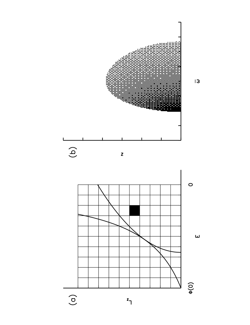
Figure 4:

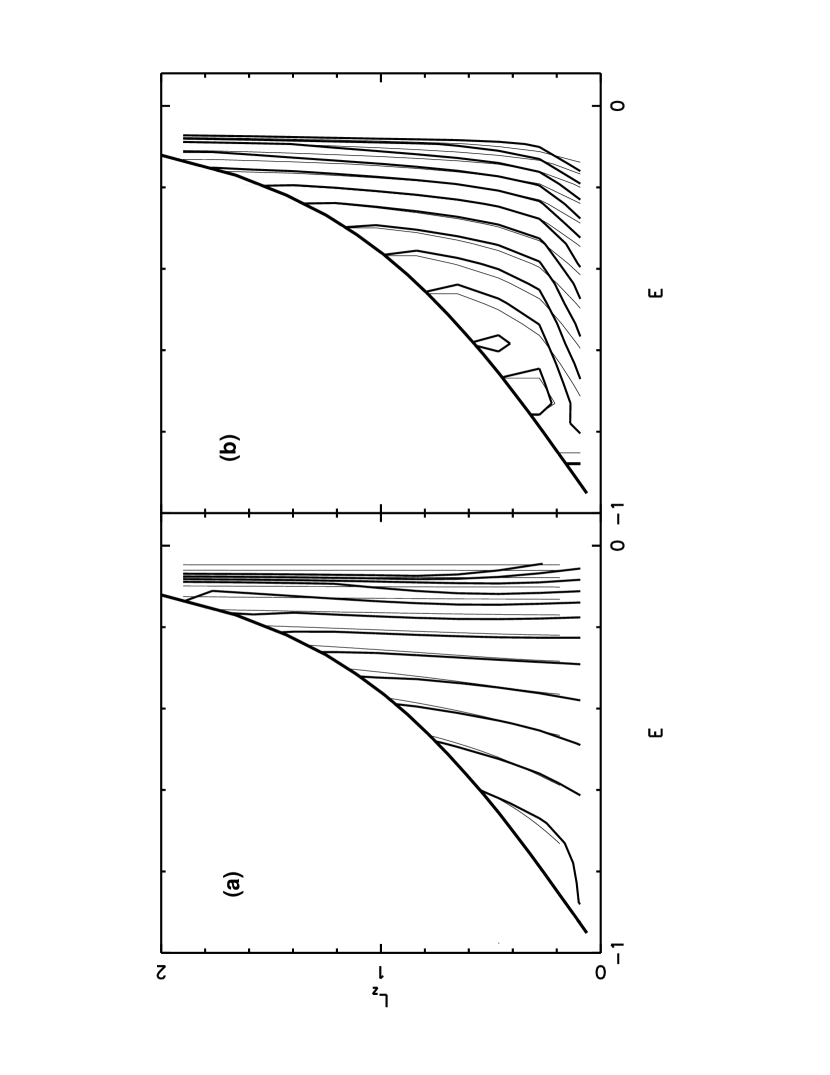
Figure 5:

References

- (1)
- (2)
- (3) Ashman, K. 1992, PASP, 104, 1109
- (4) Bacon, R., Emsellem, E., Monnet, G. & Nieto, J. L. 1994, AAp 281, 691
- (5) Binney, J., Davies, R. & Illingworth, G. 1990, ApJ, 361, 78
- (6) Binney, J. & Mamon, G. A. 1982, MNRAS, 200, 361
- (7) Colless, M. & Dunn, A. M. 1996, ApJ, 458, 435
- (8) Craven, P. & Wahba, G. 1979, Numer. Math. 31, 377
- (9) Dehnen, W. 1995, MNRAS, 274, 919
- (10) Dejonghe, H. 1986, Phys. Rept. 133, 217
- (11) Dejonghe, H. 1993, in Galactic Bulges, IAU Symp. No. 153, ed. H. Dejonghe & H. J. Habing (Kluwer: Dordrecht), 73
- (12) de Zeeuw, P. T. 1985, MNRAS, 216, 273
- (13) Duchon, J. 1977, in Constructive Theory of Functions of Several Variables (Springer: Berlin), 85
- (14) Emsellem, E., Monnet, G., & Bacon, R. 1994, AAp, 285, 723
- (15) Fillmore, J. A. 1986, AJ, 91, 1096
- (16) Gerhard, O. 1993, MNRAS, 265, 213
- (17) Gerhard, O. & Binney, J. 1996, preprint
- (18) Green, P. J. & Silverman, B. W. 1994, Nonparametric Regression and Generalized Models (Chapman & Hall: London)
- (19) Härdle, W. 1990, Applied Nonparametric Regression (Cambridge University Press: Cambridge)
- (20) Hui, X., Ford, H., Freeman, K. C. & Dopita, M. 1995, ApJ 449, 592
- (21) Hunter, C. 1975, AJ, 80, 783
- (22) Hunter, C. & Qian, E. 1993, MNRAS, 262, 401
- (23) Kormendy, J. & Richstone, D. 1995, Ann. Rev. Astron. Astrophys., 33, 581
- (24) Kuijken, K. 1995, ApJ, 446, 194
- (25) Kuzmin, G. G. & Kutuzov, S. A. 1962, Bull. Abastumani Ap. Obs. 27, 82
- (26) Lynden-Bell, D. 1962, MNRAS, 123, 447
- (27) Meinguet, J. 1979, J. Appl. Math. Phys. 30, 292
- (28) Merrifield, M. R. 1991, AJ, 102, 1335
- (29) Merritt, D. 1993a, in Structure, Dynamics and Chemical Evolution of Elliptical Galaxies, ed. I. J. Danziger, W. W. Zeilinger & K. Kjär (ESO: Garching), 275
- (30) Merritt, D. 1993b, ApJ, 413, 79
- (31) Merritt, D. & Gebhardt, K. 1994, in Clusters of Galaxies, Proceedings of the XXIXth Rencontre de Moriond, ed. F. Durret, A. Mazure & J. Tran Thanh Van (Editions Frontiere: Singapore), p. 11.
- (32) Merritt, D. & Saha, P. 1993, ApJ, 409, 75
- (33) Merritt, D. & Tremblay, B. 1994, AJ, 108, 514
- (34) Meylan, G. & Mayor, M. 1986, AA 166, 122
- (35) Meylan, G., Mayor, M., Duquennoy, A. & Dubath, P. 1995, AA 303, 761
- (36) Miller, G. F. 1974, in Numerical Solution of Integral Equations, ed. L. M. Delves & J. Walsh (Clarendon Press: Oxford), 175.
- (37) Müller, H.-G. 1980, Nonparametric Regression of Longitudinal Data (Springer: Berlin)
- (38) O’Sullivan, F. 1986, Stat. Sci. 1, 502
- (39) Qian, E. E., de Zeeuw, P. T., van der Marel, R. P. & Hunter, C. 1995, MNRAS, 274, 602
- (40) Rustagi, J. S. 1994, Optimization Techniques in Statistics (Academic Press: Boston)
- (41) Rybicki, G. B. 1986, in Structure and Dynamics of Elliptical Galaxies, IUA Symp. 127, ed. P. T. de Zeeuw (Kluwer: Dordrecht), 397
- (42) Scott, D. W. 1992, Multivariate Density Estimation, New York: John Wiley & Sons
- (43) Schwarzschild, M. 1979, ApJ, 232, 236
- (44) Silverman, B. 1982, Ann. Stat., 10, 795
- (45) te Linkel Hekkert, P., Caswell, J. L., Habing, H. J., Haynes, R. F. & Norris, R. P. 1991, AAp Suppl. 90, 327
- (46) van der Marel, R. P. 1991, MNRAS, 253, 710
- (47) van der Marel, R. P., Binney, J. & Davies, R. 1990, MNRAS, 245, 582
- (48) van der Marel, R. P., Evans, N. W., Rix, H.-W., White, S. D. M. & de Zeeuw, T. 1994, MNRAS, 271, 99
- (49) Wahba, G. 1990, Spline Models for Observational Data (SIAM: Philadelphia)
- (50) Wahba, G. & Wendelberger, J. 1980, Monthly Weather Review, 108, 1122
- (51)