The Redshift Distribution and Luminosity Functions
of Galaxies in the Hubble Deep Field

Abstract

Photometric redshifts have been determined for the galaxies in the Hubble Deep Field. The resulting redshift distribution shows two peaks: one at $z\sim 0.6$ and one at $z\sim 2.2$. Luminosity functions derived from the redshifts show strong luminosity evolution as a function of redshift. This evolution is consistent with the Babul & Rees (1992) scenario wherein massive galaxies form stars at high redshift while star formation in dwarf galaxies is delayed until after $z=1$.

1 Introduction

The Hubble Deep Field (HDF) optical images are the deepest yet obtained. Objects as faint as $I_{ST}$=28.5 can be detected at the $10\sigma$ level. At this point in time, only a few spectroscopic redshifts have been measured for the brighter galaxies and none for the faintest galaxies in these images.

Photometric redshifts (see, for example, Gwyn 1995; Connolly et al. 1995; Koo 1985) can be measured much faster and to much fainter magnitudes than their spectroscopic counterparts. Because the wavelength bin-size in photometry is generally so much larger than in conventional spectroscopy ($\sim$1000Å  vs. 1–2Å), far shorter exposure times are required to measure redshifts (but with a sacrifice in accuracy).

Photometric redshifts have been calculated for the galaxies brighter than $I_{ST}=28$ in the Hubble Deep Field. This paper presents the redshift distribution for this sample. Also presented are luminosity functions as a function of redshift out to $z=5$.

2 The photometric redshift technique

The photometric redshift technique can be divided into three steps: First, the photometric data for each galaxy in the fields are converted into spectral energy distributions (SED’s). Second, a set of template spectra of all Hubble types and redshifts ranging from $z=0$ to $z=5$ is compiled. Third, the spectral energy distribution derived from the observed magnitudes of each object is compared to each template spectrum in turn. The best matching spectrum, and hence the redshift, is determined by minimizing $\chi^{2}$. In the following subsections, each of these steps is examined.

2.1 Photometry to spectral energy distributions

The magnitude in each bandpass is converted to a flux (power per unit bandwidth per unit aperture area) at the central or effective wavelength, $\lambda_{cen}$, of the bandpass. When the flux is plotted against wavelength for each of the bandpasses, a low resolution spectral energy distribution is created.

The following equation converts magnitudes in some filter, $f$, to fluxes:

$$F_{f}=F_{0}10^{-m_{f}/2.5},$$ (1)

where $m_{f}$ is the apparent magnitude, $F_{f}$ is the flux in units of W Å^-1 m^-2 and $F_{0}$ is the flux zero-point of that filter system in the same units. This equation is simple to use as long as the flux zero-point is known. Unlike almost all other magnitude systems (e.g. the Johnson/Cousins UBVRI system) the flux zero-points for the ST magnitude system are the same for all filters, making the conversion of magnitudes to fluxes straightforward.

2.2 The template spectra

The template spectra were produced from the models of Bruzual & Charlot (1993). They showed that their models faithfully reproduce the spectra of local galaxies. More recently, Steidel et al. (1996a) found that high redshift galaxies are also well described by the models.

The templates were produced in a two-dimensional grid with galaxy type (ranging from Sm to E/S0) in one dimension and redshift (ranging from $z=0$ to $z=5$) in the other. The galaxy templates included evolution according to the Bruzual & Charlot (1993) models. It was assumed that they formed 0.5 Gyr after the Big Bang and evolved reaching an age of 15 Gyr at the present epoch. A cosmology where $H_{0}=50$ km sec^-1 Mpc^-1, $\Omega_{0}=0.3$, and $\lambda_{0}=0$ was used to convert redshift to the evolutionary epoch of the models and in the later calculation of the luminosity functions.

To represent the different galaxy types an interpolation was made between the instantaneous burst model (for early-type galaxies) and the constant star formation rate model (for late-type galaxies). These interpolated spectra were then redshifted. The redshifted spectra were reduced to the passband averaged fluxes at the central wavelengths of the passbands, in order to compare the template spectra with the SED’s of the observed galaxies.

2.3 Comparing the templates to the SED’s

Given a spectral energy distribution of a galaxy of unknown redshift and a set of templates, the next step is to compare the SED to each of the templates in turn and to the template which most closely matches the SED. The degree to which each template matches the observed SED is quantified in the following manner:

$$\chi^{2}=\sum_{i=1}^{N_{f}}{(F_{i}-\alpha T_{i})^{2}\over\Delta F_{i}^{2}},$$ (2)

where $N_{f}$ is the number of filters in the set, $F_{i}$ and $\Delta F_{i}$ are respectively the flux and the uncertainty in the flux in each bandpass of the observed galaxy, $T_{i}$ is the flux in each bandpass of the template being considered, and $\alpha$ is a normalization factor. A normalization factor is necessary to compare properly the galaxies and the templates because the fluxes of the galaxies are very small relative to the fluxes of the templates. Each template is then compared to the target galaxy SED and the smallest value of $\chi^{2}$ is found. The best matching template gives $z_{phot}$, the sought-after photometric redshift of the galaxy.

2.4 Accuracy

The photometric redshift technique has been tested with simulations and photometric observations of galaxies with known spectroscopic redshifts.

2.4.1 Effects of photometric errors

The simulations take the following form: A spectral energy distribution is chosen at random from the template SED’s available. The SED is reduced to fluxes at the central wavelength of the passbands of the filter set to be tested. To simulate observational errors, a small random number with a Gaussian distribution is added to the fluxes in each band of the chosen template. Photometric redshifts are determined from the resulting simulated photometry in the manner described above. These photometric redshifts are compared with the redshifts of the templates from which they were derived.

Not surprisingly, when the errors in the photometry are zero, the photometric redshift technique always picks the correct redshift. As the errors in the photometry increase, so do the errors in the photometric redshifts in the form of the standard deviation of redshift residuals. The simulations indicate that the uncertainties in the photometric redshifts, $\sigma_{pz}$, increase with redshift. For $z<1.5$ they are only $\sigma_{pz}\simeq 0.07$; for $1.5<z<5$ they are $\sigma_{pz}\simeq 0.20$.

2.4.2 Effects of variations in evolutionary history

As a check on the sensitivity of the derived redshifts to a particular evolutionary model, photometric redshifts were calculated for the HDF galaxies using non-evolving templates, i.e. templates derived by redshifting the SED’s of local galaxies. Although in general these photometric redshifts were different from those derived from the evolving templates, no systematic difference was found. These differences can be attributed to the different evolutionary histories of the individual galaxies. The differences represent uncertainties in the redshifts of between $\sigma_{pz}\simeq 0.05$ (low redshift) and $\sigma_{pz}\simeq 0.2$ (high redshift). The lack of a systematic difference can be understood if a portion of the evolution in the SED’s takes the form of a change in galaxy spectral type. Further, the photometric redshift technique is sensitive to the location of large breaks (at 4000Å  and 912Å) which change with redshift, not type or evolutionary state.

2.4.3 Effects of internal absorption by dust

The reddening effects of dust are not accounted for in the Bruzual & Charlot (1993) models. In order to evaluate the effects of dust on the derived redshifts, moderate amounts of internal reddening were added to the template SED’s. Random differences of $\sigma_{pz}\simeq 0.05$ (independent of redshift) were found between the redshift derived from these templates and those derived from un-reddened templates, but again no systematic differences were evident.

2.4.4 Comparison with available spectroscopic redshifts

Some spectroscopic redshifts are available for the HDF: those of Cowie (1996) (23 galaxies with $z<1.5$ at this point in time) and Steidel et al. (1996b) (5 galaxies with $z>1.5$). A comparison of these spectroscopic redshifts and photometric redshifts shows that the uncertainties in the photometric redshifts at high redshift ($z>1.5$) are $\sigma_{pz}\simeq 0.5$. At low redshift, two out of 23 galaxies have redshift discrepancies greater than $\Delta z=0.5$ while the remaining 21 have a standard deviation of $\sigma_{pz}\simeq 0.2$.

When one adds the above uncertainties due to photometry, evolution and moderate internal reddening one finds that $\sigma_{cal}\simeq 0.1$ ($z<1.5$) and $\sigma_{cal}\simeq 0.3$ ($z>1.5$). The observed uncertainties are clearly much larger: $\sigma_{obs}\simeq 0.2$ ($z<1.5$) and $\sigma_{obs}\simeq 0.5$ ($z>1.5$). However, it is not difficult to imagine additional sources of uncertainty. Among them are absorption by the intervening IGM (both gas and dust) and evolutionary metal abundance effects. Both of these effects are difficult to quantify and given the primarily statistical nature of this investigation we rely on the empirically derived uncertainties.

3 The redshift distribution and luminosity function

The positions of the galaxies in the HDF images were taken from the catalogs of Couch (1996). Magnitudes were measured for all galaxies from the HDF Version 2 images through a 0.2 arc-second radius aperture using IRAF. The photometric redshift technique was used on all galaxies brighter than $I_{ST}>28$. A small fraction (6%) of the galaxies have no $U_{ST}$ magnitudes; redshift for these galaxies were calculated using only the $B_{ST}R_{ST}I_{ST}$ photometry. These redshifts are somewhat less accurate but have the same distribution as the 4-colour redshifts. Three galaxies have no measurable $U_{ST}$ or $B_{ST}$ flux. Photometric redshifts cannot be calculated for them; they were ignored in the following discussion.

The redshift distribution is shown in Figure 1. The distribution shows two peaks, one at a redshift of about $z\simeq 0.6$ and another at $z\simeq 2.2$. The redshift distribution of the of the galaxies without $U_{ST}$ magnitudes is shown as a dashed line. Compared to spectroscopic redshifts, where typically $\Delta z\sim 0.001$, the uncertainties associated with photometric redshifts are large. Note, however, that the width of the bins in this histogram (0.4 in $z$) are comparable to the errors expected in the photometric redshifts ($\sigma_{pz}\sim 0.2-0.5$). Simulations indicate that this level of precision is sufficient to calculate accurate luminosity functions. Indeed, photometric redshifts have been used at $z\sim 0.35$ to calculate LF’s identical to those determined using spectroscopic redshifts (Gwyn 1995).

The luminosity functions (LF’s) were constructed using the $1/V_{a}$ method. The $1/V_{a}$ method is well known and has been described in detail elsewhere (Schmidt 1968; Lilly et al. 1995b) so the following description is brief.

$V_{a}$ is defined as the volume accessible to a galaxy given its absolute magnitude and the limits defining the sample in which it is found. Formally,

$$V_{a}=\int_{z_{min}}^{z_{max}}{dV\over dz}dz,$$ (3)

where $dV/dz$ is the co-moving differential volume element. The limits, $z_{min}$ and $z_{max}$ can be fixed (as in a volume limited sample), but for a magnitude limited sample they must be determined for every galaxy. Given the absolute magnitude, $M$, of each galaxy and the limiting apparent magnitude of the sample, $m_{lim}$, the limiting redshift at which the galaxy would still be in the sample, $z_{lim}$, can be determined. The luminosity function, $\Phi$, is the sum of the inverse of the accessible volumes ($\sum 1/V_{a}$) normalized to the angular area surveyed.

The luminosity function was calculated for three redshift regions: $z<1$, $1<z<3$ and $3<z<5$. In each case, $z_{min}$ was the lower bound of each redshift region ($z=$0, 1 and 3 respectively). The minimum of the upper bound of each redshift region ($z=$1, 3 and 5 respectively) or $z_{lim}$ (as determined for each galaxy using $I_{ST}=28.0$ for $m_{lim}$) was used for $z_{max}$.

The luminosity functions thus calculated are shown in Figure 2. In order to compare the luminosity functions with local LF’s, they are shown in the (Johnson) $B$ band. Note that it is not necessary when using the $1/V_{a}$ method to use the same filter to calculate both the $V_{a}$’s and the absolute magnitudes.

Shown for comparison as a solid line is the local luminosity function of Loveday (1992). The lowest redshift division ($z<1$, dotted line) shows the steep faint end of the local luminosity function. The next highest redshift division ($1<z<3$, dashed line) lacks this faint tail; the space density of faint galaxies seems depressed with respect to the $z<1$ LF. The bright end is about 4 magnitudes brighter than the local luminosity function. The bright end is fainter by about 0.5 magnitudes in the highest redshift interval ($3<z<5$, dot-dashed line); the faint end drops off at a brighter magnitude. Although different cosmologies change the positions (and, to a lesser degree, the shape) of the luminosity functions, changing the parameters does not greatly alter the relative positions of the LF’s at various redshifts.

These variations in the luminosity function with redshift can be explained if there are two epochs at which galaxies undergo their first major burst of star formation. The first occurs before $z\mbox{${\scriptstyle\buildrel>\over{\sim}}$}2.2$; at this time the larger galaxies start forming stars. The galaxies do not all burst simultaneously. The stars of some galaxies first turn on at $z\sim 5$, some form as late as $z\sim 2$ while most form at $z\sim 2.2$, corresponding to the peak of the redshift distribution shown in Figure 1. Depending on the fraction of gas that is converted into stars in the initial starburst, a fading of 4 magnitudes since $z\sim 2.2$ is entirely consistent with the Bruzual & Charlot (1993) models.

The heuristic model of Broadhurst, Ellis & Shanks (1988) of starbursting dwarfs at moderate redshifts was put on a more physical basis by Babul & Rees (1992) and Babul & Ferguson (1996) who postulated that star formation in dwarf galaxies is delayed until $z\sim 1$ by photoionization of their gas by inter-galactic ultraviolet radiation. This second epoch of star formation explains the observed excess at moderate redshifts of faint blue galaxies (termed “boojums” for “blue objects observed just undergoing moderate starburst” by Babul & Rees, 1992). These galaxies end up on the steeply rising faint tail of the lowest redshift luminosity function. This scenario would also explain why the higher redshift luminosity functions in Figure 2 have depressed faint ends: the galaxies that would populate the faint end haven’t turned on yet.

4 Summary

Using photometric redshifts, a redshift distribution has been determined for the Hubble Deep Field. It shows two peaks: one at $z\simeq 0.6$ and another at $z\simeq 2.2$. Luminosity functions have been calculated using these redshifts. The LF’s show strong evolution: the brightest galaxies are 4 magnitudes brighter than their present day counterparts and the faint galaxies are fewer in number. The double-peaked redshift distribution and the evolution of the luminosity function can be understood if larger galaxies form stars early at $z\sim 3$ and if star formation is delayed in the dwarf galaxies until after $z\simeq 1$.

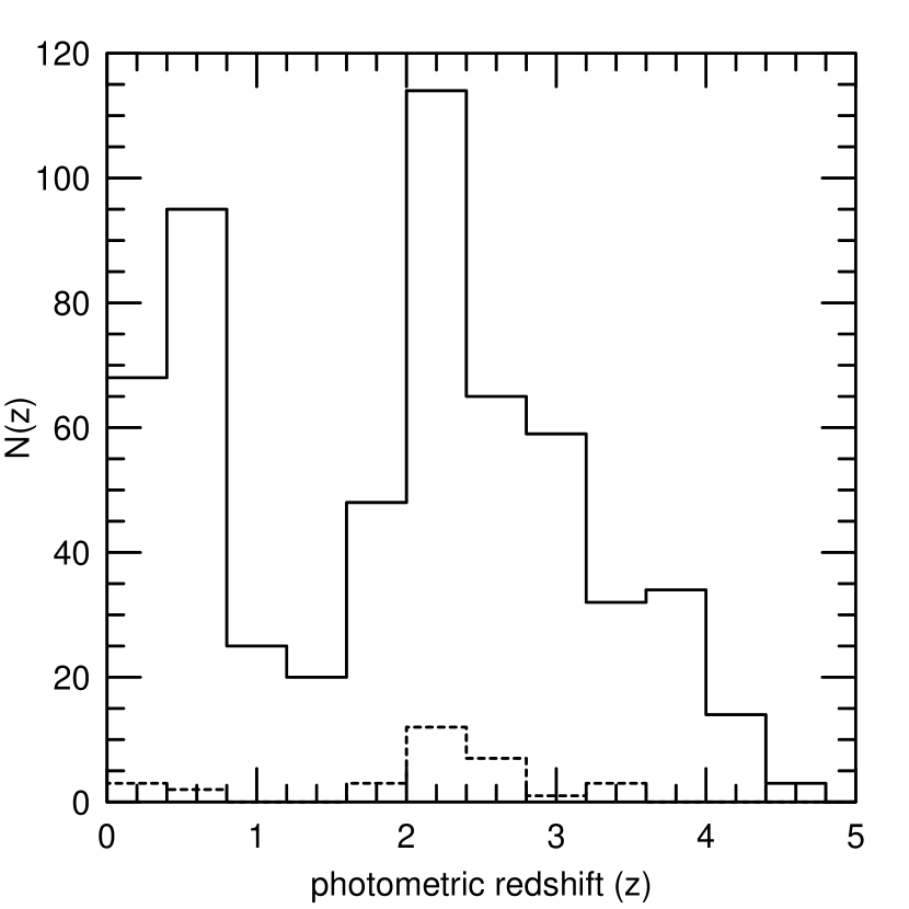
Figure 1: The HDF redshift distribution. Two peaks are visible in the distribution: one at $z\sim 0.6$ and one at $z\sim 2.2$. The redshift distribution of those galaxies for which $U_{ST}$ is not available is shown as a dashed line.

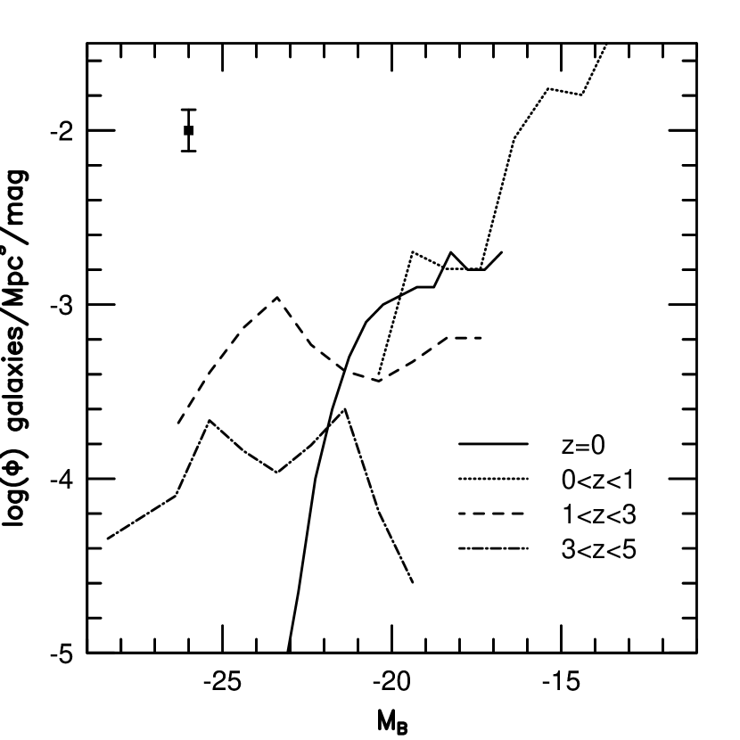
Figure 2: The evolution of the (Johnson) $B$ luminosity function with redshift. The local LF is that of Loveday et al. (1992). The error bar shows the typical $1/\sqrt{N}$ $N^{-{1\over 2}}$ uncertainties which represent a lower limit to the true uncertainties.

References

- Babul & Ferguson, (1996) Babul, A. & Ferguson, H. C. 1996, ApJ, 458, 100
- Babul & Rees, (1992) Babul, A. & Rees, M. J. 1992, MNRAS, 255, 364
- (3) Broadhurst, T. J., Ellis, R. S., & Shanks, T. 1988, MNRAS, 235, 827
- (4) Bruzual, G. A. & Charlot, S. 1993, ApJ, 405, 538
- (5) Connolly, A. J., Csabai, I., Szalay, A. S., Koo, D. C., Kron, R. G., & Munn, J. A. 1995, AJ, 110, 2655
- (6) Couch, W. J. 1996, Public communication, [http //ecf.hq.eso.org/hdf/catalogs]
- (7) Cowie, L. L. 1996, Public communication, [http://www.ifa.hawaii.edu/ cowie/hdf.html]
- (8) Gwyn, S. D. J. 1995, unpublished M.Sc. thesis, University of Victoria
- (9) Koo, D. C. 1985, AJ, 90, 418
- (10) Lilly, S. J., Tresse, L., Hammer, F., Crampton, D., & Le Fèvre, O. 1995b, ApJ, 455, 108
- (11) Loveday, J., Peterson, B. A., Efstathiou, G., & Maddox, S. J. 1992, ApJ, 390, 338
- Schmidt, (1968) Schmidt, M. 1968, ApJ, 151, 393
- (13) Steidel, C. C., Giavalisco, M., Pettini, M., Dickinson, M., & Adelberger, K. L. 1996a, Preprint [astro-ph/9602024]
- (14) Steidel, C. C., Giavalisco, M., Dickinson, M., & Adelberger, K. L. 1996b, Preprint [astro-ph/9604140]