The Structure and Dynamical Evolution of Dark Matter Halos

Abstract

We use $N$-body simulations to investigate the structure and dynamical evolution of dark matter halos in clusters of galaxies. Our sample consists of nine massive halos from an Einstein-De Sitter universe with scale free power spectrum and spectral index $n=-1$. Halos are resolved by 20000 particles each, on average, and have a dynamical resolution of 20-25 kpc, as shown by extensive tests. Large scale tidal fields are included up to a scale $L=150$ Mpc using background particles. We find that the halo formation process can be characterized by the alternation of two dynamical configurations: a merging phase and a relaxation phase, defined by their signature on the evolution of the total mass and root mean square (rms) velocity. Halos spend on average one third of their evolution in the merging phase and two thirds in the relaxation phase. Using this definition, we study the density profiles and show how they change during the halo dynamical history. In particular, we find that the average density profiles of our halos are fitted by the Navarro, Frenk & White (1995) analytical model with an rms residual of 17% between the virial radius $R_{v}$ and $0.01R_{v}$. The Hernquist (1990) analytical density profiles fits the same halos with an rms residual of 26%. The trend with mass of the scale radius of these fits is marginally consistent with that found by Cole & Lacey (1996): compared to their results our halos are more centrally concentrated, and the relation between scale radius and halo mass is slightly steeper. We find a moderately large scatter in this relation, due both to dynamical evolution within halos and to fluctuations in the halo population. We analyze the dynamical equilibrium of our halos using the Jeans’ equation, and find that on average they are approximately in equilibrium within their virial radius. Finally, we find that the projected mass profiles of our simulated halos are in very good agreement with the profiles of three rich galaxy clusters derived from strong and weak gravitational lensing observations.

1 Introduction

Observational studies of galaxy clusters are providing ever more data that need theoretical interpretation in order to understand cluster formation and evolution. In current cosmological models the mass and dynamics of galaxy clusters are dominated by some kind of non-baryonic, dark matter, which interacts with ordinary baryonic matter only through gravity. In studies focussing on the dynamics of galaxy clusters, they can thus be regarded as halos made of collisionless dark matter. From the theoretical point of view one can study the structure of dark matter halos both analytically and numerically. Much of the analytical work done so far is based on the secondary infall paradigm, (Gunn & Gott 1972). The simplest version of this picture considers an initial point mass, which acts as a nonlinear seed, surrounded by an homogeneous uniformly expanding universe. Matter around the seed slows down due to its gravitational attraction, and eventually falls back in concentric spherical shells with purely radial motions. Calculations based on this model predict that the density profile of the virialized halo should scale as $\rho(r)\propto r^{-9/4}$. Self similar solutions were found by Fillmore & Goldreich (1984) and by Bertschinger (1985). Hoffman & Shaham (1985) applied an extension of this idea to the gravitational instability theory of hierarchical clustering. In their calculations they assumed a Gaussian random field of initial density perturbation with scale-free power spectra: $P(k)\propto k^{n}$. They found that the virialized structures originating from density peaks should have density profiles whose shape depends on spectral index $n$ as $\rho(r)\propto r^{-(9+3n)/(4+n)}$.

In reality the collapse of an initial overdensity is not so simple. In particular, motions are not purely radial, and accretion does not happen in spherical shells (as assumed in the secondary infall model), but by aggregation of subclumps of matter which have already collapsed; a large fraction of observed galaxy clusters exhibit significant substructure (Kriessler et al. 1995). It is therefore very important to complement and compare these analytical studies with numerical simulations. These are not bound by such restrictions and so can tell if the gravitational collapse of a collisionless system eliminates all memory of the cosmological parameters which determined its initial conditions. They can also show whether scale-free universes, which have no characteristic scale, give rise to scale-free power-law density profiles. Work in this direction includes Quinn, Salmon & Zurek (1986), Efstathiou et al. (1988) and West, Dekel & Oemler (1987), but the somewhat conflicting results of these studies show that better numerical resolution is needed to settle the issue. Recent results from higher resolution simulations (Navarro et al. 1995 (hereafter NFW), Lemson 1995, Cole & Lacey 1996 (hereafter CL), Xu 1996), produced by different $N$-body codes with different setups for the initial conditions, seem finally to agree on the following results:

1. halo density profiles are curved, and are well approximated by a fitting formula governed by a single scale radius $r_{s}$ and belonging to the family of curves: $\rho(r)\propto x^{-\alpha}(1+x^{\beta})^{-\gamma}$, $x=r/r_{s}$. NFW propose a model with $(\alpha,\beta,\gamma)=(1,1,2)$; another candidate is the Hernquist (1990) (hereafter HER) profile: $(\alpha,\beta,\gamma)=(1,1,3)$.

2. These fitting formulae provide a good model for halos formed in simulations of both scale-free and cold dark matter (CDM) universes.

3. The value of the scale radius $r_{s}$ depends both on the initial cosmology and on the mass of the halo in a way apparently related to the formation time of the halos.

Interestingly, a mass dependence for the scale radius was also found observationally by Sanders & Begeman (1994), who used the HER model to fit the dark matter component when modelling the rotation curves of a sample of spiral galaxies.

Despite the recent wealth of studies on this subject, the computational limits of present day machines are such that simulations of galaxy clusters are only now starting to reach a resolution sufficient to resolve reliably the dark matter structure of the central $\sim$ 100 kpc. As a result several issues are still waiting for more detailed study. Among them: have the results presented so far converged? That is, are they independent of numerical limitations? Does the trend of the scale radius with halo mass depend on numerical resolution? Are the simulated halos in dynamical equilibrium? And, especially, do halo dynamics affects halos structure, for example, the shape of density profiles, and the scatter in the relation between the halo mass and the scale radius $r_{s}$?

More generally, the distribution of dark matter in the central regions of the halo is of particular interest; for example, the ability of a cluster to act as a gravitational lens, producing multiple magnified images of background galaxies, depends crucially on the mass content of the very central part (few tens of kpc) of the cluster, hence on the slope of the density profile at that scale. Further questions to ask are then: what is the structure of cluster-size halos in the central few tens of kpc? Are results of simulations compatible with recent lensing observations?

The purpose of the present paper is to address some of these points. Section 2 presents the simulations. Section 3 is dedicated to extensive numerical tests to establish the reliability of our results. In Section 4 the halo formation process is interpreted using a simple description in terms of its mass and rms velocity. Section 5 presents our main results on halo density profiles, their dependence on the dynamical configuration of the system, analytical fits to them, and the dependence of these fits on halo mass. Section 6 discusses related topics, like the dynamical equilibrium of halos, and the comparison of simulations to dark matter observations from lensing studies. Finally Section 7 summarizes the results and presents some conclusions.

2 The simulations

2.1 Initial Conditions

To generate the initial conditions for a cluster simulation, we took a previously evolved cosmological simulation of a large region, a cube of side $L$, and selected a suitable cluster from this region. The initial conditions in the neighborhood of the cluster were then resampled with higher resolution in the following way. All particles in the final cluster within a sphere of mean overdensity $\delta_{0}$, (typically $\delta_{0}=200$), were traced back to the unperturbed initial conditions, and the Lagrangian region $V_{L}$ containing them was enclosed in a cube of size $L^{\prime}<L$; in our case $L^{\prime}=0.25L-0.4L$ was required. We then replaced the original particles in this cube with a larger number of lower mass particles, and perturbed them according to the same density fluctuations from the parent simulation, together with new fluctuations of higher frequency (up to the new Nyquist frequency), with amplitudes given by the theoretical power spectrum $P(k)$. Since $V_{L}$ is irregular in shape, its volume is only a fraction of the volume ${L^{\prime}}^{3}$, typically 10% to 15% of it. To optimize the use of the high resolution particles for the formation of the cluster, we peeled off the high resolution cube and left high resolution particles only in an irregular high resolution region that closely follows the shape of $V_{L}$, and has a volume roughly twice that of $V_{L}$.

The large-scale density and velocity field of the simulation was modeled as follows. All particles in the original simulation falling outside the high resolution region (referred to as background particles) were selected, and their mass and velocity were interpolated onto a spherical grid, using fixed angular resolution $d\theta=d\phi$, and with $dr=rd\theta$ in order to give approximately cubic cells throughout the sphere. This operation reduces the number of background particles to the minimum necessary to preserve the large-scale tidal field of the original simulation. Detailed tests have shown that a choice $d\theta=7.5^{\circ}$, corresponding to $6000$ to $9000$ background particles, allows an accurate sampling of the tidal field. By construction, the mass of the background particles increases with distance from the high resolution region, and their gravitational softening $s$ was increased accordingly: $s\propto M^{1/3}$. The sphere of background particles was always taken as big as the size $L$ of the parent simulation. The relevant parameter here is the ratio between the maximum wavelength included in the simulation and the size $L^{\prime}$ of the proto-cluster. Since in our case $L^{\prime}$ can be as big as $0.4L$, the fluctuations mainly responsable for the initial density peak in the proto-cluster have wavelength $\lambda\approx 2L^{\prime}-3L^{\prime}$ which is already of the order of the original box size $L$. Therefore, taking a sphere smaller than $L$ would exclude important contributions in the initial fluctuations and so would probably change the final result, although we have not investigated along this direction.

The new initial conditions were finally traced back to a higher redshift, such that the three-dimensional rms initial particle displacement in the high resolution region was less than $0.75\bar{d}$, with $\bar{d}$ the mean interparticle separation. This ensures the validity of linear theory even in the more densely sampled regions. By evolving from these conditions, the formation of the selected cluster can be followed with higher resolution than before, with a reasonably low computational cost. An example of this setup, together with the simulation itself, is shown in Figure 2.

Figure 2: Example of a simulation: time goes from left to right and from top to bottom. The first panel shows the initial conditions of the simulation, at $z=25$. The high resolution region in the centre is formed by $\approx 50000$ particles; the sphere of 8700 background particles of varying mass provides accurate sampling of the large scale tidal field. The diameter of the simulation at $z=25$ is 6 Mpc in proper coordinates. In the following panels, only the high resolution particles are shown, at different redshifts. Each panel represents a region of 12 Mpc (proper) on a side. The circle indicates the virial radius $R_{v}$ of the densest clump of matter in the simulation at that time. At $z=0$ there are roughly 24000 particles within $R_{v}$.

2.2 Simulation details

We started from a cosmological simulation of an Einstein-de Sitter universe, with scale free power spectrum $P(k)\propto k^{n}$, $n=-1$, evolved using a Particle-Particle-Particle-Mesh code (Efstathiou et al. 1985) with $100^{3}$ particles in a $256^{3}$ grid with periodic boundary conditions. The simulation box is 150 Mpc on a side, for a dimensionless Hubble parameter $h=0.5$. All distances given in this paper are for $h=0.5$. We selected the nine most massive clusters formed in the simulation (containing typically a few thousand particles each), set up higher resolution initial conditions for all of them, as described in the last Section, and carried out nine high resolution simulations. For the evolution we used a tree-SPH code (Navarro & White 1993), without gas, i.e. as a pure $N$-body code. This code has individual and arbitrary time stepping (Groom & White 1996, in preparation). The normalization for all simulations is such that at the final time the rms matter density fluctuation in spheres of radius $r=8h^{-1}$ Mpc is $\sigma_{8}=0.63$, in agreement with the observed abundance of local clusters (White et al. 1993).

The virial mass of the clusters, enclosing an average overdensity $\delta\rho/\rho=178$, ranges from $M_{v}=5.2\times 10^{14}M_{\hbox{$\odot$}}$ to about $3\times 10^{15}M_{\hbox{$\odot$}}$, while their one dimensional rms velocity within the virial radius ranges from 700 km s^-1 to 1300 km s^-1. The average number of particles within the virial radius of each cluster is $N_{v}\simeq 20000$. The gravitational softening $s$ imposed on small scales follows a cubic spline profile, and is kept fixed in physical coordinates. Its value is $s=20-25$ kpc at the final time, depending on the simulation. The typical maximum number of timesteps per simulation is of order 20000. Forces softened by a cubic spline can be roughly approximated by a Plummer softening $\epsilon\simeq s/1.4$. The force resolution of our simulations is $L/s\simeq 6000$ to $7500$ for the box and of order of $R_{v}/s\simeq 100$ (with $R_{v}$ the virial radius) for single halos. The mass resolution for one halo is, as we said, of order 20000. The typical central density we resolve in the halos with the innermost 50 particles is of order of $10^{6}$ times the mean background density.

We can compare these parameters with those of recent simulations which have addressed the same issue of the structure of dark matter halos in different cosmological models. We will quote results for the most massive halos in each case.

The scale free $n=-1$ simulation run by Crone et al. (1994) have a force resolution $L/1.4\epsilon=730$ on the simulation box, and of about $R_{v}/1.4\epsilon=30$ for each halo. Their mass resolution is of order of 6000 for the same objects.

The standard CDM simulation by Jing et al. (1994) has force resolution of about $3000$ for the box and 30 for massive halos, and a mass resolution of order 1000 particles for a typical massive halo. They used 400 to 800 timesteps to evolve the system to the present time.

The force resolution in the CDM simulations by NFW is $\approx 12000$ for the box, and like ours ($\sim 100$) for single objects. Their mass resolution is 5000 to 10000 particles per halo. Their typical maximum number of timesteps per simulation is between 10000 and 100000.

Finally, the scale free $n=-1$ simulation performed by CL have a force resolution of about 2700 on the box, and of about 40 on their most massive halos. Their mass resolution on these is about 7000 particles, and they evolved the simulation in $\approx 500$ equal timesteps.

This comparison shows that our simulations are the most accurate run so far, and we hope they will serve as a reference point for further studies. They took on average 200 hours of cpu time each, running on fast workstations. For seven out of nine simulations we have 25 outputs, equally spaced in time from $t=t_{i}$ to the present time $t=t_{0}$. For the other two we have fewer outputs. The main physical and numerical parameters of the simulations are summarized in Table 2. Figure 4 shows, for all halos, the projected dark matter density at $z=0$. As we will show in Section 3, we trust the results of our density profiles down to a distance from the cluster centre equal to the gravitational softening radius. This gives us two order of magnitudes of spatial resolution for the clusters here presented.

Table 2: Main numerical and physical parameters of the nine simulated halos. The column content is: halo coding label; redshift of initial conditions; gravitational softening at $z=0$; number of particles within the virial radius; virial mass; virial radius; one dimensional rms velocity within $R_{v}$; ratio of softening and virial radius; number of minimum timesteps taken by the simulation.

Label	$z_{i}$	$s$	$N_{v}$	$M_{v}$	$R_{v}$	$v_{rms,v}$	$s/R_{v}$	$t_{H}/dt_{min}$
		[kpc]		$[M_{\hbox{$\odot$}}]$	[kpc]	[km s${}^{-1}]$
g15	17.	25	39400	$2.99\times 10^{15}$	3870	1260	0.0065	19000
g23	25.	25	17400	$6.76\times 10^{14}$	2350	750	0.011	15000
g36	16.	25	18200	$1.51\times 10^{15}$	3070	1000	0.008	14000
g40	22.	25	21300	$5.32\times 10^{14}$	2170	730	0.012	17000
g51	26.	25	23500	$1.38\times 10^{15}$	2990	1000	0.008	19000
g57	25.	20	24400	$7.01\times 10^{14}$	2380	780	0.008	21000
g66	19.	25	21400	$1.10\times 10^{15}$	2770	920	0.009	21000
g81	25.	25	14400	$7.05\times 10^{14}$	2390	750	0.011	15000
g87	22.	20	16200	$6.21\times 10^{14}$	2290	740	0.009	21000

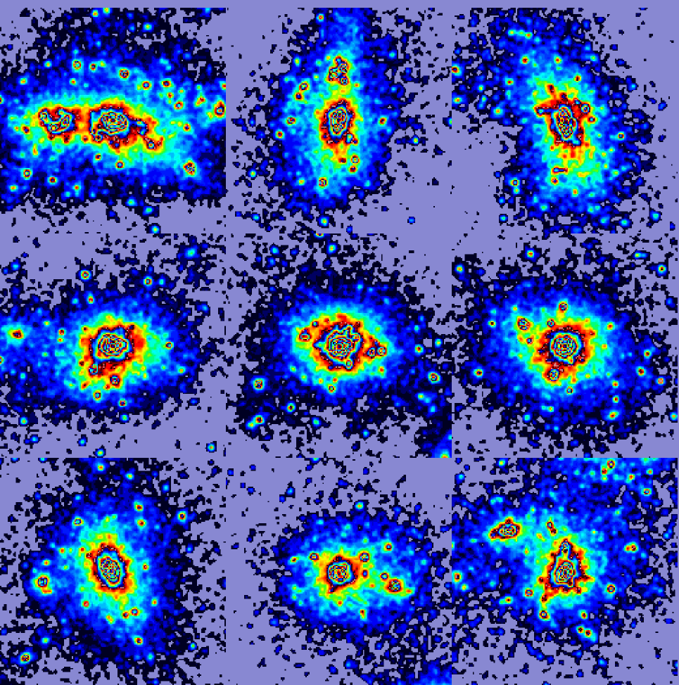
Figure 4: Projected dark matter density of the nine halos presented in this paper. Images are shown from left to right and from top to bottom following the order of Table 1. All outputs at $z=0$; the size of each image is $3R_{v}$ on a side, with $R_{v}$ the virial radius of the halo.

3 Cluster profiles: definitions and numerical tests

We want to investigate the distribution of dark matter in cluster-size halos, in particular in their central regions. We will do this mainly by showing various profiles (density, mass, velocity) obtained from the simulations.

3.1 Profile construction

We defined profiles by binning the particles in spherical shells centred on the cluster centre, as identified by the procedure described in the next Subsection.

We tried both mass weighted profiles (with shells containing a fixed number $k=25$ or $k=50$ particles), and equally spaced logarithmic intervals of width $0.1$. Since the profiles binned in equal logarithmic intervals are less noisy than the mass weighted profiles, and still let one describe the halo properties down to small radii, we use them in the figures of this paper. However, we performed some of the analysis also with mass weighted bins, and did not find significant differences in the results.

The velocity profiles were calculated as follows. First we defined the velocity reference frame by computing the mean velocity of the cluster. Such a velocity was obtained by averaging over all particles within the radius enclosing half the virial mass. We did not take all the particles in the cluster in order to exclude possible merging substructure, which would bias the mean velocity estimate. This mean cluster velocity was then subtracted from the velocity of each particle. The rms velocity within $r$ and the velocity dispersions at $r$ were computed in this reference system, that is we assumed a static non-rotating halo.

3.2 Center definition

The cluster centre was identified as the densest point of the dark matter lump, found iteratively as the centre of mass of spheres of increasingly smaller radius. We started with a radius enclosing the whole system, and stopped the iteration when a (fixed) small number of particles, say $m$, were left in the sphere. The position of the centre of mass of these $m$ particles was then identified as the final cluster centre. The center found with this procedure corresponds with very good accuracy to the highest density peak of the simulation, even in cases of ongoing merging between different lumps, and also to the position of the particle with most negative gravitational potential (Lemson 1995, Tormen 1996 in preparation). The only free parameter of this method is the number $m$ that determines when the iterative calculation should stop.

Using a few clusters in our sample, we tested that the scatter in the centre location due to different choices of $m$ is negligible. In fact, the distribution of centre positions obtained by varying $m$ from 1 to 100 has a dispersion of about 5 kpc in the tested clusters, well below the gravitational softening of the simulations. We also found that the uncertainty in the centre position leads to differences in the profiles which are perfectly compatible with the Poissonian noise in the shells. We thus defined the the centre of each of the nine clusters as the average between the centre positions found by varying $m$ from 1 to 100.

3.3 Time integration accuracy

A crucial ingredient for a reliable result, especially in the densest region of the clusters, is the accuracy of the time integrator. The use of a tree code with individual and arbitrary time steps is therefore ideal to follow with high accuracy the trajectory of particles travelling in very dense regions. The time step of each particle is set by requiring that the relative change of position and velocity of the particle be smaller than a fixed tolerance. In our standard simulations, we chose a time integration tolerance corresponding to about 15000 to 22000 time steps per Hubble time, for the minimum time step actually taken by the particles. The minimum time step allowed in principle was at least ten times smaller than this. We also set a limit on the maximum allowed time step which corresponds to 24 time steps per Hubble time. Such big jumps were taken by a few background particles at large distance from the central system.

To make sure that such accuracy is high enough to properly resolve the particles’ orbit down to the cluster centre, we ran the last $10^{9}$ years of a simulation three times, each time with different accuracy in the time integration scheme. The minimum timestep in the three cases corresponded to $100000$, $30000$ and $9000$ timesteps per Hubble time. The halo had $N_{v}=30000$ particles and a gravitational softening of 36 kpc. At the final time, we compared the profiles of the three runs: density, circular velocity, radial velocity dispersion and cumulative rms velocity, binned in logarithmic intervals 0.1 wide. We found very good agreement in all cases. Small differences in the central region of the cluster were at about $1\sigma$ level, with $\sigma$ given by the shot noise in the bins at all radii down to the gravitational softening. We conclude from this test that the standard tolerance used for our simulations allows a tracing of the particles’ trajectory that is accurate enough for resolving the structure of the clusters even in the densest part.

3.4 Gravitational softening and particle number

The gravitational softening parameter $s$ and the number of particles composing the dark matter halo within the virial radius, $N_{v}$, are two closely related parameters. For a given $N_{v}$, $s$ must be chosen big enough to maintain the collisionless evolution of the system, i.e. to avoid two-body relaxation phenomena, but small enough to reach the highest possible resolution, if one ignores cpu time limits. If one instead first fixes a value for the softening parameter $s$, then a sensible choice for $N_{v}$ is the minimum number allowing one to resolve the central regions without suffering two-body relaxation.

Several questions related to this point can be formulated. The first is: what is the maximum scale $r_{soft}$ at which effects due to the softened gravity are visible or are important in the profiles? Second: what is the minimum number of particles $N(r_{soft})$ one needs to have within such scale in order to properly resolve the halo structure down to $r_{soft}$, i.e. in order to make two-body relaxation effects negligible within the evolution time? And what is the minimum number of particles $N_{v}$ one needs to have within the virial radius of the halo in order to have $N(r_{soft})$ particles within $r_{soft}$? In this Section we will try to answer these questions by performing test simulations with different values for $s$ and for $N_{v}$. We will show results from two orthogonal tests: one fixing the particle number and varying the softening parameter, the other fixing the softening and varying the number of particles.

3.4.1 Test of gravitational softening

Let us address the first question posed above: how big is the effect of the force softening on the results. In order to answer this question we run different simulations of the same cluster, scanning the parameter space ($s$,$N_{v}$) along curves at fixed $N_{v}$. We run our test on cluster g57, the one that looks more in equilibrium both from visual inspection and from the criteria that will be given in Section 4.1. We ran 4 simulations: three have the same particle number $N$, which gives $N_{v}\approx 24000$ at the final time, but differ in the value of the gravitational softening parameter. This was taken to be $s=20$, $50$ and $100$ kpc respectively, where the $20$ kpc run refers to the standard simulation. We also ran a larger simulation of the same cluster, with $N_{v}\approx 38000$ and $s=10$ kpc, which took 32000 minimum timesteps. We will use this simulation as a reference for the all numerical tests presented in this Section. That is, we will quantify the effect of varying $s$ and $N_{v}$ by comparison to this reference simulation.

It is possible that Poissonian fluctuations in the particle counts, or transient phenomena like a subclump crossing the cluster centre, cause differences in the halo profiles. In the present test, such differences would be spurious ones, because they are not strictly due to the change of the softening parameter, and we would like to remove them from the results. Since we do not have a large number of simulations to average on, we average instead over the last few snapshots for each of the four cluster runs, under certain hypotheses of regularity. Specifically, we select, for each cluster, all the time outputs that at the same time satisfy the following two characteristics: the cluster virial mass be at least 90% of the final mass; the redshift of the cluster be less than 0.1. The first requirement minimizes possible dependence of the results on the cluster mass; the second minimizes possible evolutionary effects. In practice this means selecting the last four outputs of each simulation.

The average is performed on equally spaced decimal logarithmic intervals of width 0.1 in $\log(r)$. In this way we obtain for each cluster some average profiles, which we consider as representative of the typical dynamical configuration of the halo at recent times.

The radial profiles for density $r^{2}\rho(r)$, circular velocity $v_{c}(r)$, shell radial velocity dispersion $\sigma_{r}(r)$ and one dimensional rms velocity in spheres $v_{rms}(r)$ are shown in Figure 6. The solid line indicates the profile of the reference simulation ($s=10$ kpc). The profiles are plotted down to a radius equal to the gravitational softening, indicated by the vertical lines on the left, provided that there are at least 50 particles within the corresponding bin. The virial radius is given by the vertical lines on the right.

Figure 6: Test of gravitational softening. The solid curve refers to the reference simulation: $N_{v}=38000$, $s=10$ kpc. The other curves refer to halos with $N_{v}\approx 24000$ and $s=20$ kpc (dotted), $s=50$ kpc (dashed) and $s=100$ kpc (dot-dashed), The vertical bars on the left indicate the value of the gravitational softening for each profile. Those on the right indicate the virial radius.

Simulations with softer forces are expected to produce halos that are less dense in the centre and have lower velocities. This is clearly the trend in the figure. However, differences in the profiles at radii larger than the softening radius are of the order of 20% or less in all cases. This result answers the first question we posed above: we can trust the profiles of our standard simulations to $\sim 20\%$ or better down to a distance from the centre $r_{soft}$ equal to the gravitational softening $s$. This is quite a good accuracy, being comparable to the noise level of mass weighed profiles with 25 particles per bin, and recalling that density in halos varies over 5 orders of magnitude.

3.4.2 Test on particle number

Having found that $r_{soft}\simeq s$, we may rephrase the second question posed at the beginning of this Section as follows: how many particles are needed within a softening radius from the cluster centre in order to trust the density profiles down to $r=s$ and to avoid two-body relaxation effects?

To answer, we made another test, which is orthogonal to that just described. We run different simulations of the same cluster using the same gravitational softening $s$, but changing the particle number $N$. We hope this will give us some idea of the minimum number of particles needed to resolve the cluster down to a given scale from the centre. This set of simulations thus scans the parameter space ($s$,$N_{v}$) along curves at fixed $s$. We chose $s=20$ kpc, and particle numbers roughly corresponding to 24000, 12000 and 7000 particles within the virial radius of the halo. For this test we used the same cluster selected above, i.e. g57. We averaged the profiles from the last four time outputs, in the same way described above, to isolate the effect of particle number from transient dynamical effects.

Figure 8: Test on particle number. The solid curves refer to the reference simulation: $N_{v}=38000$, $s=10$ kpc. The other curves have all $s=20$ kpc and $N_{v}=24000$ (dotted), 12000 (dashed) and 7000 (dot-dashed). The vertical bars indicate the softening and virial radius for all simulations.

Figure 8 shows the resulting profiles. The simulations with 24000 and 12000 particles within the virial radius agree quite well with the reference run: the differences are less or of order 20% in the profiles. The run with $N_{v}\approx 7000$ instead has profiles systematically lower than the reference ones; differences at small radii are more than a factor of two in the density, of around 50% in the mass and of order 30% in the radial velocity dispersion. The least affected profile is the mean rms velocity, which differs less than 20% from the reference value. It is only at radii larger than about 100 kpc,corresponding to a sphere enclosing 250 to 300 particles, that these profiles agree with those of the other simulations.

Note that the simulation with $N_{v}\approx 7000$ has only $\approx 10$ particles within $r=s$, so there are not enough particles to reliably define the profiles down to $r=s$. We conclude that, in order to achieve a dynamical resolution of about $0.01R_{v}$, or -2 in log$(r/R_{v})$, to better than 20% in the profiles down to the softening radius, one needs at least $\approx 12000$ particles within the virial radius. This of course for the kind of models analyzed here. Equivalently, we can say that 10 particles within a radius equal to the softening radius are not enough to avoid discreteness effects in the central 100 kpc, for a cubic spline softening.

In order to confirm and extend this result we ran other sets of simulations, each set with a fixed gravitational softening and different particle numbers. In one case we took $s=36$ kpc, corresponding to log$(s/R_{v})\simeq-1.8$, and $N_{v}\approx$ 30000, 13000, 7000 and 3000. In a second set we took $s=80$ kpc, corresponding to $\log(s/R_{v})\simeq-1.5$, and $N_{v}\approx$ 2,500, 1,200 and 800. We also ran a simulation with $s=10$ kpc or $\log(s/R_{v})\simeq-2.3$ and $N_{v}=24000$ to compare to the reference simulation. Looking at the profiles resulting from all these tests we found that, in order to produce reliable profiles down to $r=s$ one needs at least $N_{v}\approx 38000$ for $\log(s/R_{v})=-2.3$, and $N_{v}\approx 7000$ for $\log(s/R_{v})=-1.8$. With $N_{v}$ smaller than these values, the profiles exhibit the same trend: a flattening of the density in the centre and lower velocities. The same profiles agree however with the reference ones at radii enclosing more than 200 to 250 particles. On the other hand, $N_{v}\approx 800$ seems enough to resolve scales down to $\log(s/R_{v})=-1.5$.

3.5 Numerical tests: Conclusion

We can summarize the results of our tests as follows.

1. The uncertainty in the halo centre is well below the value of the gravitational softening, and the corresponging errors introduced in the profiles are below the shot noise level.

2. The time integration of the simulations is performed with sufficient accuracy to ensure the correct orbit calculation for all particles, including those in the densest regions.

3. The softening of gravity at small scales causes appreciable effects only at scales below the softening $s$ itself. At scales larger than $s$ the profiles are affected by softening by less than 20% in all cases.

4. We find that, for a gravitational softening $s\simeq 0.01R_{v}$, the number of particles required to avoid discreteness effects is conservatively $N_{v}~{}\mathrel{\mathchoice{\vbox{\offinterlineskip\halign{\hfil$\reset@font\displaystyle#$\hfil\cr>\cr\sim\cr}}}{\vbox{\offinterlineskip\halign{\hfil$\reset@font\textstyle#$\hfil\cr>\cr\sim\cr}}}{\vbox{\offinterlineskip\halign{\hfil$\reset@font\scriptstyle#$\hfil\cr>\cr\sim\cr}}}{\vbox{\offinterlineskip\halign{\hfil$\reset@font\scriptscriptstyle#$\hfil\cr>\cr\sim\cr}}}}~{}10000$. Smaller numbers of particles cause a flattening of the density profile in the centre and significant differences in the results out to a radius enclosing $\approx 250$ particles.

4 Cluster formation process

We restricted our study to a specific fiducial cosmological model, namely an Einstein-De Sitter universe with zero cosmological constant and scale-free density perturbation spectrum $P(k)$ with a spectral index $n=-1$. This slope is similar to that of the standard CDM power spectrum on cluster scales. Therefore, the conclusions that we will draw from this work should also give us some insight on the formation of galaxy clusters in CDM universes.

The aim of this paper is not to compare different cosmological models, but rather to study with high accuracy the cluster formation process in a specific but representative case. For this we have many independent examples of well resolved halos coming from the same universe and from a relatively limited mass range. We can therefore estimate the expected scatter in results, for the evolution of clusters that are in principle very similar. In particular we can study the dynamics of the cluster growth, which can range from a quasi-static accretion state to violent merging events. We can also see how these states alternate during cluster evolution, and how they influence cluster dynamics.

4.1 Evolution of mass and rms velocity

Figure 10 shows, for all objects in our sample, the time dependence of the total (i.e. virial) cluster mass and of the one-dimensional rms velocity within the virial radius. At early times the most massive cluster progenitor was taken. Each panel refers to a cluster. The quantities are measured at 24 different times, except for clusters g36 and g40, for which we have stored fewer data.

Figure 10: Evolution of virial mass and rms velocity. Quantities are normalized to their value at $z=0$.

One can easily see from the trend of the virial mass that the cluster accretion process is characterized by two quite different phases. The first is recognized by sudden leaps in the mass curve, which correspond to merging events, i.e. to rather massive lumps crossing the virial radius. The number of merging events during the simulation is three to five in most cases. The mass of the merged substructure, roughly estimated by the leaps in the mass curve, can range from about 20% of the mass of the main lump to a value comparable to it. The second phase is a relaxation phase, which follows each merging event, and corresponds to periods during which the cluster does not significantly accrete, but rather processes the infallen matter. During this period, the substructures orbit within the virial radius, swing back and forth through the cluster centre and are gradually destroyed. The mass versus time curve is thus characterised, in this phase, by a plateau or by gentle growth.

Even in absence of accretion, the virial Mass of a cluster will grow, since the expansion of the universe makes the background density decrease and the nominal boundary of the cluster thus expands. A virial mass that remains constant or even decreases with time, as is sometimes observed in the plots, indicates that there is a net outflow of matter at the virial radius.

The alternation of the merging and relaxation phases is typical of all the clusters in our sample, although the length of time a cluster spends in one phase or the other varies, as can be inferred from Figure 10.

Looking now at the behaviour of the average rms velocity of particles within the virial radius, we see that the merging phase causes an increase of $v_{rms}$. This is due to the kinetic energy acquired by the subclump as it falls in the potential well of the main cluster. The rms velocity peak corresponds to the first passage of the subclump through the cluster centre, so it is slightly delayed with respect to the jump in virial mass. This finding agrees well with the results of Crone & Geller (1995).

After this first passage the rms velocity gradually decreases towards a minimum, and the cluster relaxes while it is destroying the recent acquisition. The peak value is usually $\approx 15\%$ higher than the following equilibrium value, but in some cases it is 30% higher.

The relaxation of the cluster implies a decrease of the rms velocity, whether or not there is significant substructure. In fact we stress that, from the time sequence of outputs, it is evident that only the first passage of a merger through the centre of the main cluster produces a significant rise in the rms velocity. Subsequent passages are already damped and are much slower: they do not show up in the curves. In the same way, when a merging clump has already crossed the cluster border but has not yet aquired significant kinetic energy from its fall, the rms velocity is not affected by its presence. So the presence of substructure does not, in itself, change the velocity distribution of the cluster, and a very lumpy cluster can be still relaxed from the velocity point of view. In this sense, clusters in an $\Omega=1$ universe, which are accreting up to the present day, may also go through phases of relaxation.

We may ask several questions at this point: can we show more quantitatively that this alternation of states really corresponds to changes in the system equilibrium? If so, how much is the system affected in terms of, e.g., mass estimates based on the velocity dispersion? And finally, what fraction of its evolution does the system spend, on average, in a relaxed or perturbed state? We will discuss these equilibrium issues in Section 6.1, after analysis of the halo profiles.

5 Halo profiles

In this Section we present our results for the profiles of the nine halos drawn from our $N$-body simulations. There has been much debate over the expected shape of dark matter density profiles, the link of this to the initial cosmology, and the astrophysical implications of the existence of a core in dark matter halos. Here we limit our study to one model, an Einstein-De Sitter universe with zero cosmological constant and a scale-free density perturbation spectrum with spectral index $n=-1$. However, we can test to what extent cluster-size halos in a representative model like this are compatible with the observations.

5.1 The profiles

We can think of two kinds of approaches: an everage study, where different halos (or different outputs from the same halo) are averaged to obtain some mean cluster properties, or a case by case comparison, where individual outputs from the simulations are considered in order to have an idea of how and how much the various profiles change when the clusters evolve through different dynamical states. For this reason, we will present results for the average, most relaxed and most perturbed configuration of each cluster. By average configuration we mean the one defined in the Section on numerical tests. The most relaxed and most perturbed configuration were defined using the curves of evolution of the virial mass and rms velocity in the following way. To select the most relaxed output, we looked at Figure 10 and chose for each halo the most evolved output situated at the end of a series showing at the same time a flat or smoothly increasing mass curve and an overall decrease of the rms velocity. Since the halos in our sample usually show a relaxation phase towards the end of their evolution, the snapshots thus selected usually correspond to the most evolved time ($z=0$) or to the one immediately preceding it ($z\simeq 0.01$). Two exception are cluster g51, for which we selected the output at $z=0.08$ and cluster g15, for which we chose the output at $z=0.19$. Conversely, we chose the most perturbed output as the one corresponding to a maximum in the velocity dispersion curve, following a recent merging. Here also we chose the most evolved among the possible outputs, to retain the maximum mass resolution.

Averaging over different snapshots of a cluster allows us to reduce somewhat the noise in the profiles. Since this procedure is in some sense equivalent to averaging over different clusters at the same output time, the average over different dynamical configurations of the same object will hopefully produce data which are more representative of the most likely state of a cluster, and will perhaps allow a better comparison with the observations. After all, real clusters are observed in various dynamical states, and not in their most relaxed configurations. On the other hand, the relaxed profiles are perhaps closer to our idealized theoretical models, since their dynamics should be less perturbed and more similar to a simple spherical system. Therefore one hopes that the relaxed shape of halos is more similar to the analytical predictions. We recall however that the configurations we call relaxed do not correspond to true static systems, because they usually still have a lot of substructure; accretion never stops in an $\Omega=1$ universe.

On the other hand, perturbed configurations may present the cluster under extreme non-equilibrium conditions, which are nevertheless useful to give some idea of the range of configurations one may happen to observe in the same object. Figure 12 shows the density profiles, all binned in logarithmic intervals of width 0.1.

Figure 12: Density profiles of our nine halos. For each halo we plotted three profiles, corresponding to the average (AVE: thick solid line), most relaxed (REL: thin solid line) and most perturbed (PER: dotted line) dynamical configuration. Straight lines correspond to asymptotic logarithmic slopes $-1$ and $0$ at small radii and $-3$ and $-4$ at large radii.

On average, the density profiles of the three kinds show the following features: a steeper logarithmic slope at large radii, an intermediate region where the slope bends towards the singular isothermal sphere value $-2$, and finally an inner region where the profile becomes gradually flatter. Sometimes at intermediate radii the profile follows almost a power law; sometimes the change of slope is more gradual and relatively smooth. The spikes visible in many clusters at large radii correspond to merging objects which have just crossed the cluster virial radius.

We see that, in general, the three profiles of each cluster are fairly similar. Only two clusters (g15 and g66) show significant differences, of the order of a factor of 2, between the averaged, relaxed and perturbed density profiles. The other halos have profiles which differ by roughly 20% in the averaged and relaxed configurations, or 40% including the perturbed outputs. This differences are not big, and the result tells us that the halo density, once averaged in spherical shells, is not a very sensitive measure of dynamical evolution.

Figure 14: Circular velocity profiles for the nine halos. Line types are as in Figure 12.

The same comparison is made for the circular velocity profiles in Figure 14. Here the general trend is a rising circular velocity at small radii, a maximum and then a decrease at large radii. The departures from the isothermal behaviour $v_{c}=const$ are not due to limited resolution, but are real as was demonstrated in the Section dedicated to numerical tests. In particular, the decrease at large radii always starts well within the virial radius of the clusters. Differences between the various configurations are smoother here, since their effect is integrated over the cluster. Again the averaged and most relaxed profile agree quite well, and also the perturbed outputs show average differences of roughly 20%, but up to 60% for the two cluster mentioned before.

The average one dimensional rms velocity within spheres of radius $r$, for the three configurations and for each cluster, are plotted in Figure 16. The profiles show an rms velocity that is usually increasing with radius at small $r$, but sometimes is flat. After reaching a maximum, $v_{rms}$ decreases slowly at large radii. Cluster g66 exhibits a larger difference between the three configurations because it shows a merger passing through its centre in the perturbed and averaged profile.

Differences between the perturbed and relaxed configuration usually are of the order of 15% at the virial radius; in two cases they are as big as 30% to 40%. A naïve application of the Virial Theorem would therefore miss the true mass of the halo by 30% on average. We will come back to this point in more detail in Section 6.1.

Figure 16: One dimensional rms velocity within spheres of radius r, for our halos. Lines are as in Figure 12.

The radial velocity dispersion $\sigma_{r}(r)$ for the nine halos follows the behaviour of the rms velocity, rising with $r$ at small radii and decreasing at large radii. In this case the curves are more noisy and the curvature more pronounced because $\sigma_{r}(r)$ is computed for each shell while $v_{rms}$ is averaged on all particles within $r$. The halos are thus not generally isothermal. However, departures from the isothermal model are not very big, at least for the averaged or relaxed outputs: the typical variation in radial velocity dispersion over the range of radii resolved by the simulations ranges from about 45% for the averaged and relaxed configuration to about 70% for the most perturbed outputs.

Lastly we show in Figure 18 the behaviour of the velocity anisotropy parameter, $\beta(r)=1-\sigma_{t}^{2}(r)/2\sigma_{r}^{2}(r)$, where $\sigma_{r}(r)$ and $\sigma_{t}(r)$ are the radial and tangential velocity dispersion, and the tangential velocity of each particle is defined by $\sigma_{t}^{2}=v^{2}-\sigma^{2}_{r}$. A value $\beta(r)=1$ means purely radial orbits at that radius; an isotropic velocity field has $\beta(r)=0$, while $\beta(r)<0$ means a predominance of tangential motions.

Each panel shows $\beta(r)$ for all halos together. The left panel refers to the averaged outputs, the central to the most relaxed ones, the right panel to the most perturbed outputs. Although the scatter in the quantity is different, the trend is the same in all cases: $\beta(r)\simeq 0.2$ for $r\leq 0.2R_{v}$, then it steadily increases with $r$, and reaches $\beta(r=R_{v})\simeq 0.6$. Radial motion predominates at large radii, while in the inner part of the halo orbits are more nearly isotropic. The transition between these two regimes happens at around one fifth of the virial radius. In one case (halo g87) the velocity field is more isotropic also at large radii.

The results for $\sigma_{r}(r)$ and $\beta(r)$ are in good qualitative agreement with those of Crone et al (1994) and Cole & Lacey (1996), although the value of $\beta(r)$ we find is slightly larger than theirs. In their model of cluster A2218, Natarajan & Kneib (1996) find a negative $\beta(r)$ at small radii; although in contrast with our average result, Figure 18 shows that $\beta<0$ can occasionally be measured.

Figure 18: velocity anisotropy parameter (defined in the text). In each panel the profiles from all nine halos are plotted. Left panel refers to averaged outputs, central panel to most relaxed outputs, right panel to most perturbed outputs.

5.2 Analytic fits to the profiles

In this Section we present possible analytic fits to the profiles we have just shown. We will show results of the analysis performed on the averaged profiles, as their features are similar to those of the most relaxed ones. We will however present the conclusions also for the most relaxed outputs. We will not consider the perturbed profiles in what follows.

We should first ask what is the purpose of an analytic fit. Viewed as a data compressing technique, one may want to find a fitting function that gives a good overall description of the observed profile at all radii, regardless of its true dynamical significance. However, at a deeper level one might also hope that the analytic fits have some real dynamical meaning. In this paper we deal with the first approach only.

From Figures 12 to 16 it is clear that the density and circular velocity profiles are not well represented by a single power law: they may exhibit a power-law behaviour at some radii, but this does not extend throughout the cluster. The departures from a single power law, at small and large radii, are real and are not due to numerical inaccuracies, as we showed in Section 3. We will thus limit our comparison to curved fits. In particular, we are going to consider the analytic profile recently proposed by NFW and the HER profile. Both describe the density profiles as a curve with a single scale radius that sets the scale of transition between two power laws. These profiles have been presented in the Introduction; we recall their form here:

NFW fit:

$$\rho(x)=\rho_{0}x_{s}^{3}{1\over x(x+x_{s})^{2}};$$ (1)

HER fit:

$$\rho(x)=\rho_{0}x_{s}^{4}{1\over x(x+x_{s})^{3}};$$ (2)

where $x=r/R_{v}$, and $x_{s}=r_{s}/R_{v}$, with $r_{s}$ the scale radius of the fit. The value of $\rho_{0}$ is determined by imposing that the mean density within $R_{v}$ is $178$ times the mean background density. The corresponding circular velocities are:

NFW:

$$v_{c}^{2}(x)=4\pi\rho_{0}R_{v}^{2}x_{s}^{3}G\left[{1\over x}\ln(1+{x\over x_{s}})-{1\over x+x_{s}}\right];$$ (3)

HER:

$$v_{c}^{2}(x)={GMx\over R_{v}(x+x_{s})^{2}},$$ (4)

where $M$ is the total mass of the system.

Both profiles have the same asymptotic behaviour at small radii: $\rho(r)\propto r^{-1}$ as $r\to 0$. The difference between them is at large radii, where the NFW profile is shallower, with $\rho(r)\propto r^{-3}$ as $r\to\infty$. The HER profile instead behaves as $\rho(r)\propto r^{-4}$ at large radii. In the range of interest, i.e. for $0.01\mathrel{\mathchoice{\vbox{\offinterlineskip\halign{\hfil$\reset@font\displaystyle#$\hfil\cr<\cr\sim\cr}}}{\vbox{\offinterlineskip\halign{\hfil$\reset@font\textstyle#$\hfil\cr<\cr\sim\cr}}}{\vbox{\offinterlineskip\halign{\hfil$\reset@font\scriptstyle#$\hfil\cr<\cr\sim\cr}}}{\vbox{\offinterlineskip\halign{\hfil$\reset@font\scriptscriptstyle#$\hfil\cr<\cr\sim\cr}}}}r/R_{v}\mathrel{\mathchoice{\vbox{\offinterlineskip\halign{\hfil$\reset@font\displaystyle#$\hfil\cr<\cr\sim\cr}}}{\vbox{\offinterlineskip\halign{\hfil$\reset@font\textstyle#$\hfil\cr<\cr\sim\cr}}}{\vbox{\offinterlineskip\halign{\hfil$\reset@font\scriptstyle#$\hfil\cr<\cr\sim\cr}}}{\vbox{\offinterlineskip\halign{\hfil$\reset@font\scriptscriptstyle#$\hfil\cr<\cr\sim\cr}}}}1$ the HER profile is the most curved of the two, because the difference between the two power laws is larger.

We have fitted the profiles of our nine dark matter halos with both analytic models. The best fit was determined using the logarithmic density profile. Because the circular velocity is an integrated estimate, the limits on resolution at small scale influence the profile at larger radii than is the case for the density. The minimization was performed by a standard Chi Square method in the range $s\sim 0.01R_{v}\leq r\leq R_{v}$ (with $s$ the softening radius). We used profiles binned in equally spaced logarithmic intervals of width 0.1, as described above. As a result, our fit is not mass weighted, but gives equal weight to small and to large radii.

Figure 20: The averaged (AVE) density profiles of the nine halos (thick solid curves) are plotted with the best fitting analytical models. Dotted curves are NFW profiles, dashed curves are HER profiles.

Figure 22: Circular velocity profiles for the AVE configuration of our simulations plotted with the best fitting NFW and HER profiles. Line types are as in Figure 20.

Figure 24: Residuals of the fits to the AVE profiles of the previous two figures.

Figures 20 and 22 show, for the averaged configuration, the density and circular velocity profiles respectively, and their best NFW and HER analytical fit. The thick solid curve is the actual profile of the simulated halo, the dotted curve is the best fitting NFW profile, and the dashed curve is the best fitting HER profile. Recall that the fit has been made on the density profiles. Therefore in some cases the best-fitting curve for the density does not correspond to the best-fitting curve for the circular velocity.

Figure 24 shows a summary of the fitting results. It refers to the averaged profiles, and plots the residuals of both the NFW and HER profiles for the density and circular velocity. One can see that on average the density profiles of the simulated clusters look steeper than both analytical fits at small radii, and shallower than the HER fit at large radii. Part of the positive residuals at large radii may be due to the presence of merging subclumps. The scatter ($1\sigma$ dispersion) in the residuals is smaller for the NFW profile, and larger for the HER profile, 17% and 26% in density, respectively. The circular velocity is fitted with smaller scatter, 6% and 10% for NFW and HER respectively. If we consider the fact that the curves extend over two orders of magnitude in radius, and over four orders of magnitude in density, both fits can be considered quite good. The NFW model fits our simulations on average 50% better than the HER model, down to at least $r\simeq 0.01R_{v}$. Since the simulated profiles are in general less curved than either of the models at intermediate radii, the maximum circular velocity estimated by the fits is generally bigger than the true one, although the difference is small.

One can repeat the same kind of analysis on the most relaxed outputs of each halo. The corresponding residuals have however a larger scatter: the $1\sigma$ dispersion in their distribution is 24% and 34% for the density fits, for the NFW and HER models respectively, and 10% and 12% for the circular velocity fits. Therefore the averaged profiles turn out to be slightly better fitted by the analytic curves than the relaxed profiles. We are somewhat surprised by this result, and would have expected the converse. It may be that the bigger intrinsic noise in the relaxed profiles (which are built from only one output) is responsible for the bigger deviations. At any rate, differences between the averaged and most relaxed profiles are small.

5.3 In search of equilibrium

We want to push the equilibrium issue a bit further. That is, we would like to know how the halo characteristics would change with respect to those measured so far, if the system reached a real dynamical equilibrium, and all substructure was processed and destroyed. Since this cannot happen in an Einstein-de Sitter universe, where galaxy clusters are dynamically young and accretion goes on for ever, we have to break the clustering hierarchy in some way, and then let the halos relax.

For this purpose we made the following experiment. We chose the last output of each simulation, corresponding to the present time, and removed from it all the particles beyond a fixed radius $R_{cut}$ from the cluster centre. We choose $R_{cut}\simeq 2R_{v}$. We then evolved the remaining particles, that is those forming the halo out to $R_{cut}$, with void boundary conditions around it, for another Hubble time. By cutting the halos at twice their virial radius we allowed some additional infall of surrounding matter. We hope that the evolved clusters will get at least closer to the ideal configuration of perfect equilibrium with no perturbing substructure. The fact that we are missing part of the infalling matter should not affect the profiles at very small scales,but might cause some steepening in the outer parts of the density profiles.

At $t=2t_{H}$ we repeated the fitting analysis performed on the original clusters. In order to obtain a mean evolved profile we averaged the last four outputs, corresponding to times from $t=1.875t_{H}$ to $t=2t_{H}$. We will name these profiles EVO (for evolved). On these we tried again both the NFW and HER fits. We noticed that the density profiles of most halos tend to flatten at very small radii as we evolve them beyond $t_{H}$. It is likely that this effect is due to collisional relaxation, or to the inaccuracy of the force evaluation of the code. We therefore decided not to use the very inner part of the profiles in the fitting procedure. Specifically, the fits have been made only at radii larger than the radius enclosing 500 particles. The density and circular velocity profiles of the evolved halos, together with the best fits for the NFW and HER models are presented in Figures 26 and 28.

Halos evolved until $t=2t_{H}$ look much more dynamically relaxed than the original ones: very little substructure has survived within the virial radius. Moreover, the power law density profiles exhibited at intermediate radii by some halos in the previous configurations have disappeared, and all halos have now smoothly curved profiles. The residuals of the fits are shown in Figure 30. The scatter in the residuals is lower than before for the density, and about equal for the circular velocity; considering all the points down to the softening radius, the $1\sigma$ dispersion is 14% (NFW) and 20% (HER) for the density, and 7% (NFW) and 10% (HER) for the circular velocity. The improvement in the density fit shows that part of the scatter was due to the presence of substructure; as a halo approaches dynamical equilibrium its density is more accurately described by the NFW and HER profiles. We conclude from this test that the NFW and HER models are indeed good fitting formulae for the equilibrium configuration of the density and circular velocity of our dark matter halos.

Figure 26: The evolved (EVO) density profiles of our simulations are plotted with their best fitting analytical NFW and HER models. Lines are as in Figure 20. Only the fitted range of each profile (that is for radii larger than the radius enclosing 500 particles) is shown.

Figure 28: Circular velocity profiles for the EVO outputs together with their best fitting analitical NWF and HER profiles. Only the fitted part of each profile is shown.

Figure 30: Residuals of the fits to the EVO profiles in the previous two figure.

5.4 Trend with mass

In their N-body simulations of CDM dark matter halos, NFW recently found that more massive halos appear less centrally concentrated than less massive ones. NFW interpret this trend in terms of a dependence on the mean density of the universe at the time of halo formation, defined as in Lacey & Cole (1993). The trend they find is weak, and requires a large range of halo masses in order to be properly detected. CL found a similar trend for the scale radius of their halos, formed in scale-free Einstein-de Sitter universes of the kind we are discussing.

In Figure 32 we show the result of the same test on our halos: the normalized scale radius $x_{s}$ is plotted versus the halo mass. Masses are normalized by the characteristic mass $M_{*}$, which is naturally defined at every time as the linear mass on the scale currently reaching the non-linear regime:

$$M_{*}(t)={4\over 3}\pi R_{*}^{3}\rho_{b}(t).$$ (5)

In the equation $\rho_{b}$ is the mean density of the universe, and $R_{*}$ is such that the linear density contrast on scale $R_{*}$ is $\delta(R_{*})=1.69$, the linear extrapolation to the collapse of a spherical top-hat. Recalling that the mass variance goes as $\delta_{M}\propto R^{-(3+n)}$ for a scale free power spectrum $P(k)\propto k^{n}$, and with our current normalization $\delta_{M}(8h^{-1}$ Mpc$)=0.63$, the value of $M_{*}$ for our simulations is $M_{*}=6.16\times 10^{13}$ M${}_{\hbox{$\odot$}}$ at the present time (for $h=0.5$).

Open squares refer to our results; each number labels a halo. The first three rows show points corresponding to the AVE, REL and EVO configuration; the last row plots all points together. The black circles refer to simulations of a $n=-1$ scale free Einstein-De Sitter universe (Navarro 1996), while the black squares are the results of CL. Note the wider mass range covered by the Navarro (1996) results. Our data show that indeed more massive halos have a larger scale radius, but since they cover a limited mass range we cannot make a very definite statement on the slope of the relation. The solid lines are the best fit to the points in each panel. The dotted line is the best fit to the AVE points, repeated in all panels to show how this is also a reasonable slope for all configuration. Its value is $0.4$ and $0.3$ for the NFW and HER points respectively.

For a given halo mass there are significant variations in the value of $x_{s}$ both within the same configuration and between different configurations. For the combined data the $1\sigma$ dispersion in scale radius is $14\%$ (NFW) and $11\%$ (HER). This means that halos best fit by the same model profile can differ in mass by a factor of two at a $2\sigma$ level. Given this scatter, the points from Navarro are in good agreement with ours in the range tested by our simulations. The points from CL instead are systematically higher: their halos seem less centrally concentrated than ours, and our relation is slightly steeper than theirs. Such a discrepancy could be due to the lower force and mass resolution of the simulations used by CL: as a consequence, they did not push the fit to radii as small as ours. To test this possible explanation, we repeated the fit on our average profiles two more times, using for the fit the narrower ranges $\log(r/R_{v})\in[-1.5,0]$ and $\log(r/R_{v})\in[-1,0]$; these choices bracket that of CL. We found that limiting the fit in this way does indeed cause generally higher estimates for the scale radius, so we could marginally match the points of CL. We also found that fitting a narrower portion of the profiles causes a bigger scatter in the relation, to the point that, in the case $\log(r/R_{v})\in[-1,0]$, most of the correlation between $r_{s}$ and mass was lost in our sample. Our understanding of this effect is the following. In limiting the fit to the outer part of the profile one becomes more and more sensitive to density enhancements at $r\approx R_{v}$, caused by merging substructure. These will both add noise and flatten the density profiles and thus will bias the fit towards higher values of scale radius and worsen the correlation with the halo mass.

A concurrent possibility for the discrepancy between us and CL could be that our halos have, perhaps, different average dynamical configurations than halos in the CL sample. To test this we repeated the fit using the most perturbed configuration of each halo: we did find a somewhat bigger scatter in the value of $r_{s}$ at low masses, but the overall trend came out similar to that found for the AVE and REL configurations. Further reasons could be the different criteria used to select the halo centres and the best fitting value of $x_{s}$, or the fact that the number of timesteps used to evolve the simulations of CL may be too small to properly integrate orbits near the cluster centre. Finally, we also tried to first average the density profiles $\rho(r/R_{v})$ of halos of similar mass, and then fit the result with the analytical models, as CL do, but found no difference in our results.

To test the consistency of our results, we may use the fact that our halos come from a self-similar universe. Therefore, we should be able to reproduce the relation between scale radius and halo mass using halos picked up from less evolved outputs. We limited our choice to all outputs with $z<0.5$, to retain sufficient mass and force resolution (we recall that our gravitational softening is fixed in proper coordinates, so that e.g. at $z=0.5$ the profiles are resolved down to $\log(r_{min}/R_{v})\simeq-1.5$). We found that, on average, less evolved halos require larger values for the scale radius; however, the difference between these and the results shown in Figure 32 is consistent with the effect expected by fitting on a narrower range of radii, as explained above.

From these tests we conclude that indeed more massive halos have on average flatter density profiles than less massive ones. Although our mass range is only roughly a factor of six, the trend is statistically very significant: a Spearman rank correlation test shows in fact that the probability of a chance correlation for our points is 0.4%, 0.2%, 4.3% for the AVE, REL and EVO data, and less than 0.1% for the combined data. The relation suffers from a moderately large scatter due both to changes in the halo dynamics and to fluctuations in the halo population. This fact, and the scatter between the present and previous results, make a precise determination of this relation difficult. For these reasons, we think that further study is needed before using it for applications.

Figure 32: Trend of the scale radius $x_{s}$ versus the normalized mass of the halos, for different dynamical configurations. Left panels refer to the NFW profile, right panels to the HER profile. Note the wider mass range in the left panels. The meaning of different symbols and curves is given in the text.

6 Other topics

6.1 Dynamical Equilibrium and mass estimation

We will now discuss the issue of equilibrium put forward in Section 4.1. Do our halos reach dynamical equilibrium? And how does merging affect this equilibrium and the mass one estimates using the equilibrium hypothesis?

To answer this we use the Jeans’ equation for the dynamical equilibrium of a collisionless system. For a static spherical system, it takes the form:

$${d\over dr}\left[\rho(r)\sigma^{2}_{r}(r)\right] + {\rho(r)\over r}\left[2\sigma^{2}_{r}(r)-\sigma^{2}_{t}(r)\right]$$ (6)

$$= -{G\rho(r)M(r)\over r^{2}(1+\epsilon^{2}/r^{2})^{3/2}}$$

where $G$ is Newton’s constant, $\rho$ is the density at distance $r$ from the cluster centre, $\sigma_{r}$ is the radial velocity dispersion and $\sigma_{t}$ is the tangential velocity dispersion defined above. The extra factor $(1+\epsilon^{2}/r^{2})^{3/2}$ takes into account the fact that the Newtonian force is softened at small radii; to first order we approximated the spline softening with a Plummer softening $\epsilon=s/1.4$. Solving for the mass gives

$$M_{E}(r)= - {r\sigma_{r}^{2}(r)(1+\epsilon^{2}/r^{2})^{3/2}\over G}$$ (7)

$$\times \left[{d\ln\rho\over d\ln r}+{d\ln\sigma_{r}^{2}\over d\ln r}+2\beta(r)\right],$$

where $\beta(r)$ is the anisotropy parameter defined above. We called the mass $M_{E}(r)$ because it is an estimate of the true mass within $r$. We can compute the rhs of Equation (7) numerically, and compare $M_{E}(r)$ with the actual mass at different radii. Moreover, we can make different assumptions or approximations by dropping one or more terms. This measures the sensitivity of the result to each term and quantifies the error made in estimating the true cluster mass.

The simplest form of Equation (7) is obtained if we approximate the halo as a Singular Isothermal Sphere (SIS):

$$M_{E1}(r)={2rv_{rms}^{2}(r)(1+\epsilon^{2}/r^{2})^{3/2}\over G}.$$ (8)

We allow the one dimensional rms velocity $v_{rms}^{2}\equiv\sigma_{r}^{2}$ to vary with $r$ as in Figure 16, and so use a different SIS at each radius. This expression in some sense is nothing more than the Virial Theorem, in that it relates the potential energy of the system to its kinetic energy.

As a second estimate we assumed a non-singular Isothermal Sphere, and used the actual slope of the density profile:

$$M_{E2}(r)=-{rv_{rms}^{2}(r)(1+\epsilon^{2}/r^{2})^{3/2}\over G}{d\ln\rho\over d\ln r}.$$ (9)

We can go further, and drop the isothermal approximation, still assuming that the velocity field is isotropic. In such a case Equation (7) reduces to

$$M_{E3}(r)=-{r\sigma_{r}^{2}(r)(1+\epsilon^{2}/r^{2})^{3/2}\over G}\left[{d\ln\rho\over d\ln r}+{d\ln\sigma_{r}^{2}\over d\ln r}\right];$$ (10)

finally, we used the complete expression Equation (7), that is we assumed a general static and non rotating spherical system, with anisotropic velocity dispersion, and call it $M_{E4}$. All these estimates rely on the assumption of spherical symmetry, which is not a very good approximation in at least half of our halos. Therefore, the results that we obtain here give only a rough idea of the role that equilibrium itself, and each term of Equation (7), play in the estimation of the halo mass.

We first verified the Jeans’ equation on the average profiles, shown in Section 5.1. The idea is that different times have roughly the same dynamical importance, and that small variations between profiles are mostly due to transients in the cluster evolution. To keep to a minimum the noise introduced by the numerical evaluation of the two derivatives, we smoothed the estimations with a Gaussian filter of logarithmic width 0.1. The results of the four estimates $M_{E}$ are shown on the first column of Figure 34; each number labels a halo.

Figure 34: Test of the halo dynamical equilibrium. The ratio of the mass estimated by the Jeans’ Equation $M_{E}$ to the true mass $M_{T}$ is plotted versus the radial coordinate. Each line refers to a different estimator (explained in the text), and each column to a different dynamical configuration. Data for all halos are plotted in each panel, labelled by number. The solid lines show the distribution mean values.

The main points to note are:

1. The analytically most accurate estimate, $M_{E4}$, shows that the dark matter halos are in reasonably good dynamical equilibrium at least within roughly one third of the virial radius. At larger radii the estimate is still fairly good but becomes more noisy due to the spikes produced on the density profiles by infalling matter. At the virial radius the ratio between the estimated and true mass is $M_{E4}/M_{T}=1.1\pm 0.38$ ($1\sigma$ of the distribution). At very small radii the noise is just Poissonian.

2. Neglecting the velocity anisotropy makes the mass estimate larger than the true mass, especially at large radii where $\beta(r)$ is significantly non zero due to predominance of radial orbits. The large scatter in $M_{E3}$ and $M_{E4}$ is partly due to the noise introduced by the numerical differentiation.

3. Although the SIS model gives wrong results at most radii, the ratio $M_{E1}/M_{T}$ follows a clear trend crossing one around the virial radius. The different approximations in this estimate seem to introduce errors which balance one another at the cluster boundary, where this form of the Virial Theorem turns out to be quite accurate. The mean ratio at the virial radius is in fact $M_{E1}/M_{T}=1.04\pm 0.08$.

4. Using the actual density slope in the isothermal model does not improve the simple SIS estimate. Although at small radii $M_{E2}$ moves in the right direction, at large radii it does not, and in general the true mass is overestimated everywhere but in a narrow region at intermediate radii.

We now ask how these estimates $M_{E}$ would change if we applied them to different dynamical configurations of the clusters. For example, we might expect a mass estimate made on a relaxed configuration to be more accurate and less noisy than an average estimate, or an estimate made on a perturbed state to be higher than the true mass, and also to have a larger scatter. To test this we repeated the same analysis using for each cluster the most relaxed and the most perturbed outputs, defined in Section 5.1, and also using the evolved outputs presented in Section 5.3. The result is shown in the second, third and fourth columns of Figure 34.

Here we can note the following things.

1. All $M_{E}$ give similar results when applied to the averaged or to the most relaxed outputs. However, in the latter case they are slightly but systematically lower. They are also slightly noisier, probably because obtained from just one profile. The SIS model is still good at the virial radius.

2. All the estimators deal significantly worse when applied to the most perturbed outputs. Departures from dynamical equilibrium cause a general overestimation of the true mass, due to the higher velocity dispersion; the scatter in the measures is also larger. However, $M_{E4}$ is still fairly consistent with the true mass, due to the large estimation noise. The SIS model fails in this case: $M_{E1}$ and $M_{T}$ differ by more than $1\sigma$.

3. The halos evolved to $2t_{H}$ are indeed in very good dynamical equilibrium: the estimate $M_{E4}$ is in excellent agreement with the true mass at all radii, with very small scatter. At the virial radius the estimate is $M_{E4}/M_{T}=1.05\pm 0.05$. This tells us that the assumption of a spherical system is actually a very good approximation for this problem. The SIS estimate is again accurate at the virial radius, with $M_{E1}/M_{T}=0.98\pm 0.07$.

4. Velocity dispersion anisotropies are important at all radii. Neglecting them leads to an average mass overestimation of 30%.

Of course in real clusters many facts make a comparison like this more difficult. We used three dimensional profiles instead of projected ones, and did not include any of the observational errors present in the data. Moreover, in true clusters one observes the galaxy distribution, which may well not be tracing the underlying dark matter potential. Nevertheless, we believe that the test we performed here is still very instructive, since it can give us some insight of how the dynamical properties of halos can change during its formation, and to what extent simplifying approximations on the halo structure may be justified.

We may now ask what is the relative occurence of different dynamical configurations in the cluster formation process: how often are the halos relaxed? Or perturbed? We can roughly estimate this by looking at Figure 10. We saw that the virial rms velocity of the halos reaches a peak during each merging event, and decreases to a minimum after it. Let us count as perturbed all the outputs which, during a major merging event, have an rms velocity closer to the peak value than to the following minimum. Analogously, let us count as relaxed the other outputs. From the figure we can roughly say that our dark matter halos spend 64% of their time being relaxed and the other 36% of the time being perturbed. This means that a mass estimate done with one of the above estimators will be likely biased upward with a probability of one third. The values shown in the third column of the figure should be regarded as a very rough upper limit, since they were computed on the most perturbed outputs only.

6.2 Consequences on Cosmology: Gravitational Lensing

An interesting application of the present study is the comparison of the mass and density profiles of the simulations with those coming from observations of weak and strong gravitational lensing in rich clusters of galaxies. In particular, since the profiles are resolved down to few tens of kpc from the centre, these simulations can be compared to the mass estimates at very small radii provided by giant arcs.

To compare the observed mass estimates to the simulated halos, we considered the simulations at different times, and selected from each output the high resolution particles forming the halo and the central part of the simulation. These particles were projected 100 times along random lines of sight (l.o.s.), and projected profiles were computed in equally spaced logarithmic bins, following the same procedure used for the radial profiles. The mean values and dispersions in each bin of the profiles were finally computed. In this procedure we neglected the low resolution particles that provide the tidal field of the simulations. Since the high resolution particles usually provide most of the mass out to two to three times the halo virial radius, neglecting the background particles has a negligible effect on the projected quantities, as we verified.

We did not constrain the simulated halos to have the same velocity dispersion $\sigma_{los}$ as the observations for two reasons. First, the observed velocity dispersion is often computed as the best fit to some model (isothermal halo, $\beta$ model or others) and so is not measured in the same way as done for the simulated halos. Second, we want to leave $\sigma_{los}$ as a free parameter, in order to give a very crude estimate of the total mass and velocity dispersion of the observed cluster based on the shape of their profiles. We show in Figures 36 and 38 the halos providing, by eye, the best fit to the observations.

Figure 36 shows in each panel the mass profile of the rich cluster A2218, as inferred from different observations (details are given in the Figure Caption). The weak lensing measure is only a lower limit on the mass, and in fact it falls slightly lower than the other estimates. These observations are compared to four outputs of the simulations (indicated by the thin error bars), two from each of the two most massive halos in the simulations The error bars are centred on their mean projected mass, and enclose $\pm 1\sigma$ of the distribution of the 100 projections. The line of sight velocity dispersion measured within the Abell radius ($R_{Ab}=3$ Mpc), for the four outputs shown, are, from left to right and from top to bottom: $\sigma_{los}(R_{Ab})=1240$, $1230$, $950$, $950$ km s^-1. The observed estimate for A2218 is $\sigma_{los}=1370$ km s^-1, but it refers to a smaller central region.

A better fit to the data is provided by the simulations in the upper panels, which come from a more massive halo and correspond to perturbed dynamical configurations. The Abell mass (i.e. the mass within a sphere of radius $R_{Ab}$) of these two outputs is equal to their virial mass and is of order of $M_{Ab}\simeq 2.2\times 10^{15}M_{\hbox{$\odot$}}$. The projected mass within the Abell radius is slightly bigger: $M=2.5\times 10^{15}M_{\hbox{$\odot$}}$. The simulations in the lower panels fail instead to match the weak lensing lower limit on the mass at $\approx 1$ Mpc. The Abell mass (projected mass) for the halos in the lower panels is $M_{Ab}=1.35\times 10^{15}(1.8\times 10^{15})M_{\hbox{$\odot$}}$ (left) and $1.5\times 10^{15}(2.1\times 10^{15})M_{\hbox{$\odot$}}$ (right). If we believe that the simulated halos are a reasonable representation of a bright cluster like A2218, then their projected Abell mass can give an idea of the mass of A2218: $2\times 10^{15}M_{\hbox{$\odot$}}\leq M_{Ab}(A2218)\approx 2.5\times 10^{15}M_{\hbox{$\odot$}}$.

In Figure 38 we plotted the projected density profiles observed for the two distant clusters 1455+22 ($z=0.26$, solid squares) and 0016+16 ($z=0.55$, solid circles). The measures come from weak lensing observations, and the normalization is not given. Therefore we only tried to fit the shape of the profile and chose the appropriate normalization in each panel. Even so, we can roughly guess the total mass and $\sigma_{los}$ of these clusters by using the fact that halos of different mass have profiles with different shape, as shown in Section 5.4. The error bars have the same meaning as in the previous figure, and they now refer to outputs from three different halos.

The velocity dispersion of the two upper halos is $\sigma_{los}=720$ km s^-1 (left) and $\sigma_{los}=1070$ km s^-1 (right). Their Abell mass (projected mass) is respectively $M_{Ab}=8.0\times 10^{14}(8.4\times 10^{14})M_{\hbox{$\odot$}}$ and $M_{Ab}=1.5\times 10^{15}(1.6\times 10^{15})M_{\hbox{$\odot$}}$. Although these values differ by almost a factor of two, their profiles fit equally well the observed profile of 1455+22, since the error bars on the observations are typically a factor of five. Their mass can perhaps bracket the mass of this cluster. In the lower panels the simulations match instead cluster 0016+16. The velocity dispersion of the halos are $\sigma_{los}=1230$ km s^-1 (left) and $\sigma_{los}=1150$ km s^-1 (right), similar to that estimated for the cluster. Their Abell mass (projected mass) is respectively $M_{Ab}=2.2\times 10^{15}(2.5\times 10^{15})M_{\hbox{$\odot$}}$ and $M_{Ab}=2.4\times 10^{15}(2.8\times 10^{15})M_{\hbox{$\odot$}}$. Again these can give an order of magnitude estimate of the total mass of the cluster.

Figure 36: mass profiles for A2218 plus four profiles from simulations. The observed profile is repeated in each panel: the solid curve is a mass model inferred by combined arc and arclets observations (Kneib et al. 1995). The triangle is an estimate from a giant arc (Miralda Escudè & Babul 1995). The solid squares come from a weak lensing model (Squires et al. 1995). The error bars indicate the $\pm 1\sigma$ of the distribution of 100 random projections of a simulated halo. The upper panels used two different outputs of halo g15, the lower panels two outputs of halo g36.

Figure 38: Projected density profiles for 1455+22 (squares) and 0016+16 (circles) in each panel, plus four different projected simulations. The data come from weak lensing observations (Smail et al. 1995). In the two upper panels the simulated halos try to match the lower observed curve; viceversa in the lower two panels. Normalization of the projected density is arbitrary. Only the shape is to be considered. Simulation outputs are taken from halo g57 and g51 in the upper panels, and from halo g15 in the lower panels.

7 Summary and Conclusions

In this paper we have used high resolution $N$-body simulations to study the structure and dynamical evolution of the dark matter halos of galaxy clusters.

Firstly we performed extensive numerical tests of some parameters that define the simulation setup and determine the resolution of the results. These are the number of particles forming the final halo, the gravitational softening parameter $s$ which sets the small scale cutoff of gravity, and the tolerance parameter that determines the accuracy of the time integration of the system. From these tests we could assess the accuracy limits of our simulations, and so choose parameter values appropriate to the dynamical resolution we required. We then obtained a set of nine dark matter halos, resolved on average by $\approx 20000$ particles each, with an effective force resolution of $\simeq 25$ kpc.

We studied the formation process of these halos and discussed their dynamical equilibrium and departures from this equilibrium during their evolution. We analyzed the density and velocity field of the dark matter, especially in the central region of the halos, by using radial profiles of these quantities. We tried two analytical fits to these profiles, and estimated their performance and range of applicability. Under different approximations for the dynamics of the system, we tested the accuracy of the Jeans’ equation in estimating the halo mass within different radii. We finally compared the dark matter profiles of the simulated halos to those inferred from recent observations of gravitational arcs, arclets and background distortions in rich clusters of galaxies.

Our main results are the following.

1. The halo formation process can be simply schematized as an alternation of merging phases and relaxation phases. Halos spend on average one third of their evolution in perturbed configurations, and the lasting two thirds in relaxed configurations. During merging the halo increases its total mass by $20\%$ to $100\%$; its velocity dispersion also increases by $\approx 15\%$ to $40\%$ due to the velocity of the infalling lumps. After the first passage of a lump through the centre of the main halo, the latter starts to relax, the velocity dispersion decreases towards its equilibrium value, and substructure is erased. During these phases, halo densities can vary by up to a factor of two, circular velocities by up to 60% and radial velocity dispersions by up to 70%.

2. The average configuration of a simulated halo is not isothermal. If we call $\alpha$ the local logarithmic slope of the density profile: $\rho(r)\propto r^{-\alpha}$, appropriate values for the simulations are $\alpha\simeq-1$ at the smaller radii, and $\alpha\simeq-3$ to $-4$ around the virial radius. The corresponding circular velocity profiles, $v_{c}(r)=(GM(r)/r)^{1/2}$, increase from the centre outwards, reach a maximum value and start decreasing before the virial radius, although only by a small amount, 10% to 25% of the peak value; a similar trend is shown by the rms velocity. The velocity dispersion within halos is anisotropic; orbits are more elongated at larger radii, but almost isotropic at smaller radii.

3. The analytic models proposed by NFW and HER fit the dynamically averaged halo profiles with good accuracy: the rms residuals for the density are 17% and 26% respectively. For the circular velocities they are 6% and 10%. The two models provide an even better fit to the simulations if one allows the halos to evolve until they erase most of their substructure. However, systematics in the residuals show that the fits are slightly too flat at small radii and too steep at larger radii.

4. More massive halos have on average flatter density profiles than less massive ones, as indicated by the trend of the scale radius in the analytic models. The scatter in the relation is such that the same analytical profile can be the best fit for halos with mass differing by a factor of two at a $2\sigma$ level.

5. The assumption of a static spherical system is always a very good approximation for estimating the halo mass using the Jeans’ Equation. The true mass can be correctly recovered during most of the evolution, and although the scatter in the estimate reaches a factor of two in dynamically perturbed halos, the average estimated mass always agrees with the true value. In this sense, the halos are always in approximate dynamical equilibrium within their virial or Abell radius. A simple virial model provides a very good estimate of the Abell mass (but not of the mass at smaller radii) for halos not in a merging phase.

6. Finally, we found that our simulations produce dark matter halos that can match quite well the dark matter distribution of galaxy clusters A2218, 1455+22 and 0016+16, recovered from observations of gravitational lensing in these clusters, on scales from few kpc to $\approx 1$ Mpc.

References

- \citenameCole & Lacey 1996 Cole S., Lacey C. G., 1996, (CL) MNRAS, 281, 716
- \citenameCrone & Geller 1996 Crone M. M., Geller M. J., 1996, AJ, in press
- \citenameCrone et al. 1994 Crone M. M., Evrard A. E., Richstone D. O., 1994, ApJ, 434, 404
- \citenameEfstathiou et al. 1985 Efstathiou G., Davis M., Frenk C. S., White S. D. M., 1985, ApJ Supp, 57, 241
- \citenameEfstathiou et al. 1988 Efstathiou G., Frenk C. S., White S. D. M., Davis M., 1988, MNRAS, 235, 715
- \citenameGunn & Gott 1972 Gunn J. E., Gott J. R., 1972, ApJ, 176, 1
- \citenameHernquist 1990 Hernquist L., 1990, ApJ, 356, 359
- \citenameHoffman & Shaham 1985 Hoffman Y., Shaham J., 1985, ApJ, 297, 16
- \citenameJaffe 1983 Jaffe W., 1983, MNRAS, 202, 995
- \citenameJing et al. 1996 Jing Y. P., Mo H. J., Bö rner G., Fang L. Z., 1996, MNRAS, in press
- \citenameKneib et al. 1995 Kneib J. P., Mellier Y., Pelló R., Miralda-Escudé J., Le Borgne J.-F., Böhringer H., Picat J.-P., 1995, A&A, 303, 27
- \citenameKriessler et al. 1995 Kriessler J.R., Beers T.C., Odewahn S.C., 1995, Bull. A.A.S., 186, 07, 02
- \citenameLemson 1995 Lemson G., 1995, PhD Thesis, Univ. of Groningen
- \citenameMiralda-Escudé & Babul 1995 Miralda-Escudé J., Babul A., 1996, ApJ, in press
- \citenameNatarajan & Kneib 1996 Natarajan P., Kneib J.P., 1996, MNRAS, in press
- \citenameNavarro 1996 Navarro J. F., private communication
- \citenameNavarro & White 1993 Navarro J. F., White S. D. M., 1993, MNRAS, 265, 271
- \citenameNavarro et al. 1995b Navarro J. F., Frenk C. S., White S. D. M., 1995b, (NFW), MNRAS, 275, 720
- \citenameQuinn et al. 1986 Quinn P. J., Salmon J. K., Zurek W. H., 1986, Nature, 322, 329
- \citenameSanders, & Begeman 1994 Sanders R. H., Begeman K. G., 1994, MNRAS, 266, 360
- \citenameSmail et al. 1995 Smail I., Ellis R. S., Fitchett M. J., Edge A. C., 1995, MNRAS, 273, 277
- \citenameSquires et al. 1995 Squires G., Kaiser N., Babul A., Fahlman G., Woods D., Neumann D. M., Böhringer H., 1996, ApJ, in press
- \citenameThe & White 1986 The L. S., White S. D. M., 1986, AJ, 92, 1248
- \citenameWest et al. 1988 West M. J., Dekel A., Oemler A., 1988, ApJ, 316, 1
- \citenameWhite et al. 1993 White S. D. M., Navarro J. F., Evrard A. E., Frenk C. S., 1993, Nature, 366, 429
- \citenameXu 1996 Xu G., 1996, ApJ, submitted.